Article

Empirical Estimation of Near-Surface Air Temperature in China from MODIS LST Data by Considering Physiographic Features

1
State Key Laboratory of Vegetation and Environmental Change, Institute of Botany, Chinese Academy of Sciences, Beijing 100093, China
2
University of Chinese Academy of Sciences, Beijing 100049, China
3
LAPC, Institute of Atmospheric Physics, Chinese Academy of Sciences, Beijing 100029, China
*
Authors to whom correspondence should be addressed.
Remote Sens. 2016, 8(8), 629; https://doi.org/10.3390/rs8080629
Submission received: 26 April 2016 / Revised: 20 July 2016 / Accepted: 26 July 2016 / Published: 29 July 2016

Abstract

:
Spatially and temporally resolved observations of near-surface air temperatures (Ta, 1.5–2 m above ground) are essential for understanding hydrothermal circulation at the land–atmosphere interface. However, the uneven spatial distribution of meteorological stations may not effectively capture the true nature of the overall climate pattern. Several studies have attempted to retrieve spatially continuous Ta from remotely sensed and continuously monitored Land Surface Temperature (LST). However, the topographical control of the relationship between LST and Ta in regions with complex topographies and highly variable weather station densities is poorly understood. The aim of this study is to improve the accuracy of Ta estimations from the Moderate Resolution Imaging Spectroradiometer (MODIS) LST via parameterization of the physiographic variables according to the terrain relief. The performances of both Terra and Aqua MODIS LST in estimating Ta have been explored in China. The results indicated that the best agreement was found between Terra nighttime LST (LSTmodn) and the observed Ta in China. In flat terrain areas, the LSTmodn product is significantly linearly correlated with Ta (R2 > 0.80), while, in mountainous areas, the LSTmodn-Ta relationship differed significantly from simple linear correlation. By taking the physiographic features into account, including the seasonal vegetation cover (NDVI), the altitudinal gradient (RDLS), and the ambient absolute humidity (AH), the accuracy of the estimation was substantially improved. The study results indicated that the relevant environmental factors must be considered when interpreting the spatiotemporal variation of the surface energy flux over complex topography.

Graphical Abstract

1. Introduction

The near-surface air temperature (Ta), which is traditionally recorded at 1.5–2 m above ground, is an indispensable parameter that drives the energy and water exchanges among the hydrosphere, atmosphere and biosphere. The energy exchange in terms of transpiration and/or evaporation from the canopy and soil via sensible and latent heat fluxes is mainly due to the vertical temperature and humidity gradients between the surface and the atmosphere [1,2,3]. Given the ecological significance of Ta, the demand for accurate spatial data that indicate local and global environmental processes has risen greatly [4]. Many studies have used spatial interpolations of Ta [5,6] and atmospheric reanalysis datasets [7,8] to monitor climate change and to derive ecological models. However, the gridded Ta data is generally limited by station coverage, especially in extensive mountainous regions, which has highly variable densities and elevation distributions of meteorological observations [9,10]. Furthermore, the reanalysis climate variable is too spatially coarse to adequately represent the regional climate patterns. Remote sensing provides a high spatiotemporal precision of land surface temperature observations (LST), providing a feasible proxy for accurately retrieving Ta and thus improving knowledge of surface energy fluxes.
Given the strong correlation between the land surface temperature (LST) and Ta, recent efforts have developed an alternative method for retrieving Ta from high-resolution satellite-derived LST data [11,12,13]. The LST products derived from the Moderate Resolution Imaging Spectroradiometer (MODIS) have proven to be efficient for estimating Ta at multiple temporal scales [14,15] and across different land cover types [12,16]. However, the estimation of Ta from remotely sensed LST is far from straightforward [11,17]. Unlike the thermodynamic temperature (Ta), the LST is the surface radiometric temperature retrieved from thermal infrared radiance by an instantaneous view of the sensor [18,19]. The difference between LST and Ta is strongly influenced by the surface characteristics and atmospheric conditions [20,21]. The LST seems to be better at estimating minimum Ta than maximum Ta because the LST–Ta relationship is attenuated by solar radiation and susceptible to the more complicated heat transfer processes that occur during the day than those that occur at night [22,23,24]. In contrast, Benali et al. [12] found that the daily maximum Ta could be accurately estimated from either daytime or nighttime Terra LST products with R2 equal to 0.88 and 0.85, and root mean square error (RMSE) of 2.3 °C and 2.5 °C, respectively. Some studies have tried to improve the accuracy of the estimated Ta from MODIS LST via the inclusion of relevant environmental variables. Recondo et al. [25] retrieved daily Ta of peninsular Spain under multiple regression model by considering the Normalized Difference Vegetation Index (NDVI), water vapor, and spatiotemporal variables, increasing R2 by 5%–19% and decreasing residual standard error by 20%–30%. Kloog et al. [17] applied a generalized additive mixed model combining NDVI, wind speed, elevation, and impervious surface with spatial smoothing technique to estimated Ta, yielding R2 of 0.94. It is essential to sufficiently describe the spatial heterogeneity of the LST and Ta with the surface structures and climate conditions in different regions.
The LST–Ta relationship is mainly controlled by the surface energy balance, but it also depends on factors that are closely linked to energy processes [23,26]. The vegetation cover representing the surface features plays a vital role in interpreting the ground thermal regime. For example, Sun and Kafatos. [27] used the NDVI–LST relationship for drought monitoring over North America, and Nieto et al. [28] used the temperature-vegetation method to obtain NDVImax, with a mean absolute error ranging between 2.8 °C and 4 °C. Atmospheric water vapor is closely coupled to the temperature through the evapotranspiration process [29], and it is vital for the accuracy of LST retrieval in the split-window algorithm [30,31]. The high atmospheric water vapor content results in low LST due to less shortwave radiation reaching the surface, but its effects on Ta are positive by increasing downward radiation [26]. Additionally, several studies have reported that both the LST and Ta experience complicated variability in mountainous areas with steep slopes, altitudinal gradients and heterogeneous landscapes [32,33,34]. The complexity of mountain terrain tends to dominate the spatial distribution of land surface heat fluxes [35] due to the variations in solar radiation loading on different slope orientations [36,37,38]. The LST appears to be well connected with the Ta on north-facing slopes, while on south-facing slopes, the LST is strongly modified by the land cover type [39]. Oyler et al. [4] combined a topographic dissection index with MODIS LST to capture complex topoclimatic variations in the conterminous United States and thus yielded an accurate estimation of daily Ta with mean absolute error below 1 °C. To better account for the LST–Ta relationship, the physiographic factors should be considered in mountainous landscapes where weather stations are sparse.
Hence, the main objective of this study was to develop a simplified parameterization model for estimating monthly maximum, minimum, and mean air temperatures (Tmax, Tmin, and Tmean) from MODIS LST products. Because China is an expansive region with large elevation changes and climatic gradients extending from mountainous regions to flat plains and from tropical to alpine climates [40,41], the LST–Ta relationship has considerable spatial variability across China. Here, a stepwise multiple linear regression approach was explored to take into account the influences of the relevant physiographic variables on LST and Ta via the inclusion of the land surface heterogeneity (e.g., NDVI and elevation) and the atmospheric water vapor condition (absolute humidity, AH). The study is divided into three parts. First, we determined the reliable LST product via individual assessment of the linear relationship between the monthly Ta and the MODIS LST products from on board the Terra and Aqua satellites. Second, simple and multiple linear regression models were established to accurately derive Ta from LST according to the different terrain reliefs. Finally, the performances of the statistical models are validated using ground-based meteorological data.

2. Materials and Methods

2.1. Meteorological Data

The meteorological observation data of monthly Ta and relative humidity (RH) from 2000 to 2010 used in this study were obtained from standard meteorological ground stations at 2 m above ground. Additionally, the elevations around the weather stations were also considered. The observation data were continuously measured at 688 weather stations, located in various climate regions (Figure 1). These data were available from the China Meteorological Data Sharing Service System (http://cdc.cma.gov.cn). The RH was then used to calculate the AH according to the formula provided by [42]. The AH was selected in this work because it is a direct measure of the water vapor content in the surrounding air [43]. The weather dataset from 2000 to 2005 was required for model construction, and the remaining data from 2006 to 2010 were used to validate the model.

2.2. Satellite Data

The satellite data were downloaded from the MODIS on board the NASA EOS Terra and Aqua satellites [44]. The monthly NDVI data were from the MODIS vegetation index product (MOD13A3) at a spatial resolution of one kilometer. The land surface temperature and emissivity products (MOD11C3 and MYD11C3) retrieved from the MODIS TIR band via the generalized split-window algorithm [18,45] were used in this study. The Terra and Aqua LST products both contain the ascending and descending orbits with different overpass times, generating pairs of daytime and nighttime LST products in a 0.05° geographic climate modeling grid (5600 m at the Equator). The Terra descends (ascends) the equator at approximately 10:30 am (10:30 pm) local solar time, while Aqua descends (ascends) the equator at approximately 1:30 am (1:30 pm) [46,47]. For simplicity, we renamed the daytime and nighttime LST products LSTmodd and LSTmodn for Terra and LSTmydd and LSTmydn for Aqua, respectively. Both the NDVI and LST data were reprocessed according to their quality control files; thus, only reliable pixels and good quality data were used. After comparing the four LST products with the observed Tmax, Tmean and Tmin, we ultimately chose MOD11C3 nighttime LST (LSTmodn) for the estimation of Ta.

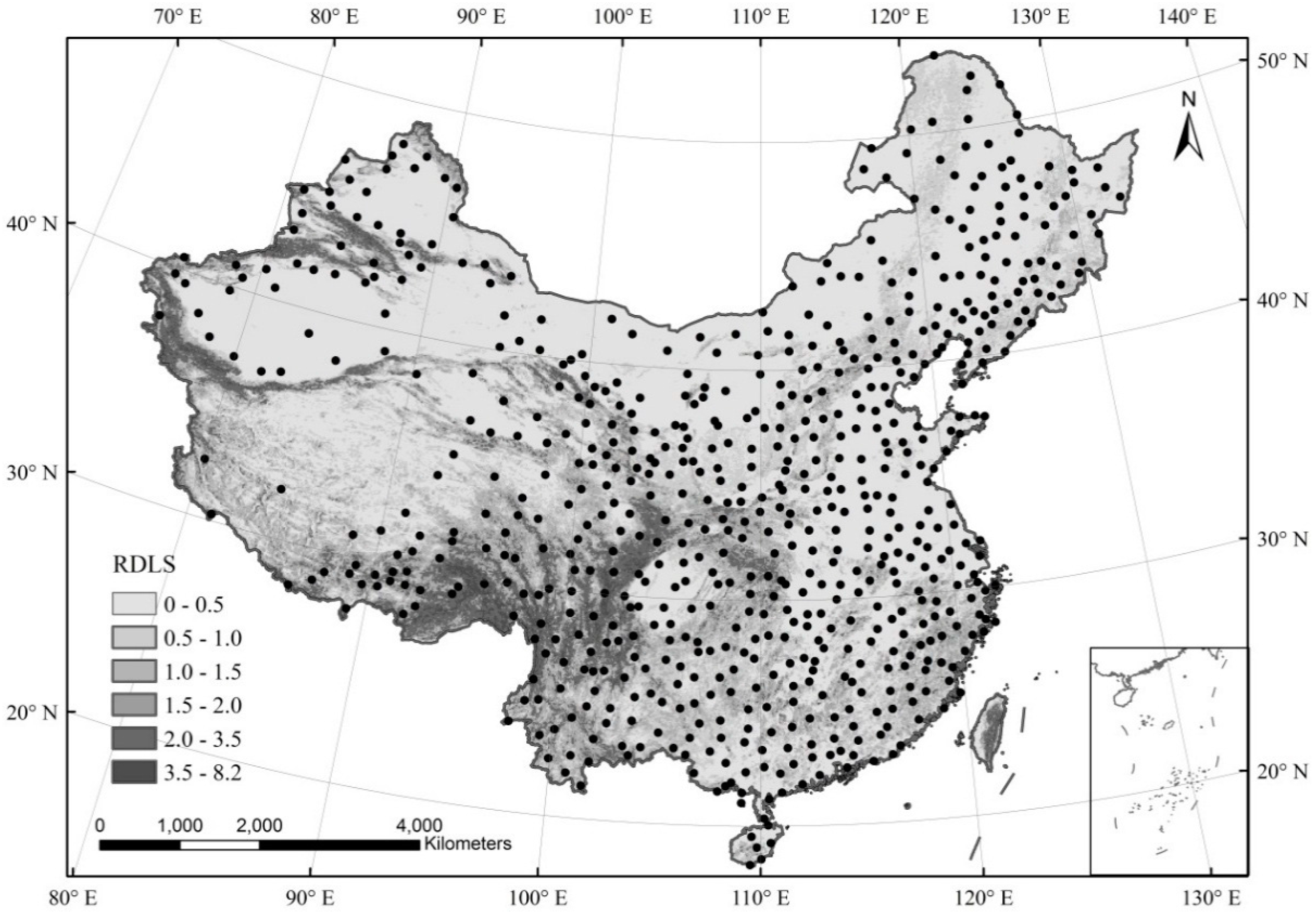
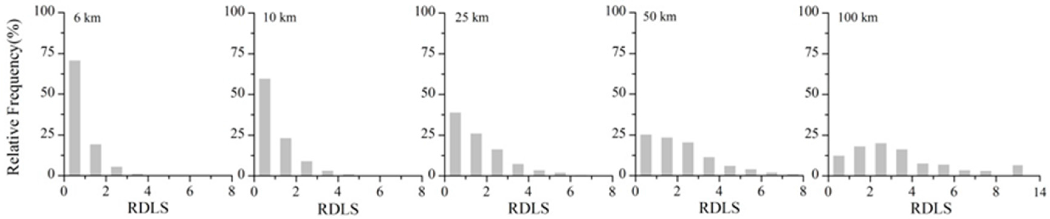
2.3. Relief Degree of the Land Surface

Due to the influence of topographic relief, mountain temperature variability is more complicated because mountainous terrain experiences a broader range of spatiotemporal scales than flat terrain [34,48,49]. The inhomogeneous surface heat flux modulates the turbulence structure, and there are strong lateral heat fluxes due to topography variability, violating the generally assumption of predominantly vertical heat transport [37,50]. However, on relatively flat terrain and vegetation, the horizontal homogeneity leads to stable atmospheric conditions [51]. In mountainous regions, the topography determines the temperature through the variations in solar radiation loading on different slope orientations [36,37,38]. Furthermore, Ta is affected more by the wind and free-air advection from mountains than the local sensible heat fluxes [52,53,54].
To characterize the effects of the topography on the surface thermal processes, we derived a topographic index (the relief degree of the land surface, RDLS) from the elevation [55]:
RDLS = Max ( H ) i Min ( H ) i 1 P ( A ) i / A i / 500 ,
where Max(H) is the maximum grid-cell elevation, Min(H) is the minimum grid-cell elevation, and P(A) is the flat plain area, A is the total area, i is the spatial window, and 500 is the benchmark mountain height in China. The RDLS value reflects the level of terrain relief relative to the surrounding environment. A value less than one indicates that the relative elevation difference does not exceed 500 m, while a value greater than one indicates a difference of more than 500 m. The elevation data were obtained from the weather stations.
To further characterize the influence of topography on the ground thermal regime, we developed a multi-scale topography index (RDLS) based on elevation. The RDLS for a specific window size reflects the altitudinal gradient of a grid cell relative to the surrounding terrain. We calculated the multi-scale RDLS across five spatial window sizes, including 6, 10, 25, 50, and 100 km. Generally, the RDLS value was concentrated in the range of 0 to 1, indicating that most of the altitude difference across China is less than 500 m. However, the value of the RDLS appeared to increase as the spatial window size increased, and its distribution became homogeneous.
As illustrated in Figure 1 and Figure 2, the RDLS calculated using spatial window sizes less than 25 km that were capable of capturing distinct terrain patterns across China. The percentages of RDLS within the range of 0 to 1 were 71.5% and 60.3% for the 6 km and 10 km spatial resolutions, respectively, whereas the RDLS at spatial resolutions larger than 25 km were too coarse to fully describe the terrain relief between the plain and mountainous areas. The percentage of RDLS in different groups gradually decreased as the spatial resolution decreased. The percentage of the RDLS that was within the range of 0 to 1 decreased from 39.7% at the 25 km resolution to 13.1% at the 100 km resolution, and the percentage tended to distribute evenly across the entire range. Because the spatial window size has a serious impact on the RDLS value, the selection of window size should objectively account for the spatial terrain variation. The RDLS threshold to distinguish terrain relief also varied with the spatial window sizes. Therefore, the RDLS in the present study that was calculated at 6 km resolution is capable of capturing the distinctive terrain features and being in accordance with the resolution of the remotely sensed data.

3. Results

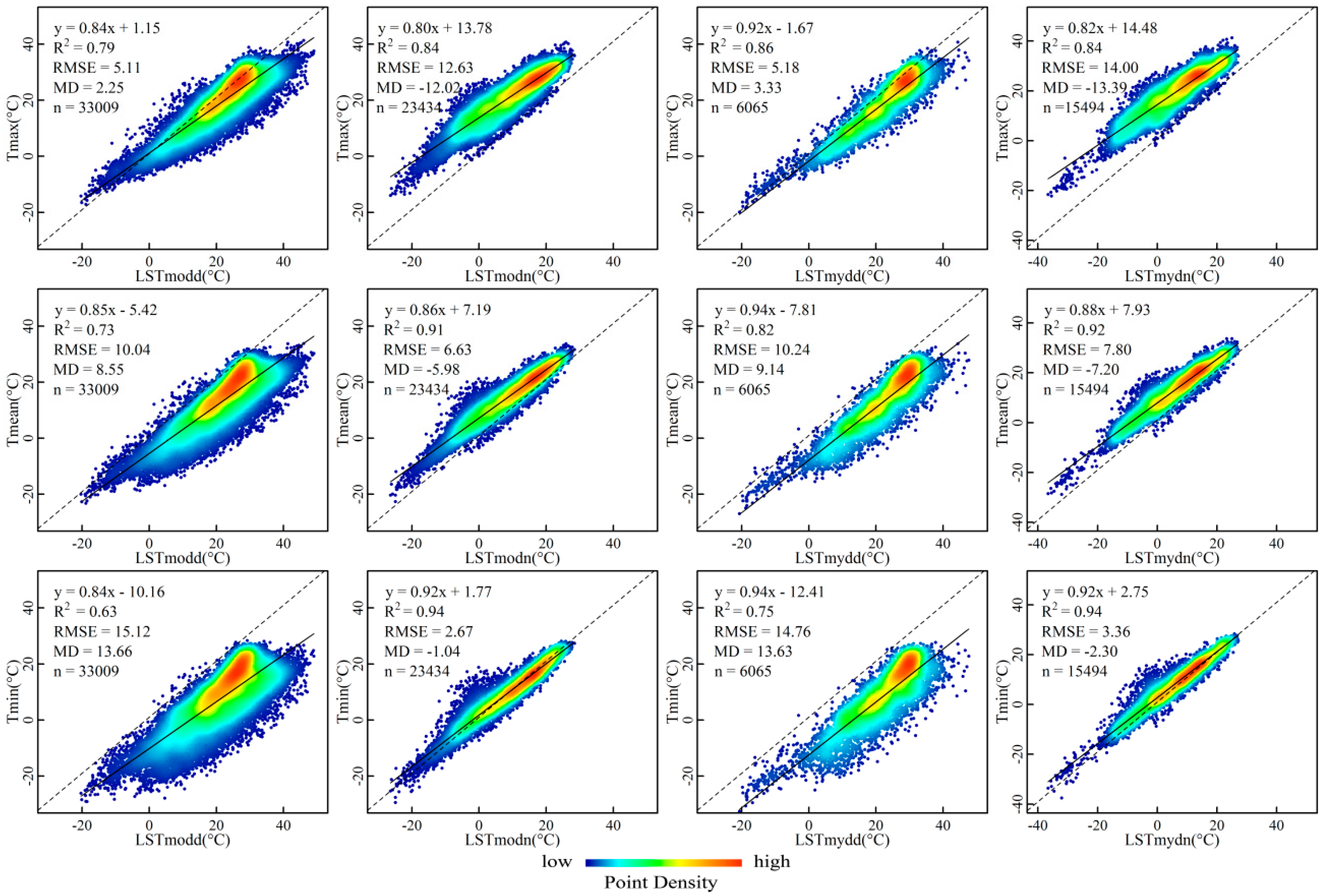
3.1. Relationships between the Ta and the Four LST Products over China

Both the Terra and Aqua LST products were compared with the ground-based monthly Ta to determine the optimum predictor for simulating Ta. As shown in the point density plots (Figure 3), the nighttime LST datasets (LSTmodn and LSTmydn) and the observed Ta are more linearly concentrated along the fitting line than the daytime datasets. Strong correlations were observed between the nighttime LST and Tmean and Tmin with minimal bias (R2 > 0.90, RMSE and mean difference (MD) < 7 °C). Specifically, the LSTmodn tends to be more accurate for the estimation of Ta with lower intercepts, smaller biases and larger sample sizes than LSTmydn. For Tmax, the LSTmydd had good agreement with a slope of –1 and an intercept of less than 2 °C. This is most likely due to the fact that the Aqua overpass time (1:30 pm) is closest to the time when Tmax was recorded. However, the LSTmydd was inapplicable for retrieving Ta due to the data scarcity. As a consequence, LSTmodn seems to be best for linear estimation of Tmax, Tmean and Tmin among the LST products.

3.2. Model Building

As expected, good agreement between LSTmodn and the observed Ta (2000–2005) is observed in China (R2 > 0.8, slope–1) (Figure 4). The RMSE ranges from 2.6 °C to 12.6 °C, and the MD varies from −12.0 °C to −1.1 °C. The LSTmodn tends to match Tmin best (R2, slope and MD–1) but shows large biases toward Tmax and Tmean. This is most likely due to the LSTmodn overpass time (10:30 pm), which is closer to the time when Tmin was recorded than when Tmax and Tmean were recorded, thus reducing the difference. However, some of the comparison scatter points are more scattered above the regression line. As indicated by the red circle in Figure 4, the linear LSTmodn-Ta relationship is significantly attenuated by this outlier dataset, revealing a triangular trend. The surface thermal dynamics are strongly influenced by the local surface features. Consequently, we identify this outlier dataset as collected from the Himalayas and the Hengduan mountain area located in southwest China where the elevation exceeds 1000 m (digital elevation model (DEM) > 1000 m) and the topographic relief is more than 600 m (RDLS > 1.2) (Figure 1). The complicated LSTmodn-Ta relationship in the Himalayas and the Hengduan mountain area is modified by the complex terrain and its related factors, such as elevation and solar radiation interception.
Based on the findings, we attempted to divide the comparison datasets into two parts, i.e., linear and nonlinear datasets, according to the altitudinal gradient. The former dataset exhibits a stable and simple linear relationship (0.86 ≤ R2 ≤ 0.95) between LSTmodn and Ta in the flat terrain areas (DEM ≤ 1000 m and RDLS ≤ 1.2); therefore, this dataset could be treated as empirical and used in applications. However, the latter dataset tends to show a triangular trend because it covers mountainous areas with relatively large local topographic reliefs (DEM > 1000 m and RDLS > 1.2). The nonlinear comparison dataset showed that the LSTmodn dramatically underestimated Tmax (MD = −17.8 °C, slope = 0.68), resulting in the largest estimated bias (RMSE = 17.5 °C), followed by Tmean (RMSE = 10.4 °C, MD = −9.7 °C) and Tmin (RMSE = 5.9 °C, MD = −4.2 °C). Because the simple linear relationship is unable to fully clarify the LSTmodn-Ta relationship in the high altitude variation mountainous regions, the additional terrain-related variables should be incorporated to consider the effects of complex terrain on surface heat flux. A multiple linear regression model was built to select relevant environmental parameters into the LSTmodn-Ta relationship through stepwise regression analysis. The NDVI and LST are partially correlated with season [27,56,57], so the NDVI variable is incorporated only during the growing season from May to October. The simple and multiple linear regression models corresponding to different regions and seasons are shown in Table 1.

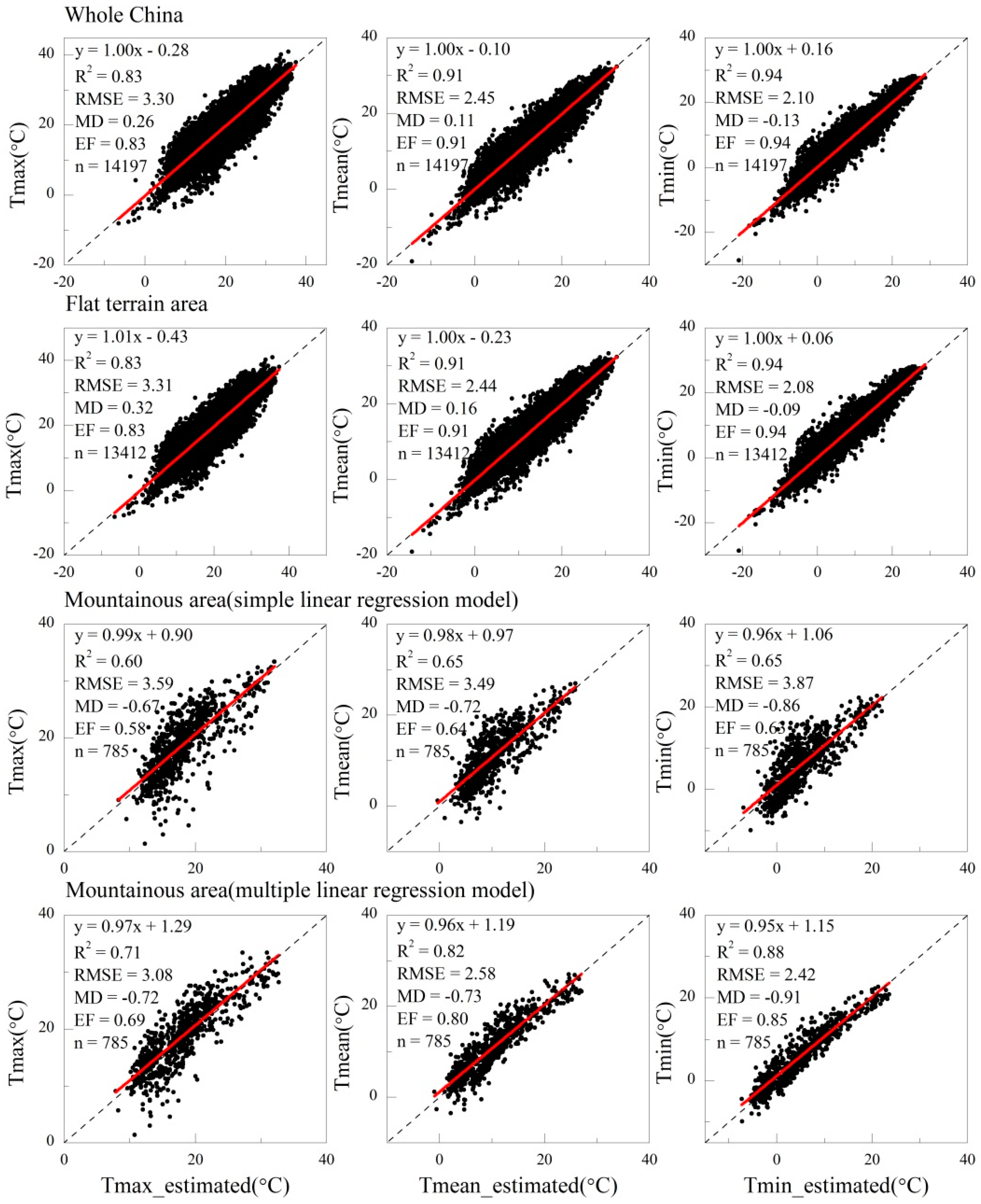
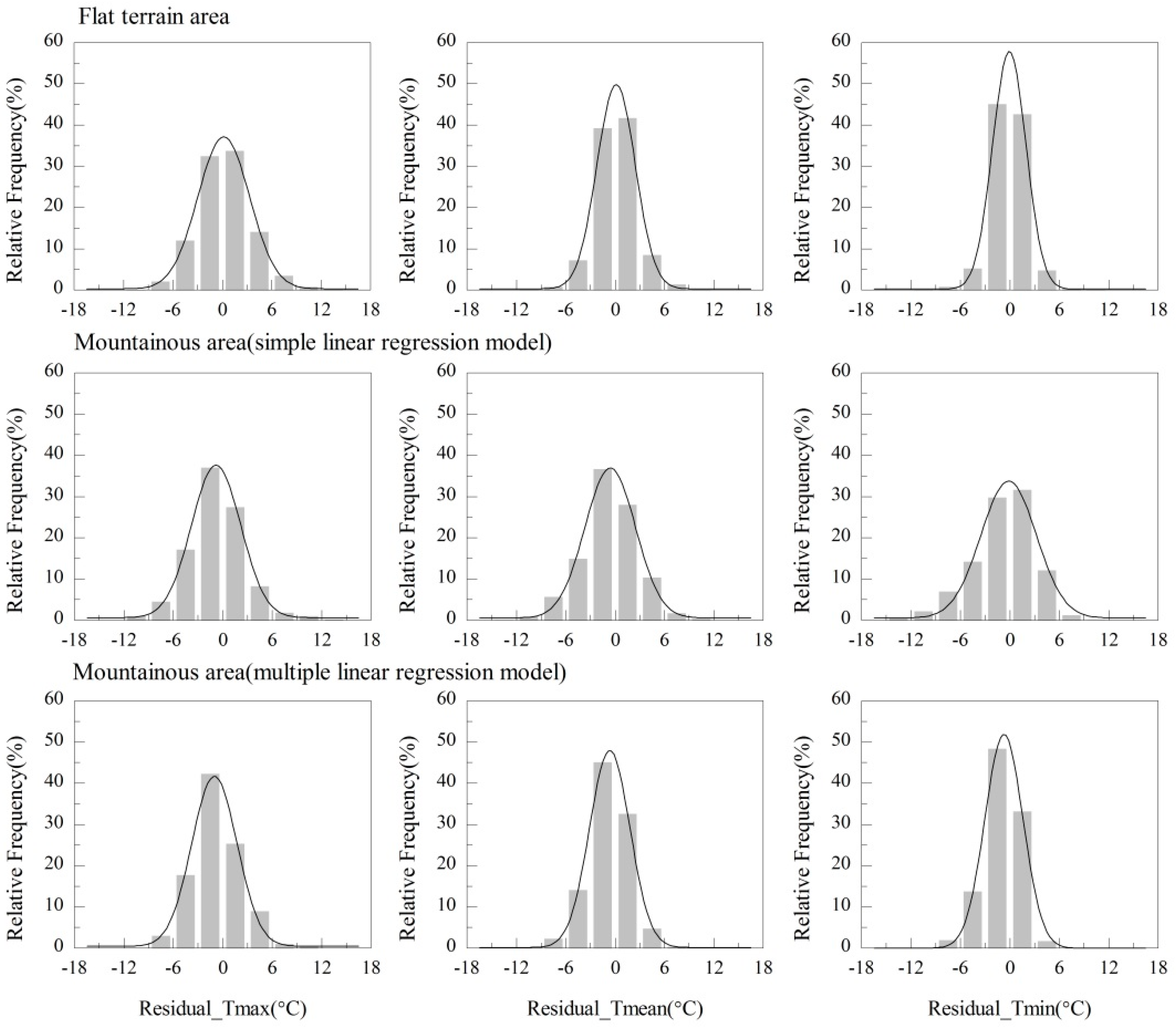
3.3. Model Validation

To assess the model performance, the Ta from routine meteorological stations (2006–2010) is used as the reference to validate the estimated Ta (Figure 5). The simple and multiple linear regression models exhibit good performance in the estimation of Ta in flat terrain and mountainous areas, respectively. The multiple linear regression model including NDVI, elevation, and AH can effectively interpret the LSTmodn–Ta relationship in the heterogeneous landscape of China. The Ta that are predicted over the entirety of China by combining the flat terrain area and mountainous area (multiple linear regression model) fit well with the observed Ta, yielding MD and intercepts close to 0 °C, as well as slopes and model efficiencies (EF) close to 1. Furthermore, the accuracy of the estimated Tmax and Tmean were significantly improved with the fitting line close to the 1:1 line.
In the flat terrain area, the monthly Ta is estimated as a function of LSTmodn and is highly consistent with the observed Ta. The frequency distribution of the estimation residual is symmetrical around zero (Figure 6). The relative frequency of the residual is largely concentrated within the range −3 °C and 3 °C (66%–88%). The average observed Tmax, Tmean, and Tmin are 21.2 °C (ranging from −8.1 °C to 41.0 °C), 15.4 °C (ranging from −19.1 °C to 33.3 °C), and 10.8 °C (ranging from −28.6 °C to 28.1 °C), respectively. The average simulated Tmax, Tmean, and Tmin are 21.5 °C (ranging from −6.5 °C to 37.4 °C), 15.6 °C (ranging from −14.3 °C to 32.5 °C), and 10.7 °C (ranging from −21.0 °C to 28.7 °C), respectively, showing a perfect match with the observed Ta. However, in the southwest mountainous area, the multiple linear regression model is developed to derive Ta, and the outcomes are encouraging. As shown in Figure 5, the monthly Ta predicted by the multiple linear regression model appears to be more linearly correlated with the observed Ta than the simple linear regression model. By applying the multiple linear regression model, the correlation coefficient of R2 increased substantially from 0.60–0.65 to 0.71–0.88. Meanwhile, the RMSE decreased from 3.49–3.87 to 2.42–3.08, and the distribution of the estimation residual is more concentrated around 0 °C (Figure 6). Furthermore, the EF values of the multiple linear regression models are closer to 1, indicating a better description of the observed mean than that of the simple linear regression model.

4. Discussion

4.1. The Accuracy of the Daytime and Nighttime LST for Ta Estimation

Terra nighttime LST shows the best agreement with the observed Ta in China (with the exception of Tmax), and the RMSE validation errors are 6.6 °C and 2.7 °C for Tmean and Tmin, respectively (Figure 3). The fact that the MODIS nighttime LST products result in better predicted Ta accuracies is also verified by the work of [14,53]. During the nighttime, due to the radiative cooling at the surface, the air will generally be stably stratified and thus the turbulence generated by surface friction will be weakened [58,59]. The earth surface behaves almost as an isothermal and homogeneous surface, simplifying the retrieval process and improving the estimation accuracy of the air temperature [24,60,61]. However, in the daytime, the influences of direct solar illumination, the surface and weather conditions and the satellite itself result in more complex interactions between Ta and LST [17,24]. The solar radiation is first absorbed by the ground, which then heats the near surface air. As the temperature increases and more thermal energy is concentrated at the surface, the daytime LST and Ta become increasingly decoupled [62], which is why the daytime LST is hotter than the observed Ta and their points are more scattered around the 1:1 line (Figure 3). In addition, a much larger effect from angular anisotropy on the remote sensing data products is expected for daytime LST than for nighttime LST due to the sunlight and shade effects within pixels during the daytime [15,63].
However, Mildrexler et al. [62] indicated that the daytime LST from Aqua had a strong positive correlation with Tmax globally, and Shen and Leptoukh [16] precisely derived Tmax from the Terra daytime LST over central and eastern Eurasia as the mean absolute error (MAE) varied from 2.4 °C to 3.2 °C. The above studies also noted that their relationship greatly depended on the land cover type; a denser canopy resulted in more closely coupled daytime LST and Tmax. The Aqua/Terra LST overpass in the day is closer to the time when Tmax was recorded, which should be better at estimating Tmax than nighttime LST [14]. However, Zeng et al. [64] found that a stronger correlation existed between Tmax and nighttime LST than between Tmax and daytime LST in estimating daily Ta over the US corn belt. Zhu et al. [65] and Lin et al. [66] found that the difference between daytime LST and Tmax was still too large with MAE being 6.21 °C and 8.12 °C for LSTmodd and LSTmydd, respectively. Furthermore, Huang et al. [67] retrieved daily Ta in central China, which showed similar results to this study that the RMSE of LSTmydd (2.6–4.2 °C) was larger than LSTmodn (1.9–2.5 °C). As further interpreted by Fu et al. [22] and Mostovoy et al. [68], the time discrepancy between the moment of the satellite overpass and the time when Tmax or Tmin occurred was not a key factor controlling the relationship between Ta and LST.

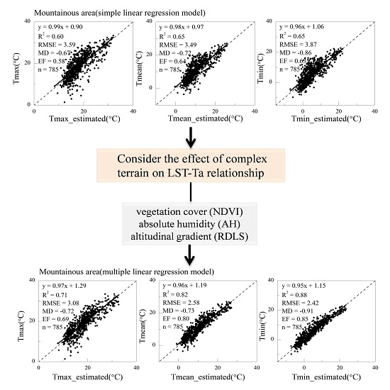
4.2. Using the Multiple Linear Regression Model to Derive Ta in Mountainous Areas

The LST and Ta are correlated due to the heat exchange between the surface and the atmosphere. This study found that combining the remote sensing LST and physiographic factors had the potential to improve the accuracy of estimating Ta in large regions. This finding was similar to the results of [12,69,70]. Combining the simple and multiple linear regression models exhibited a good performance in the estimation of Ta over the entirety of China, yielding RMSE ranging from 2.1 °C to 3.3 °C and MD from −0.13 °C to 0.26 °C (Figure 5). Zhang et al. [14] included the solar declination into the estimation of China daily Ta, resulting in a relatively large error where the MD were within 1.61 °C–3.32 °C and the RMSE from 2.08 °C to 4.10 °C. Yao et al. [71] retrieved monthly Tmean based on 72 weather stations in the southeastern Tibetan Plateau, yielding RMSE within 2.25 °C–3.23 °C, which showed the same accuracy as that in this study in mountainous areas (2.42 °C ≤ RMSE ≤ 3.08 °C). Zheng et al. [72] and Chen et al. [69] derived the monthly Ta over Northern China and the entirety of China, obtaining more accurate results with RMSE within 0.86 °C–1.13 °C and 0.80 °C–1.29 °C due to the combination of interpolation techniques.
The heat transfer process is strongly influenced by the local radiation budget and the atmospheric contribution [53,73]. In mountainous regions, Ta is affected more by the wind and free-air advection from mountains than the local sensible heat fluxes; thus, it agrees less with LST [53,54]. Additionally, in the high mountains, during snow-covered periods, the linear correlation between the air and ground surface temperatures becomes weaker than that in snow-free periods [74]. Many studies have highlighted the importance of the vegetation cover, topography and climate conditions on the estimation of Ta from LST over complex terrain [4,17,75]. To adequately interpret the relationship between LST and Ta, it is essential to take the local climate and surrounding environment into consideration. However, NDVI of alpine areas is unusable in the non-growing season because of snow and bare ground [24,76]. The assumption of linear and negative slopes between LST and NDVI is, therefore, not applicable. Including NDVI in the regression model did not significantly improve the estimation accuracy, with the estimated R2 improved trivially, from 0.73 to 0.76, 0.81 to 0.83, and 0.83 to 0.83 for Tmax, Tmean, and Tmin, respectively. By applying the multiple linear regression model in this study, the RMSE were 14%–37% smaller than those from the simple linear regression model (Figure 5). Correspondingly, the distribution of the estimation residual was more concentrated around 0 °C (Figure 6). Furthermore, the EF values and R2 of the multiple linear regression models were closer to 1, indicating a better description of the observed mean than that of the simple linear regression model.
The Himalayas and Hengduan mountains located in the southwest of China are generally covered with alpine vegetation during warm growing seasons, while they are covered with dry grass residuals or snow during non-growing seasons. The seasonal vegetation greening tends to increase the spatial heterogeneity of the LST [77]. Dry, bare, and low-density soil has relatively low thermal inertia, resulting in large temperature variations and high LSTs [78,79], while dense vegetation induces more transpiration and blocks incident shortwave radiation, efficiently preventing the surface temperature from increasing with the air temperature during the daytime, which cools the surface [27,36]. Meanwhile, the climate conditions on the Tibetan Plateau also play major roles in the land surface-atmosphere interactions. Tanaka et al. [80,81] found that the ground surface and surface atmosphere layer on the Tibetan Plateau were very dry until the monsoon progressed. In summer, the strong activity of the convection cloud and mesoscale convection systems on the southern Plateau at a latitude of 33° N, accompanied by the remarkable mountain uplift, resulted in heavy rainfall and high water vapor content in the mountain areas of southwest China [82,83]. This area is rather close to a relatively large local topographic relief area (DEM > 1000 m and RDLS > 1.2). In addition, the Tibetan Plateau warming in summer induces an upward transfer of sensible heat flux, which then destabilizes the atmosphere and promotes convection, leading to more precipitation [84]. This high atmospheric water content in the complex topography contributes to the large error in the LST determined from spectral emissivity [85,86].

5. Conclusions

In this study, we assessed the potential of MODIS LST for the estimation of monthly Ta through linear regression analysis of LST and observed the Ta from 688 meteorological stations in China. The Terra nighttime LST data (LSTmodn) was proven to be accurate enough for linear estimation of the monthly Tmean and Tmin with strong correlation (R2 > 0.90) and minimal bias (RMSE and MD < 7 °C) among the other LST products despite their overpass time discrepancies. Because the LSTmodn and Ta are well coupled in the flat terrain areas (DEM ≤ 1000 m and RDLS ≤ 1.2), the Ta can be accurately estimated as a function of LSTmodn, yielding MD less than 0.5 °C, model efficiencies (EF) close to 1, and RMSE ranging from 2.08 °C to 3.31 °C.
However, in the mountainous areas of southwest China, a complex topography leads to a complicated thermal mechanism. To clarify the complex LSTmodn-Ta relationship, the physiographic factors closely linked to energy processes were taken into account. This study develops a feasibility proxy to retrieve Ta that includes the influences of the seasonal vegetation cover (NDVI) and the ambient absolute humidity (AH) by stepwise regression analysis according to the different topographical reliefs. The multiple linear model can effectively improve the estimated accuracy by significantly increasing the R2 from 0.60–0.65 to 0.71–0.88 and decreasing the RMSE from 3.49 °C–3.87 °C to 2.42 °C–3.08 °C in the mountainous areas (DEM > 1000 m and RDLS > 1.2). This result suggested that a large terrain relief can significantly influence the spatial pattern of the climate and thus modify the surface energy flux. This finding becomes critically helpful in interpreting the LSTmodn-Ta relationship by considering the complicated hydrothermal circulation in complex terrain. Therefore, further studies should consider the local physiographic features contributing to the land surface-atmosphere interaction mechanism by reducing the bias of Ta determined from satellite LST.

Acknowledgments

This study was supported by the National Basic Research Program of China (973 Program, No. 2014CB954303) and the National Natural Science Foundation of China (Nos. 41321064, 41573069). We thank the National Meteorological Center, China Meteorological Administration, for providing observational meteorological data and the Land Processes Distributed Active Archive Center (LPDAAC) for providing MODIS images.

Author Contributions

Yao Huang and Wen Zhang conceived and designed the research. Xiaohui Lin and Wenjuan Sun performed the data analysis and model development. Pengfei Han, Lingfei Yu and Feifei Sun made the data processing. Xiaohui Lin and Wen Zhang wrote the manuscript with contribution from all the co-authors.

Conflicts of Interest

The authors declare no conflicts of interest.

References

  1. Wang, K.; Li, Z.; Cribb, M. Estimation of evaporative fraction from a combination of day and night land surface temperatures and ndvi: A new method to determine the priestley–taylor parameter. Remote Sens. Environ. 2006, 102, 293–305. [Google Scholar] [CrossRef]
  2. Norman, J.M.; Kustas, W.P.; Humes, K.S. Source approach for estimating soil and vegetation energy fluxes in observations of directional radiometric surface temperature. Agric. For. Meteorol. 1995, 77, 263–293. [Google Scholar] [CrossRef]
  3. Betts, A.K.; Ball, J.H.; Beljaars, A.; Miller, M.J.; Viterbo, P.A. The land surfa-ceatmosphere interaction: A review based on observational and global modeling perspectives. J. Geophys. Res. Atmos. 1996, 101. [Google Scholar] [CrossRef]
  4. Oyler, J.W.; Ballantyne, A.; Jencso, K.; Sweet, M.; Running, S.W. Creating a topoclimatic daily air temperature dataset for the conterminous united states using homogenized station data and remotely sensed land skin temperature. Int. J. Climatol. 2015, 35, 2258–2279. [Google Scholar] [CrossRef]
  5. Harris, I.; Jones, P.; Osborn, T.; Lister, D. Updated high-resolution grids of monthly climatic observations-the cru ts3. 10 dataset. Int. J. Climatol. 2014, 34, 623–642. [Google Scholar] [CrossRef] [Green Version]
  6. Stocker, T.; Qin, D.; Plattner, G.; Tignor, M.; Allen, S.; Boschung, J.; Nauels, A.; Xia, Y.; Bex, B.; Midgley, B. IPCC, 2013: Climate Change 2013: The Physical Science Basis. Contribution of Working Group I to the fifth Assessment Report of the Intergovernmental Panel on Climate Change; Cambridge University Press: Cambridge, UK; New York, NY, USA, 2013. [Google Scholar] [CrossRef]
  7. Kalnay, E.; Kanamitsu, M.; Kistler, R.; Collins, W.; Deaven, D.; Gandin, L.; Iredell, M.; Saha, S.; White, G.; Woollen, J. The ncep/ncar 40-year reanalysis project. Bull. Am. Meteorol. Soc. 1996, 77, 437–471. [Google Scholar] [CrossRef]
  8. Uppala, S.M.; Kållberg, P.; Simmons, A.; Andrae, U.; Bechtold, V.D.; Fiorino, M.; Gibson, J.; Haseler, J.; Hernandez, A.; Kelly, G. The era-40 re-analysis. Q. J. R. Meteorol. Soc. 2005, 131, 2961–3012. [Google Scholar] [CrossRef]
  9. Stahl, K.; Moore, R.; Floyer, J.; Asplin, M.; McKendry, I. Comparison of approaches for spatial interpolation of daily air temperature in a large region with complex topography and highly variable station density. Agric. For. Meteorol. 2006, 139, 224–236. [Google Scholar] [CrossRef]
  10. Holden, Z.A.; Abatzoglou, J.T.; Luce, C.H.; Baggett, L.S. Empirical downscaling of daily minimum air temperature at very fine resolutions in complex terrain. Agric. For. Meteorol. 2011, 151, 1066–1073. [Google Scholar] [CrossRef]
  11. Stisen, S.; Sandholt, I.; Nørgaard, A.; Fensholt, R.; Eklundh, L. Estimation of diurnal air temperature using msg seviri data in west Africa. Remote Sens. Environ. 2007, 110, 262–274. [Google Scholar] [CrossRef]
  12. Benali, A.; Carvalho, A.; Nunes, J.; Carvalhais, N.; Santos, A. Estimating air surface temperature in portugal using modis lst data. Remote Sens. Environ. 2012, 124, 108–121. [Google Scholar] [CrossRef]
  13. Cristóbal, J.; Ninyerola, M.; Pons, X. Modeling air temperature through a combination of remote sensing and gis data. J. Geophys. Res. Atmos. 2008, 113. [Google Scholar] [CrossRef]
  14. Zhang, W.; Huang, Y.; Yu, Y.; Sun, W. Empirical models for estimating daily maximum, minimum and mean air temperatures with modis land surface temperatures. Int. J. Remote. Sens. 2011, 32, 9415–9440. [Google Scholar] [CrossRef]
  15. Zheng, X.; Zhu, J.; Yan, Q. Monthly air temperatures over northern China estimated by integrating modis data with gis techniques. J. Appl. Meteorol. Clim. 2013, 52, 1987–2000. [Google Scholar] [CrossRef]
  16. Shen, S.; Leptoukh, G.G. Estimation of surface air temperature over central and eastern eurasia from modis land surface temperature. Environ. Res. Lett. 2011, 6. [Google Scholar] [CrossRef]
  17. Kloog, I.; Chudnovsky, A.; Koutrakis, P.; Schwartz, J. Temporal and spatial assessments of minimum air temperature using satellite surface temperature measurements in massachusetts, USA. Sci. Total. Environ. 2012, 432, 85–92. [Google Scholar] [CrossRef] [PubMed]
  18. Wan, Z. New refinements and validation of the modis land-surface temperature/emissivity products. Remote Sens. Environ. 2008, 112, 59–74. [Google Scholar] [CrossRef]
  19. Liu, D.; Pu, R. Downscaling thermal infrared radiance for subpixel land surface temperature retrieval. Sensors 2008, 8, 2695–2706. [Google Scholar] [CrossRef]
  20. Jin, M.; Dickinson, R.E. Land surface skin temperature climatology: Benefitting from the strengths of satellite observations. Environ. Res. Lett. 2010, 5. [Google Scholar] [CrossRef]
  21. Shreve, C. Working towards a community-wide understanding of satellite skin temperature observations. Environ. Res. Lett. 2010, 5. [Google Scholar] [CrossRef]
  22. Fu, G.; Shen, Z.; Zhang, X.; Shi, P.; Zhang, Y.; Wu, J. Estimating air temperature of an alpine meadow on the northern tibetan plateau using modis land surface temperature. Acta Ecol. Sin. 2011, 31, 8–13. [Google Scholar] [CrossRef]
  23. Prince, S.D.; Goetz, S.J.; Dubayah, R.; Czajkowski, K.; Thawley, M. Inference of surface and air temperature, atmospheric precipitable water and vapor pressure deficit using advanced very high-resolution radiometer satellite observations: Comparison with field observations. J. Hydrol. 1998, 212, 230–249. [Google Scholar] [CrossRef]
  24. Vancutsem, C.; Ceccato, P.; Dinku, T.; Connor, S.J. Evaluation of modis land surface temperature data to estimate air temperature in different ecosystems over africa. Remote Sens. Environ. 2010, 114, 449–465. [Google Scholar] [CrossRef]
  25. Recondo, C.; Peón, J.J.; Zapico, E.; Pendás, E. Empirical models for estimating daily surface water vapour pressure, air temperature, and humidity using modis and spatiotemporal variables. Applications to peninsular spain. Int. J. Remote. Sens. 2013, 34, 8051–8080. [Google Scholar] [CrossRef]
  26. Zhang, J.; Gao, S.; Chen, H.; Yu, J.; Tang, Q. Retrieval of the land surface-air temperature difference from high spatial resolution satellite observations over complex surfaces in the Tibetan Plateau. J. Geophys. Res. Atmos. 2015, 120. [Google Scholar] [CrossRef]
  27. Sun, D.; Kafatos, M. Note on the ndvi-lst relationship and the use of temperature-related drought indices over north america. Geophys. Res. Lett. 2007, 34. [Google Scholar] [CrossRef]
  28. Nieto, H.; Sandholt, I.; Aguado, I.; Chuvieco, E.; Stisen, S. Air temperature estimation with msg-seviri data: Calibration and validation of the tvx algorithm for the iberian peninsula. Remote Sens. Environ. 2011, 115, 107–116. [Google Scholar] [CrossRef]
  29. Shukla, J.; Mintz, Y. Influence of land-surface evapotranspiration on the earth's climate. Science 1982, 215, 1498–1501. [Google Scholar] [CrossRef] [PubMed]
  30. Coll, C.; Caselles, V.; Galve, J.M.; Valor, E.; Niclos, R.; Sánchez, J.M.; Rivas, R. Ground measurements for the validation of land surface temperatures derived from aatsr and modis data. Remote Sens. Environ. 2005, 97, 288–300. [Google Scholar] [CrossRef]
  31. Jiménez-Muñoz, J.C.; Sobrino, J.A. A generalized single-channel method for retrieving land surface temperature from remote sensing data. J. Geophys. Res. Atmos. 2003, 108. [Google Scholar] [CrossRef]
  32. Maeda, E.E. Downscaling modis lst in the east african mountains using elevation gradient and land-cover information. Int. J. Remote. Sens. 2014, 35, 3094–3108. [Google Scholar] [CrossRef]
  33. Stroppiana, D.; Antoninetti, M.; Brivio, P.A. Seasonality of modis lst over southern italy and correlation with land cover, topography and solar radiation. Eur. J. Remote Sens. 2014, 47, 133–152. [Google Scholar] [CrossRef]
  34. Lundquist, J.D.; Cayan, D.R. Surface temperature patterns in complex terrain: Daily variations and long-term change in the central sierra nevada, california. J. Geophys. Res. Atmos. 2007, 112. [Google Scholar] [CrossRef]
  35. Yang, H.; Liua, Y.; Yang, Y.; Zhang, C. Estimation and Analysis of Land Surface Water and Heat Fluxes in Mountain-Plain Area Based on Remote Sensing and Dem. In Proceedings of the 2009 17th International Conference on Geoinformatics, Fairfax, VA, USA, 12–14 August 2009.
  36. Van De Kerchove, R.; Lhermitte, S.; Veraverbeke, S.; Goossens, R. Spatio-temporal variability in remotely sensed land surface temperature, and its relationship with physiographic variables in the russian altay mountains. Int. J. Appl. Earth Obs. 2013, 20, 4–19. [Google Scholar] [CrossRef] [Green Version]
  37. Noetzli, J.; Gruber, S.; Kohl, T.; Salzmann, N.; Haeberli, W. Three-dimensional distribution and evolution of permafrost temperatures in idealized high-mountain topography. J. Geophys. Res. Earth Surf. 2007, 112. [Google Scholar] [CrossRef] [Green Version]
  38. Mittaz, C.; Hoelzle, M.; Haeberli, W. First results and interpretation of energy-flux measurements over alpine permafrost. Ann. Glaciol. 2000, 31, 275–280. [Google Scholar] [CrossRef]
  39. Bertoldi, G.; Notarnicola, C.; Leitinger, G.; Endrizzi, S.; Zebisch, M.; Della Chiesa, S.; Tappeiner, U. Topographical and ecohydrological controls on land surface temperature in an alpine catchment. Ecohydrology 2010, 3, 189–204. [Google Scholar] [CrossRef]
  40. Yang, Y.; Mohammat, A.; Feng, J.; Zhou, R.; Fang, J. Storage, patterns and environmental controls of soil organic carbon in China. Biogeochemistry 2007, 84, 131–141. [Google Scholar] [CrossRef]
  41. Jiang, Y. Estimation of monthly mean daily diffuse radiation in china. Appl. Energ. 2009, 86, 1458–1464. [Google Scholar] [CrossRef]
  42. Snyder, R.L.; Melo-Abreu, J.P. Frost Protection: Fundamentals, Practice and Economics. Volume 1; Environment and Natural Resources Service Series; FAO: Rome, Italy, 2005; pp. 219–221. [Google Scholar]
  43. Reber, E.E.; Swope, J.R. On the correlation of the total precipitable water in a vertical column and absolute humidity at the surface. J. Appl. Meteorol. 1972, 11, 1322–1325. [Google Scholar] [CrossRef]
  44. Moderate Resolution Imaging Spectroradiometer (Modis). Available online: Https://ladsweb.Nascom.Nasa.Gov/data/ (accessed on 6 September 2015).
  45. Wan, Z.; Dozier, J. A generalized split-window algorithm for retrieving land-surface temperature from space. IEEE Trans. Geosci. Remote Sens. 1996, 34, 892–905. [Google Scholar]
  46. Crosson, W.L.; Al-Hamdan, M.Z.; Hemmings, S.N.; Wade, G.M. A daily merged modis aqua–terra land surface temperature data set for the conterminous united states. Remote Sens. Environ. 2012, 119, 315–324. [Google Scholar] [CrossRef]
  47. Ryu, Y.; Kang, S.; Moon, S.-K.; Kim, J. Evaluation of land surface radiation balance derived from moderate resolution imaging spectroradiometer (modis) over complex terrain and heterogeneous landscape on clear sky days. Agric. For. Meteorol. 2008, 148, 1538–1552. [Google Scholar] [CrossRef]
  48. Blandford, T.R.; Humes, K.S.; Harshburger, B.J.; Moore, B.C.; Walden, V.P.; Ye, H. Seasonal and synoptic variations in near-surface air temperature lapse rates in a mountainous basin. J. Appl. Meteorol. Clim. 2008, 47, 249–261. [Google Scholar] [CrossRef]
  49. Rolland, C. Spatial and seasonal variations of air temperature lapse rates in alpine regions. J. Clim. 2003, 16, 1032–1046. [Google Scholar] [CrossRef]
  50. Shen, S.; Leclerc, M.Y. How large must surface inhomogeneities be before they influence the convective boundary layer structure? A case study. Q. J. R. Meteorol. Soc. 1995, 121, 1209–1228. [Google Scholar] [CrossRef]
  51. Baldocchi, D.; Falge, E.; Gu, L.; Olson, R. Fluxnet: A new tool to study the temporal and spatial variability of ecosystem-scale carbon dioxide, water vapor, and energy flux densities. Bull. Am. Meteorol. Soc. 2001, 82, 2415–2434. [Google Scholar] [CrossRef]
  52. Pepin, N.; Lundquist, J. Temperature trends at high elevations: Patterns across the globe. Geophys. Res. Lett. 2008, 35. [Google Scholar] [CrossRef]
  53. Sohrabinia, M.; Zawar-Reza, P.; Rack, W. Spatio-temporal analysis of the relationship between lst from modis and air temperature in New Zealand. Theor. Appl. Climatol. 2014, 119, 567–583. [Google Scholar] [CrossRef]
  54. Hughes, M.; Hall, A.; Fovell, R.G. Dynamical controls on the diurnal cycle of temperature in complex topography. Clim. Dyn. 2007, 29, 277–292. [Google Scholar] [CrossRef]
  55. Feng, Z.; Tang, Y.; Yang, Y.; Zhang, D. The relief degree of land surface in china and its correlation with population distribution. Acta Geol. Sin. 2007, 62, 1073–1082. (in Chinese) . [Google Scholar]
  56. Julien, Y.; Sobrino, J.A.; Verhoef, W. Changes in land surface temperatures and ndvi values over europe between 1982 and 1999. Remote Sens. Environ. 2006, 103, 43–55. [Google Scholar] [CrossRef]
  57. Julien, Y.; Sobrino, J.A. The yearly land cover dynamics (ylcd) method: An analysis of global vegetation from ndvi and lst parameters. Remote Sens. Environ. 2009, 113, 329–334. [Google Scholar] [CrossRef]
  58. Holtslag, A.; De Bruin, H. Applied modeling of the nighttime surface energy balance over land. J. Appl. Meteorol. 1988, 27, 689–704. [Google Scholar] [CrossRef]
  59. Shamir, E.; Georgakakos, K.P. Modis land surface temperature as an index of surface air temperature for operational snowpack estimation. Remote Sens. Environ. 2014, 152, 83–98. [Google Scholar] [CrossRef]
  60. Wang, W.; Liang, S.; Meyers, T. Validating modis land surface temperature products using long-term nighttime ground measurements. Remote Sens. Environ. 2008, 112, 623–635. [Google Scholar] [CrossRef]
  61. Kestens, Y.; Brand, A.; Fournier, M.; Goudreau, S.; Kosatsky, T.; Maloley, M.; Smargiassi, A. Modelling the variation of land surface temperature as determinant of risk of heat-related health events. Int. J. Health Geogr. 2011, 10, 1–9. [Google Scholar] [CrossRef] [PubMed]
  62. Mildrexler, D.J.; Zhao, M.; Running, S.W. A global comparison between station air temperatures and modis land surface temperatures reveals the cooling role of forests. J. Geophys. Res. 2011, 116. [Google Scholar] [CrossRef]
  63. Pinheiro, A.C.; Privette, J.L.; Mahoney, R.; Tucker, C.J. Directional effects in a daily avhrr land surface temperature dataset over Africa. IEEE. Trans. Geosci. Remote Sens. 2004, 42, 1941–1954. [Google Scholar] [CrossRef]
  64. Zeng, L.; Wardlow, B.D.; Tadesse, T.; Shan, J.; Hayes, M.J.; Li, D.; Xiang, D. Estimation of daily air temperature based on modis land surface temperature products over the corn belt in the us. Remote Sens. 2015, 7, 951–970. [Google Scholar] [CrossRef]
  65. Zhu, W.; Lű, A.; Jia, S. Estimation of daily maximum and minimum air temperature using modis land surface temperature products. Remote Sens. Environ. 2013, 130, 62–73. [Google Scholar] [CrossRef]
  66. Lin, S.; Moore, N.J.; Messina, J.P.; DeVisser, M.H.; Wu, J. Evaluation of estimating daily maximum and minimum air temperature with modis data in east africa. Int. J. Appl. Earth Obs. 2012, 18, 128–140. [Google Scholar] [CrossRef]
  67. Huang, R.; Zhang, C.; Huang, J.; Zhu, D.; Wang, L.; Liu, J. Mapping of daily mean air temperature in agricultural regions using daytime and nighttime land surface temperatures derived from terra and aqua modis data. Remote Sens. 2015, 7, 8728–8756. [Google Scholar] [CrossRef]
  68. Mostovoy, G.V.; King, R.L.; Reddy, K.R.; Kakani, V.G.; Filippova, M.G. Statistical estimation of daily maximum and minimum air temperatures from modis lst data over the state of mississippi. Gisci. Remote Sens. 2006, 43, 78–110. [Google Scholar] [CrossRef]
  69. Chen, F.; Liu, Y.; Liu, Q.; Qin, F. A statistical method based on remote sensing for the estimation of air temperature in china. Int. J. Climatol. 2015, 35, 2131–2143. [Google Scholar] [CrossRef]
  70. Xu, Y.; Qin, Z.; Shen, Y. Study on the estimation of near-surface air temperature from modis data by statistical methods. Int. J. Remote. Sens. 2012, 33, 7629–7643. [Google Scholar] [CrossRef]
  71. Yao, Y.; Zhang, B. Modis-based air temperature estimation in the southeastern tibetan plateau and neighboring areas. J. Geogr. Sci. 2012, 22, 152–166. [Google Scholar] [CrossRef]
  72. Li, D.; Zhong, H.; Wu, Q.; zhang, Y.; Hou, Y.; Tang, M. Analyses on changes of surface temperature over qinghai-xizang plateau. Plateau Meteorol. 2005, 24, 291–298. [Google Scholar]
  73. Norman, J.M.; Becker, F. Terminology in thermal infrared remote sensing of natural surfaces. Agric. For. Meteorol. 1995, 77, 153–166. [Google Scholar] [CrossRef]
  74. Zhang, T. Influence of the seasonal snow cover on the ground thermal regime: An overview. Rev. Geophys. 2005, 43, RG4002. [Google Scholar] [CrossRef]
  75. Lai, Y.; Li, C.; Lin, P.; Wey, T.; Chang, C. Comparison of modis land surface temperature and ground-based observed air temperature in complex topography. Int. J. Remote. Sens. 2012, 33, 7685–7702. [Google Scholar] [CrossRef]
  76. Colombi, A.; De Michele, C.; Pepe, M.; Rampini, A. Estimation of daily mean air temperature from modis lst in alpine areas. EARSeL eProc. 2007, 6, 38–46. [Google Scholar]
  77. Xiang, T.; Vivoni, E.R.; Gochis, D.J. Seasonal evolution of ecohydrological controls on land surface temperature over complex terrain. Water Resour. Res. 2014, 50, 3852–3874. [Google Scholar] [CrossRef]
  78. Weng, Q.; Lu, D.; Schubring, J. Estimation of land surface temperature–vegetation abundance relationship for urban heat island studies. Remote Sens. Environ. 2004, 89, 467–483. [Google Scholar] [CrossRef]
  79. Weng, Q. Thermal infrared remote sensing for urban climate and environmental studies: Methods, applications, and trends. Isprs J. Photogramm. 2009, 64, 335–344. [Google Scholar] [CrossRef]
  80. Tanaka, K.; Ishikawa, H.; Hayashi, T.; Tamagawa, I.; Ma, Y. Surface energy budget at amdo on the tibetan plateau using game/tibet iop98 data. J. Meteorol. Soc. Jpn. 2001, 79, 505–517. [Google Scholar] [CrossRef]
  81. Tanaka, K.; Tamagawa, I.; Ishikawa, H.; Ma, Y.; Hu, Z. Surface energy budget and closure of the eastern tibetan plateau during the game-tibet iop 1998. J. Hydrol. 2003, 283, 169–183. [Google Scholar] [CrossRef]
  82. Jixi, J.; Meizhu, F. Convective clouds and mesoscale convective systems over the tibetan plateau in summer. Chin. J. Atmos. Sci. 2002, 26, 263–270. (in Chinese). [Google Scholar]
  83. Fu, Y.; Liu, Q.; Zi, Y.; Feng, S.; Li, Y.; Liu, G. Summer precipitation and latent heating over the tibetan plateau based on trmm measurements. Plateau Mountain Meteorol. Res. 2008, 28, 8–18. (in Chinese) . [Google Scholar]
  84. Wang, B.; Bao, Q.; Hoskins, B.; Wu, G.; Liu, Y. Tibetan plateau warming and precipitation changes in east asia. Geophys. Res. Lett. 2008, 35, L14702. [Google Scholar] [CrossRef]
  85. Hulley, G.C.; Hughes, C.G.; Hook, S.J. Quantifying uncertainties in land surface temperature and emissivity retrievals from aster and modis thermal infrared data. J. Geophys. Res. Atmos. 2012, 117. [Google Scholar] [CrossRef]
  86. Mira, M.; Valor, E.; Boluda, R.; Caselles, V.; Coll, C. Influence of soil water content on the thermal infrared emissivity of bare soils: Implication for land surface temperature determination. J. Geophys. Res. Earth Surf. 2007, 112. [Google Scholar] [CrossRef]
Figure 1. Spatial distribution of the meteorological stations and the relief degree of the land surface (RDLS) in China.
Remotesensing 08 00629 g001
Figure 2. The frequency distribution of multi-scale RDLS over China.
Remotesensing 08 00629 g002
Figure 3. The point density plots of the land surface temperature (LST) products (LSTmodd, LSTmodn, LSTmydd, and LSTmydn) and the observed air temperature (Ta) datasets (Tmax, Tmean, and Tmin). The point density from low to high is expressed by the color ramp from blue to red. RMSE is the Root-Mean-Square Error, and MD is the Mean of the Differences between LST and Ta; the same abbreviations are used throughout the work.
Remotesensing 08 00629 g003
Figure 4. The linear relationship between LSTmodn and monthly observed Ta in different regions.
Remotesensing 08 00629 g004
Figure 5. The linear relationship between the monthly observed and the estimated Ta in different regions. The Ta predicted over the entirety of China is combined by the flat terrain area and mountainous area (multiple linear regression model). EF is the model efficiency.
Remotesensing 08 00629 g005
Figure 6. The frequency distribution of the estimation residual in different regions.
Remotesensing 08 00629 g006
Table 1. Regression models for deriving air temperature (Ta) from Terra nighttime land surface temperature (LSTmodn) with the relevant environmental factors.
Flat Terrain AreaMountainous Area
(Growing Season)(Non-Growing Season)
Tmax = 0.83 × LST + 13.24 Tmax = 0.20 × LST + 0.99 × AH 3.79 × NDVI + 12.39 Tmax = 0.49 × LST + 0.47 × AH + 13.16
Tmean = 0.89 × LST + 6.78 Tmean = 0.17 × LST + 1.19 × AH 4.12 × NDVI + 3.66 Tmean = 0.53 × LST + 0.50 × AH + 4.82
Tmin = 0.94 × LST + 1.37 Tmin = 0.11 × LST + 1.43 × AH 3.23 × NDVI 3.89 Tmin = 0.49 × LST + 0.78 × AH 2.91

