Surface Energy Balance of Fresh and Saline Waters: AquaSEBS

Abstract

Current earth observation models do not take into account the influence of water salinity on the evaporation rate, even though the salinity influences the evaporation rate by affecting the density and latent heat of vaporization. In this paper, we adapt the SEBS (Surface Energy Balance System) model for large water bodies and add the effect of water salinity to the evaporation rate. Firstly, SEBS is modified for fresh-water whereby new parameterizations of the water heat flux and sensible heat flux are suggested. This is achieved by adapting the roughness heights for momentum and heat transfer. Secondly, a salinity correction factor is integrated into the adapted model. Eddy covariance measurements over Lake IJsselmeer (The Netherlands) are carried out and used to estimate the roughness heights for momentum (~0.0002 m) and heat transfer (~0.0001 m). Application of these values over the Victoria and Tana lakes (freshwater) in Africa showed that the calculated latent heat fluxes agree well with the measurements. The root mean-square of relative-errors (rRMSE) is about 4.1% for Lake Victoria and 4.7%, for Lake Tana. Verification with ECMWF data showed that the salinity reduced the evaporation at varying levels by up to 27% in the Great Salt Lake and by 1% for open ocean. Our results show the importance of salinity to the evaporation rate and the suitability of the adapted-SEBS model (AquaSEBS) for fresh and saline waters.

1. Introduction

Evaporation from large water bodies, including inland waters, has a dominant role in the hydrological cycle [1,2]. Therefore, quantitative estimation of evaporation is necessary in the management of water resources as well as in the proper setup of climate models [3,4,5,6]. The largest open water surface is that of the oceans, contributing to about 86% of the total evaporation feeding to the water cycle [1], thus playing a controlling role in the global climate [5]. Consequently, accurate monitoring of this evaporation is of high importance. However, this evaporation greatly varies due to large variations in ocean water characteristics, such as turbidity and salinity [1].

According to Raoult’s law, ocean salinity affects the evaporation pressure and therefore the interaction between the water surface and the atmosphere [7]. Saline water has lower evaporation rates than fresh water, regardless of the chemical composition of the salt. This reduced evaporation leads to an increase in the energy available for the warming up of the water, and, consequently, to the energy transfer from the water surface to the atmosphere by other processes, such as sensible heat [8]. Therefore, salinity needs to be considered in estimating evaporation.

Several methods have been developed to estimate the effect of salinity on evaporation. These methods can be divided into experimental and semi-physical models. Experimental models are based on laboratory tests using special apparatus under controlled conditions [8,9]. Semi-physical models use the ratio between saline water evaporation and hypothetical freshwater evaporation to estimate the influence of salinity on a shallow lake. Experimentally, this ratio had been estimated by measuring the evaporation from two pans filled with water of two different salinity concentrations [10]. Both categories of experimental and semi-physical models are limited in their applications as they assume optimal and known environmental conditions and neglect the energy balance of the system.

While the impact of salinity on the evaporation has been studied at the local scale, the results have yet to find their way into large-scale evaporation models. In most atmospheric models [7,11], the influence of salinity on the evaporation rate, thus on the energy balance is ignored. Not simulating or predicting these processes properly can even lead to large-scale economic problems. For example, a large decrease in air temperature caused by lower-salinity (and consequently low-temperature) ocean currents may lead to a delay of the spring phytoplankton growth [12], directly affecting the zooplankton growth and fish recruitment.

Identification of such large-scale anomalies can only be performed using remote sensing. However, as evaporation cannot be directly measured from space, most of the remote sensing evaporation models are energy balance based, considering the net radiation and surface heat fluxes [13]. Monitoring of evaporation with remote sensing requires a fine-tuning of evaporation rates from open water bodies. The water composition and the physical state of the surface must be considered, which would lead to more accurate water balance calculations. Similarly to the atmospheric models, none of these energy balance models take into consideration the influence of water salinity.

The main focus of this paper is on the estimation of the evaporation rate over fresh and saline water bodies using satellite and in-situ data. Since many remote sensing models have been developed in the past for assessing evapotranspiration over land, the focus of this research is on the adaptation of such a model over large (saline) water bodies.

The objective of this paper is to introduce the modification of an energy balance model to be applicable over water bodies (fresh and saline). The objective is achieved through:

• Adapting the parameterizations of the water heat flux (identical to ground heat flux in terrestrial surface energy calculations) and the heat and momentum roughnesses in a selected surface energy balance model;
• Upscaling the calculated evaporation rate from instantaneous to daily;
• Applying a salinity correction factor in the calculation.

2. Methods

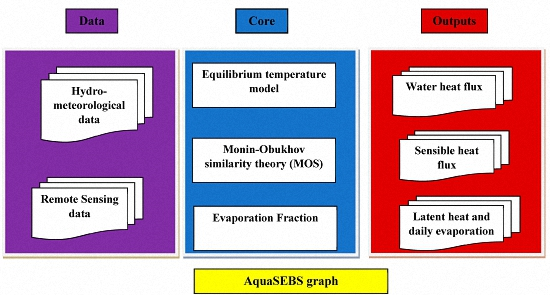
2.1. Description of the SEBS Model

The Surface Energy Balance System (SEBS) algorithm was developed by Su [3] to estimate the heat fluxes by integrating satellite data and hydro-meteorological field data. SEBS is a one-source physical model which is applicable on a large scale, as it incorporates the physical state of the surface and the aerodynamic resistances for daily evaporation estimation [6]. It has been validated in several studies over land [4,7,14,15], but has hardly been validated over fresh and saline water bodies.

SEBS requires three sets of data as input. The first set is the remote-sensing data, including emissivity, surface albedo and (water) surface temperature. The second set is the meteorological data, including air pressure, air temperature, relative humidity and wind speed at a reference height. Thirdly, radiative forcing parameters are required, such as downward shortwave and long-wave radiations.

The energy balance of the water surface can be expressed as Equation (1).

R_n = G₀ − H − λE

(1)

where R_n is the broadband net radiation, G₀ is the water (or ground for land surfaces) heat flux, H is the sensible heat flux and λE is the latent heat flux. All terms are expressed in (W·m⁻²).

The net radiation is the balance between the incoming and outgoing radiations and this is the forcing of the system energetically.

2.1.1. Heat Flux (G₀)

G₀ represents the energy used to heat the ground. Over land, G₀ is calculated as a function of the surface properties [3]. In many SEBS applications, ground and water cover is not differentiated. Simple approximation for water bodies was suggested by [9] as G₀ = 0.5 R_n (W·m⁻²). However, the measurements done over Ijsselmeer and Tana lakes showed that G₀ is not constant in space and time over a water surface.

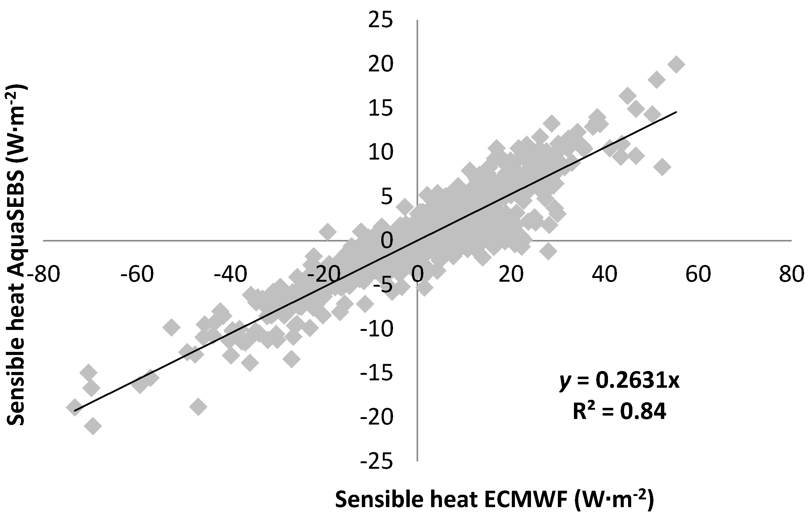
2.1.2. Sensible Heat Flux (H)

The sensible heat flux is the exchange of heat between the atmosphere and the surface through air molecules, resulting from the vertical temperature gradient between the water surface and the atmosphere. The sensible heat flux is estimated by iteration of the non-linear equations of the Monin-Obukhov Similarity (MOS) [3] (Equations (2)–(4)).

$$u=\frac{u_{*}}{k}\left[\mathit{ln}\left(\frac{z-d_0}{z_{0m}}\right)-{\phi }_m\left(\frac{z-d_0}{z_{0m}}\right)+ {\phi }_m\left(\frac{z_{0m}}{L}\right)\right]$$

(2)

$$\left({\theta }_{0 }- {\theta }_a\right)= \frac{H}{k u^{*}\rho C_p}\left[\left(\ln \left(\frac{z-d_0}{Z_{0h}}\right)-{\phi }_h\left(\frac{z-d_0}{L}\right)+{\phi }_h\left(\frac{z_{0h}}{L}\right)\right)\right]$$

(3)

$$L= \frac{\rho c_{p }{u}_{*}^2{\theta }_v}{k g H}$$

(4)

Here u is the velocity of air (m·s⁻¹); u_* is the friction velocity (m·s⁻¹); k is the von Karman’s constant (k = 0.4 (-); z is the reference height above the water surface (m); d₀ is the zero plane displacement (m); z_0m is the surface roughness length for momentum transfer (m); L is the Monin-Obukhov length (m); θ₀ is the potential temperature of the water surface (K); θ_a is the potential temperature of air at reference height z (K); z_0h is the surface roughness length for heat transfer (m); ${\phi }_m$ and ${\phi }_h$ are the stability correction functions for momentum and sensible heat transfer, respectively; is the air density (kg·m⁻³); c_p is the specific heat of air at constant pressure (J·kg⁻¹·K⁻¹); and is the gravitational acceleration g = 9.81 (m·s⁻²). These equations can be applied if the reference height is a few meters above the ground, where the surface heat fluxes are related to the atmosphere and surface variables [8]. Otherwise, Bulk Atmospheric Boundary Layer (ABL) Similarity (BAS) equations can be used [3].

2.1.3. Latent Heat (λE)

The latent heat is the energy needed for evaporation. SEBS calculates the latent heat using the evaporative fraction term (EF) and the actual sensible heat [3]. Evaporative fraction is the ratio between the latent heat and the available energy at the water surface. The daily stability of this term was investigated in different studies [7,10,15]. The actual sensible heat flux value is constrained between the dry (minimum latent heat flux) and wet (minimum sensible heat) conditions. The terms are coming from land application, where the sensible heat in dry conditions is equal to the difference between the net radiation and the ground heat flux, i.e., there is no water available for evaporation, and the soil moisture is at wilting point. In wet conditions, when there is no water limitation, the sensible heat flux reaches its minimum; and evaporation will occur at the potential (maximum) rate. SEBS estimates the total energy used for evaporation in a day-based evaporative fraction term (EF) using Equation (5) [3].

$$\lambda E_{daily}=8.64\times {10}^{7}EF (R_n-G_0 )$$

(5)

Over land, the daily ground heat flux is considered zero. However, in this paper, it is proved that this is not valid for water surfaces. So, another formulation of water heat flux is introduced to SEBS.

Finally, this total daily energy is converted into daily evaporation estimates by considering the latent heat of vaporization (λ) (Equation (6)):

$$E_{daily}=\lambda E_{daily}/\lambda {\rho }_w$$

(6)

Here, E_daily is the daily evaporation (mm·day⁻¹); ρ_w is the water density (kg·m⁻³).

2.2. Development of AquaSEBS

Based on the SEBS model as it is described in Section 2.1, we implemented modifications to estimate evaporation over water using remote sensing in the following five steps:

• Adapting the formulations of the water heat flux (G_0w).
• Identifying the roughness of momentum transfer (z_0m) for fresh water.
• Identifying the roughness of heat transfer (z_0h) for fresh waters.
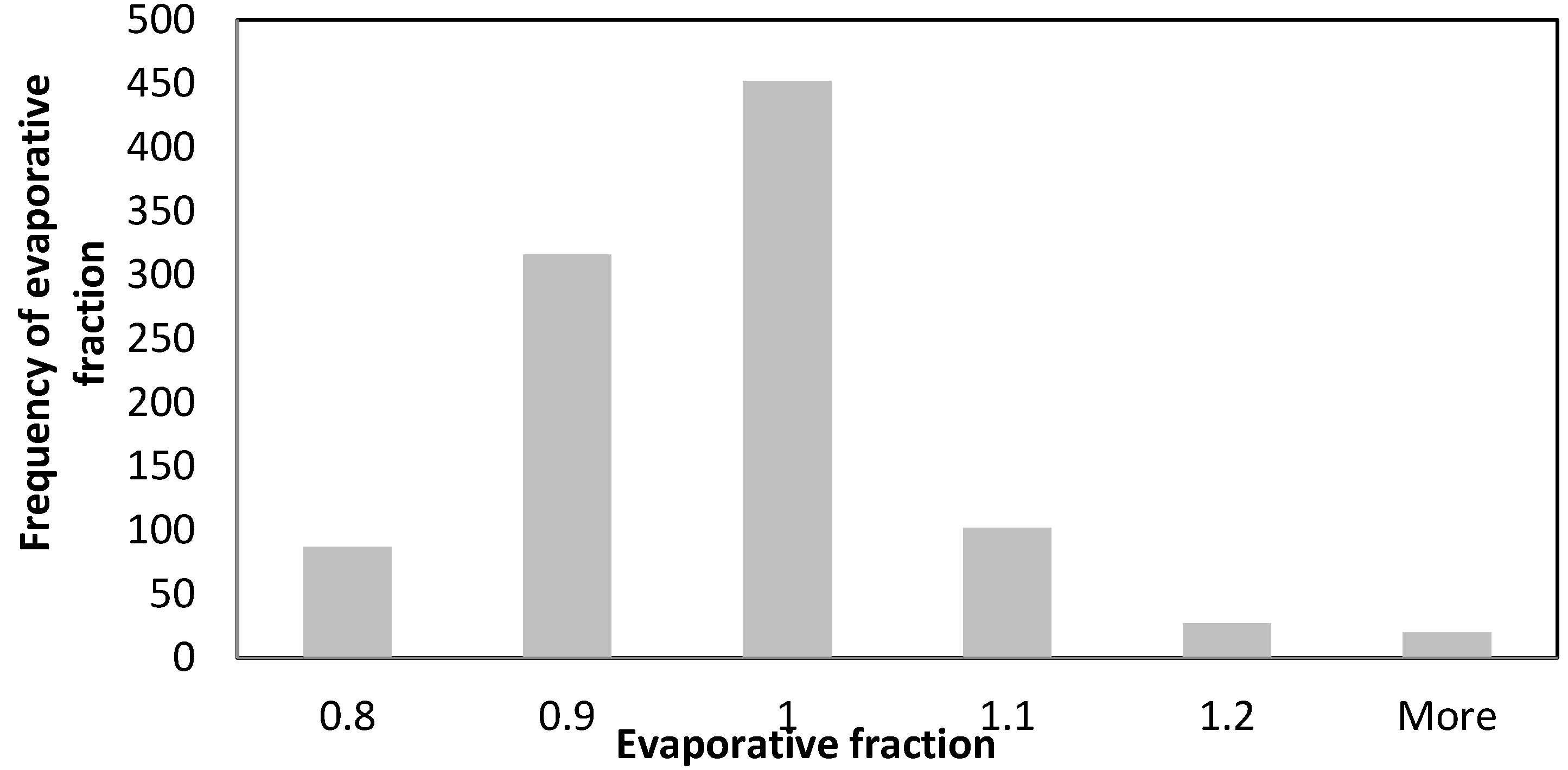
• Modifying the parameterization of the evaporative fraction to upscale the instantaneous values to daily values.
• Adding a salinity-correction term to the latent heat of vaporization.

2.2.1. Water Heat Flux (G_0w)

For the estimation of the water heat flux (denoted as G_0w to differentiate it for the ground heat flux), the thermal equilibrium exchange model [16] was incorporated into the SEBS model as detailed hereafter. Many studies neglect the value of water heat flux on a daily basis, as the energy gained during a daytime is assumed to be lost in the night. In reality, it depends on the atmospheric conditions and the amount of heat transported by flow and convection at the surface of the water body [11]. From in situ measurements, the water heat flux, G_0w, can be estimated from temperature measurements at different water depths [11] (Equation (7)):

$$G_{0w}= {\rho }_w{c}_w{{\displaystyle \int }}_{Z=0}^Z\frac{\Delta T}{\Delta t} dZ$$

(7)

where ΔT/Δt is the rate of change in temperature between two consecutive depths (K·s⁻¹); Z is the thickness of the water layer between two consecutive depths (m) and c_w is the specific heat of the water (J·kg⁻¹·K⁻¹).

Remote sensing observations, however, only obtain the skin temperature of the water. Consequently, direct use of Equation (7) is not possible. Instead, the equilibrium temperature model (ETM) [17] was used, as explained hereafter. Water heat flux can be described as the imbalance between the solar radiation, thermal radiation, sensible heat and latent heat fluxes. As such, there is a theoretical height at which the net heat flux exchange between the water surface and the atmosphere equals zero. The equilibrium temperature (T_e) is a hypothetical water surface temperature when this occurs. This equilibrium temperature can be calculated using the thermal exchange coefficient (β). In order to estimate the equilibrium temperature and the thermal exchange coefficient, as well as to derive the water heat flux (G_0w), Equations (8)–(13) can be applied:

$$T_n=0.5 ( T_0- T_d )$$

(8)

$$\eta =0.35+0.015 T_0+ 0.0012 {(T_n)}^2$$

(9)

$$S\left(W\right)=3.3 u$$

(10)

$$\beta =4.5+0.05 T_0+ \left(\eta +0.47\right) S(W)$$

(11)

$$T_e= T_d+\frac{R_s}{\beta }$$

(12)

$$G_{0w}= \beta \left(T_e- T_0\right)$$

(13)

where T_e is the equilibrium temperature (°C); T₀ is the water surface temperature (°C); T_d is dew temperature of the air (°C); R_s is the net shortwave radiation (W·m⁻²); β is the thermal exchange coefficient (W·m⁻²·°C⁻¹); S(W) is the wind function (m·s⁻¹). This method had been applied in various studies, (e.g., [16,18]). In this paper, we estimate the instantaneous water heat flux using the equilibrium temperature model. The input parameters to the equilibrium temperature model are water surface temperature, dew temperature, wind speed and the net solar radiation. In our case, the results were compared with the European Centre for Medium-Range Weather Forecasts (ECMWF) water heat flux values (calculated as a residual of the energy balance equation) over selected test areas.

2.2.2. The Roughness Height for Momentum Transfer (z_0m)

The roughness height for momentum transfer (z_0m) and the zero displacement height (d₀) play a vital role in the Monin-Obukhov Similarity theory (MOS) (Equations (3) and (4)). These two parameters significantly influence the momentum transfer between the evaporating surface and the atmosphere [12]; z_0m is the height up to which the momentum transfer is affected by surface characteristics [18]. Despite that this parameter is related to wind speed, atmospheric stratification and other factors, z_0m can be considered as a constant value over water bodies [19]. Although it is difficult to get an accurate estimation of z_0m, many methods have been developed to get a realistic estimation based on experimental measurements or remote-sensing techniques [20,21]. Equation (14) [22] was used to estimate the roughness for momentum in this study.

$$z_{0m}=u_{*}{}^2/81g$$

(14)

The zero displacement height (d₀) over water surface was assumed to be zero [23].

2.2.3. The Roughness Height for Heat Transfer (z_0h)

Many studies have been developed to estimate z_0h on land [20,21,24]. However, few studies have investigated it for water surfaces. In this research, z_0h was determined using eddy covariance heat fluxes and hydro-meteorological data by inverting the similarity equations. The equation of [10] was used to estimate the roughness of heat transfer on water surface (Equations (15) and (16)).

$$k{B}^{-1}= {\rho }_a{c}_p\frac{\left(T_0-T_a\right)}{H}k{u}^{*}-\mathit{ln}\left[\frac{z-d_0}{z_{0m}}\right]+{\phi }_h\left(\frac{z-d_0}{L}\right)$$

(15)

$$k{B}^{-1}= \mathit{ln}\frac{z_{0m}}{z_{0h}}$$

(16)

where, B is the Stanton number (-); T_a is the air temperature (K). As the roughness height for heat transfer can be considered constant over water surfaces [25], the values obtained over the Lake IJsselmeer were used also for larger water bodies.

2.2.4. Up-Scaling to Daily Values

In the original (land) SEBS, the evaporative fraction is calculated using the sensible heat values at dry and wet boundary conditions (Equation (17)).

$$EF=\lambda E_{wet}\left(\frac{E{F}_r}{(R_n-G_0)}\right)$$

(17)

where ${\mathrm{EF}}_{\mathrm{r}}$ is the relative evaporative fraction (-) which can be calculated using Equation (18). $\mathsf{\lambda }{\mathrm{E}}_{\mathrm{wet}}$ is the latent heat under wet condition where the potential evapotranspiration takes place and the sensible heat takes its minimum value $({\mathrm{H}}_{\mathrm{wet}})$.

$$E{F}_r= \frac{\lambda E}{\lambda E_{wet}}=1- \frac{\lambda E_{wet}-\lambda E}{\lambda E_{wet}}=1-\frac{H- H_{wet}}{H_{dry}- H_{wet}}$$

(18)

where ${\mathrm{H}}_{\mathrm{dry}}$ is the sensible heat under the dry condition where the evapotranspiration takes its minimum value.

This evaporative fraction is used to scale from instantaneous to daily values. However, the underlying assumptions for the use over land and water differ. The difficult question is how to consider conceptually the dry boundary over water surfaces. For relative humidity higher than 70%, no evaporation will take place over the water that is saturated with sodium or magnesium chloride [26]. Therefore, the evaporation process above the water surface is constrained by the water composition and the atmospheric conditions. In this work, the dry condition was considered for salt-saturated water and relative air humidity >70%, whereas, the ‘wet’ condition was considered over open fresh water.

2.2.5. Correction for Salinity

The influence of salinity on the latent heat of vaporization and evaporation rate is expressed as a reduction of evaporation of saline water in comparison to fresh water. We use the salinity reduction formulation of [27], (Equation (19)).

$$\propto =1.025 - 0.0246\mathit{exp}\left[0.00879·s\right]$$

(19)

where ∝ is the salinity reduction factor, is the salinity (g·L⁻¹). Equation (20) is used to correct for salinity effect on the daily evaporation rate produced by AquaSEBS.

$$E_s= \propto \lambda E_{daily}/\lambda {\rho }_w$$

(20)

where $E_s$ is the estimated evaporation rate over the surface of the saline water body.

3. Data Collection and Analysis

In this study, we used three data sets, two sets were measured in inland waters and one set is based on ECMWF ERA-Interim reanalysis. To make an objective evaluation of the improvements to the SEBS model, we chose to use the meteorological forcing data from ECMWF to run both SEBS and AquaSEBS and validated the results using in situ measurements (Lake IJsselmeer and Lake Tana) and using ECMWF ERA-Interim data where in situ measurements were not available.

Lake IJsselmeer, The Netherlands: A measurement setup was constructed at the shore of Lake IJsselmeer for calibration and validation purposes. The set up consisted of water temperature profile measurements and a flux tower. The tower had a 4-component radiation sensor, an eddy-covariance sensor, and a relative humidity sensor. The eddy-covariance sensor was installed at 3 m height whereas the relative humidity sensor was at 2 m height. The radiation sensors were installed at 1.5 m height above the water surface, and 4 m away from the land. The water surface temperature was calculated from the measured radiation data using the Stefan-Boltzmann equation.

Lake Tana, Ethiopia: Data from Lake Tana were used for evaluating the calibrated roughness heights. At this location temperature profile at different depths in the water and air, wind speed, relative humidity, and net radiation components were collected during the one-day period of 15–16 September 2011 [11,28].

ECMWF products: ECMWF ERA-Interim reanalysis data products, provided by the European Centre for Medium Range Weather Forecasts organization, were used as reference data to validate AquaSEBS over different test areas. It has to be noted that these data products can be considered as the best fit of world-wide in situ measurements and modelled data, since this data set is energetically consistent.

3.1. Processing the IJsselmeer Data

All measured values, including the four components of radiation, air temperature, and relative humidity, were averaged to 30 min intervals. The footprint of the eddy co-variance sensor was computed following [29]. More than 70% of the measured evaporation came from the surrounding 150 m of the eddy co-variance sensor. Three scenarios were identified in the dataset, according to the source of the signal, i.e., the footprint: full water, full land and mixed fetch. The data were then filtered to consider only the fluxes over the water. This occurred when the wind direction was between 200° and 280°.

3.2. Analysis

The GeoCalVal method [30] was used to divide the collected data into two independent sets for calibration and validation. The calibration (Cal) set was used to infer the values of the water heat flux and roughness heights for heat and momentum, whereas the validation (Val) set was used to check the accuracy of AquaSEBS in producing the energy balance terms (evaporation and sensible heat). AquaSEBS was evaluated at different spatial scales over different study areas with various salinity concentrations (

Table 1. Latitude, longitude and salinity of each study area.

Study Area	Corners of the Area		Salinity (g·L−1)	Descriptor
	Upper Right	Lower Left
Great Salt Lake	41°30′00″N	40°45′00″N	240 [31]	Brine
	111°45′00″W	112°30′00″W
Atlantic Ocean	24°30′00″N	23°30′00″N	34.7 [1]	Saline
	39°30′00″W	40°30′00″W
Indian Ocean	18°30′00″S	19°30′00″S	34.7 [1]
	74°30′00″E	73°30′00″E
Mediterranean Sea	33°30′00″N	32°30′00″N	34.7 [1]
	26°30′00″E	25°30′00″E
North Sea	60°30′00″N	59°30′00″N	34.7 [1]
	00°30′00″E	00°30′00″W
Red Sea	18°30′00″N	17°30′00″N	34.7 [1]
	39°30′00″E	38°30′00″E
IJsselmeer lake	52°49′00″N	52°49′00″N	0.6 [32]	Brackish
	5°15′00″E	5°15′00″E
Lake Victoria	00°30′00″S	01°30′00″S	0.17 [33]	Fresh
	33°30′00″E	32°30′00″E
Lake Tana	37°30′00″S	37°30′00″S	0.143 [34]
	12°00′00″E	12°00′00″E

).

Various statistical parameters were used to assess the efficiency of the model on the evaporation rate estimation such as average, standard deviation (STD), root mean square error (RMSE) (Equation (21)) and relative root mean square error (rRMSE) (Equation (22)).

$$RMSE= \sqrt{n^{-1}{\displaystyle \sum }_{i=1}^n{\left(X_i- Y_i\right)}^2}$$

(21)

$$rRMSE=100\times RMSE/\left(Y_{max}- Y_{min}\right)$$

(22)

where n is the sample size, ${\mathrm{X}}_{\mathrm{i}}$ is the model estimated parameter; ${\mathrm{Y}}_{\mathrm{i}}$ is the measured reference value; ${\mathrm{Y}}_{\max }$ and $Y_{min}$ are maximum and minimum of the reference values, respectively.

4. Results and Discussions

4.1. Water Heat Flux

Table 2. Comparison of water heat flux values calculated by AquaSEBS (using the equilibrium temperature model) and ECMWF models (January 2010 to September 2012).

Area	Indian Ocean		Atlantic Ocean		Mediterranean Sea		North Sea		Red Sea
Model	AquaSEBS	ECMWF	AquaSEBS	ECMWF	AquaSEBS	ECMWF	AquaSEBS	ECMWF	AquaSEBS	ECMWF
n	1005	1005	1005	1005	1005	1005	1005	1005	974	974
Average (W·m−2)	126.5	120.0	53.7	55.7	507.5	513.8	101.1	147.7	573.3	542.7
STD (W·m−2)	180.5	175.1	131.6	131.8	284.8	253.8	284.2	252.5	132.5	136.3
RMSE (W·m−2)	32.2		26.5		49.6		68.5		42.1
rRMSE (%)	4.8		4.3		5.2		8.5		6.4

shows the resulting water heat flux from AquaSEBS after applying the equilibrium temperature model. Comparison with ECMWF data shows that the computed $G_{0w}$ values are in close agreement with ECMWF outputs with less than 9% of rRMSE.

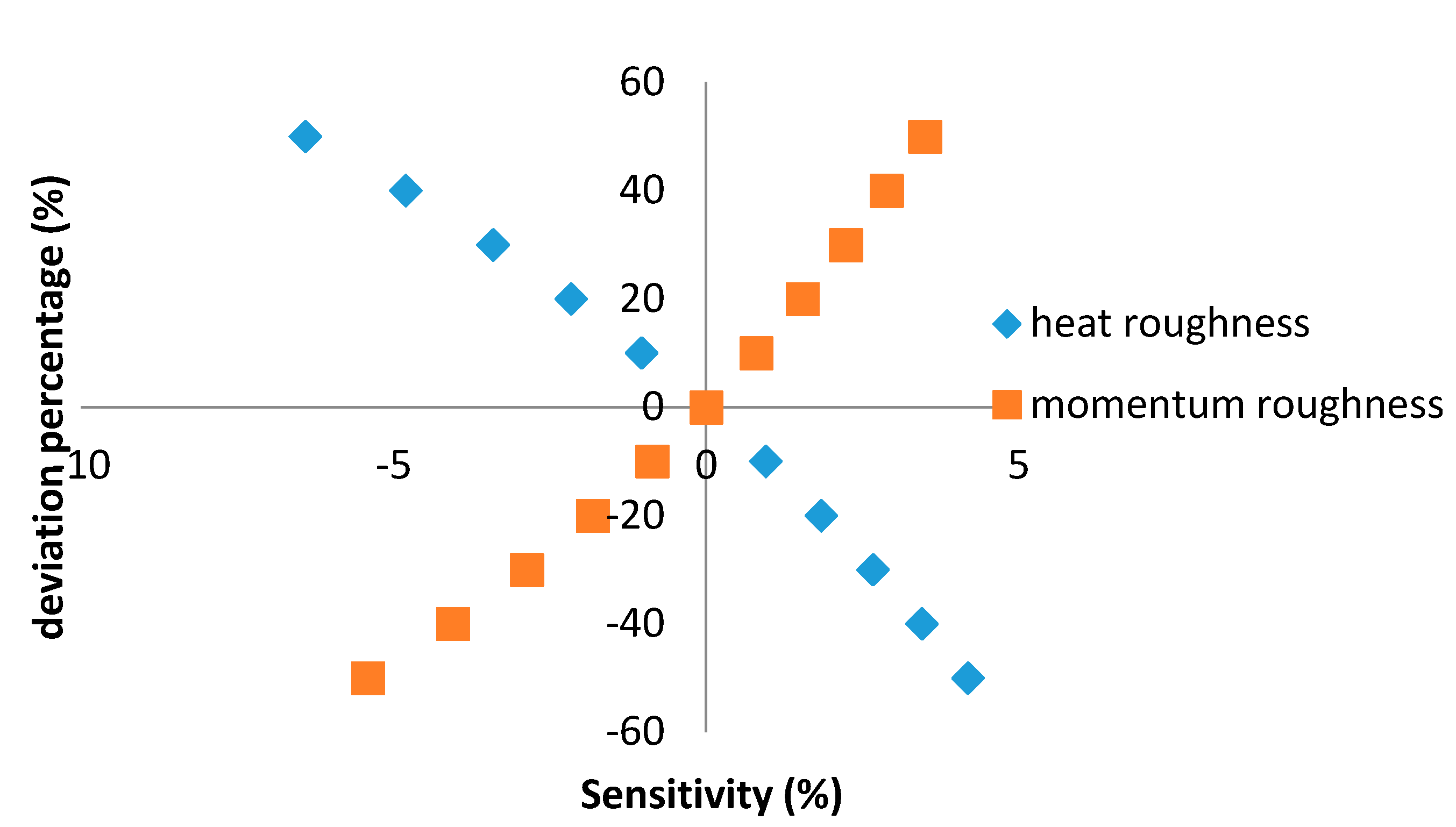
4.2. Momentum and Heat Transfer Roughness Heights

The roughness of momentum transfer, $z_{0m}$ was computed as 0.0002 m. This small value of $z_{0m}$ means that the momentum transfer to the atmosphere is close to the water surface. The roughness height for heat transfer parameter over a water surface was estimated to be 0.0001 m, whereas the sensible heat ranges between −70 W·m⁻² and 30 W·m⁻².

The estimated roughness height parameters were used to estimate the sensible heat over IJsselmeer lake using AquaSEBS model for the period of 11–26 October 2012. The results show similarity between AquaSEBS heat fluxes and the eddy covariance heat fluxes data (Figure 1) with RMSE of 9.0 W·m⁻² and R² = 0.70.

The low difference between the roughness height for momentum transfer and its counterpart for heat transfer is reflected in the kB⁻¹ value. It is estimated to be 0.3 over water surfaces. It is notable that the roughness height for heat transfer is less than for the momentum transfer. In other words, the level of virtual source of heat is lower than the level of the virtual sink for momentum; therefore, the aerodynamic resistance of heat transfer is larger than of momentum transfer [10].

Although [10] stated that the poorest estimation of sensible heat flux takes place when the difference between the roughness lengths is small, AquaSEBS produces good estimations of the sensible heat. This is due to the iteration process of the similarity relationship between the sensible heat, friction velocity and Monin-Obukhov length, which improves the accuracy of the estimates. In addition, AquaSEBS shows lower sensitivity to the roughness parameters over water surfaces than to the atmospheric parameters (see Section 4.6).

Eddy covariance data measured at the IJsselmeer site were used to estimate the aerodynamic resistance parameters, including the roughness height values of momentum and heat transfer. It was found that the aerodynamic resistance of the water surface relates to the wind speed in an inverse exponential relationship. Therefore, an increase in the wind speed value leads to a decrease of the aerodynamic resistance of water. Above 3 m·s⁻¹ wind speed, the aerodynamic resistance over water surfaces ranges mostly between 50 and 200 s·m⁻¹, resulting in low sensible heat fluxes.

4.3. Daily Evaporation

It was found that the average daily evaporative fraction over the Mediterranean Sea in the period between January 2010 and September 2012 had mostly high values, as most of the available energy was converted to latent heat. The histogram in Figure 2 illustrates that the evaporative fraction ranges mostly between 0.8 and 1.2. Values lower than 1.0 occur when sensible heat has a positive value (unstable condition), and higher than 1.0 occur when the sensible heat has a negative value (stable condition). The latent heat under stable conditions dissipates energy from the stored heat in the water body. In the same regard, the ratio between the latent heat and the available energy at the surface is mostly higher than 0.8, i.e., more than 80% of the available energy at the water surface during the day is used in the evaporation process (Figure 3). The standard deviation of evaporative fraction was found to be 0.05, which confirms the stability of this parameter under different atmospheric conditions. This can be explained in terms of stability of the latent heat and available energy over the water surfaces throughout the day [35]. It can therefore be deduced that the evaporative fraction defined at overpass time of the satellite can be used to upscale evaporation rate estimation from instantaneous to a daily basis over water surfaces.

SEBS uses the evaporative fraction and daily available energy to upscale the latent heat from instantaneous to a daily basis. According to [35], the sensible and latent heat fluxes are stable during the day over water surfaces; therefore, the available energy follows a constant behavior during the day (Figure 4). AquaSEBS uses the same theory to upscale the latent heat from instantaneous to a daily basis.

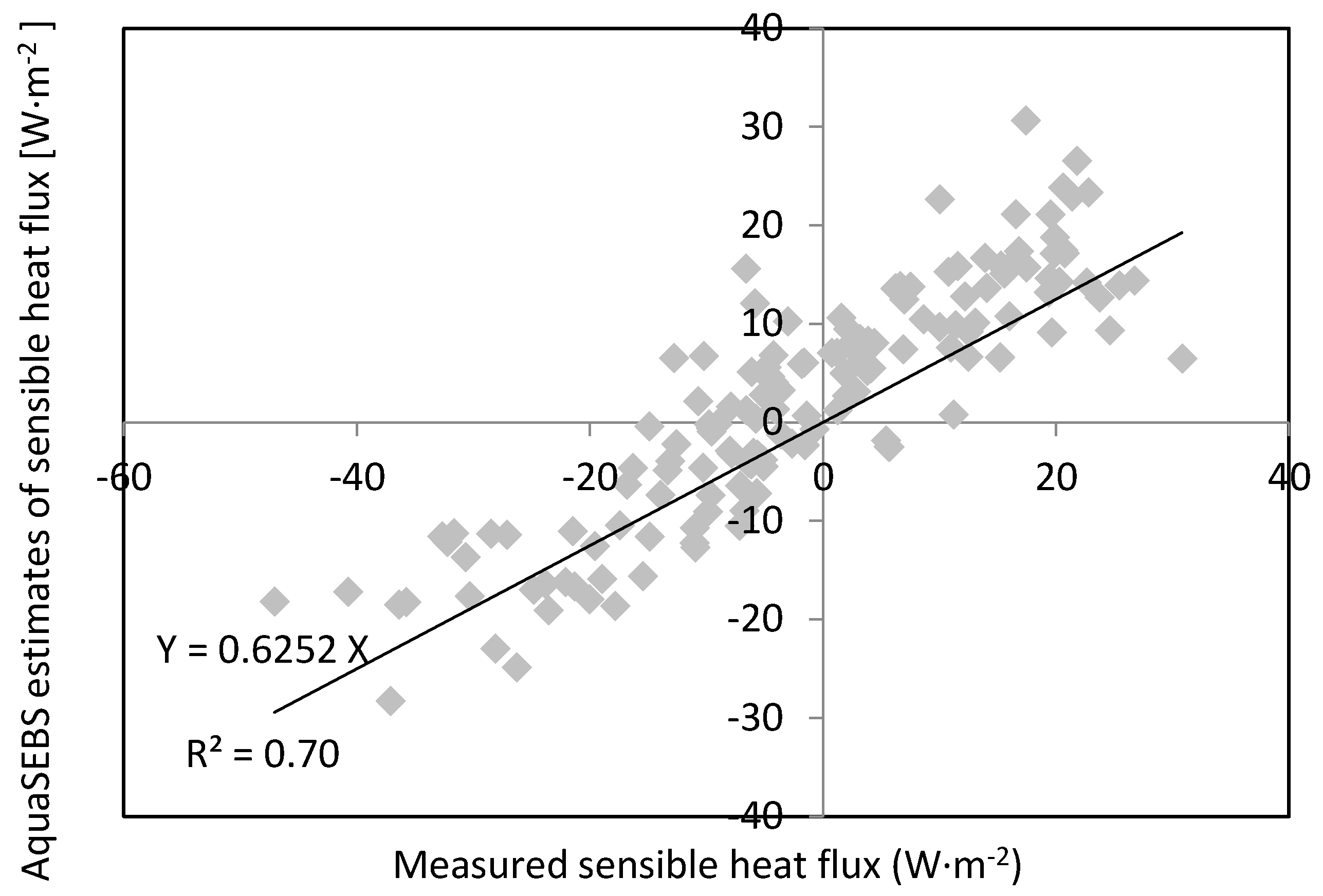
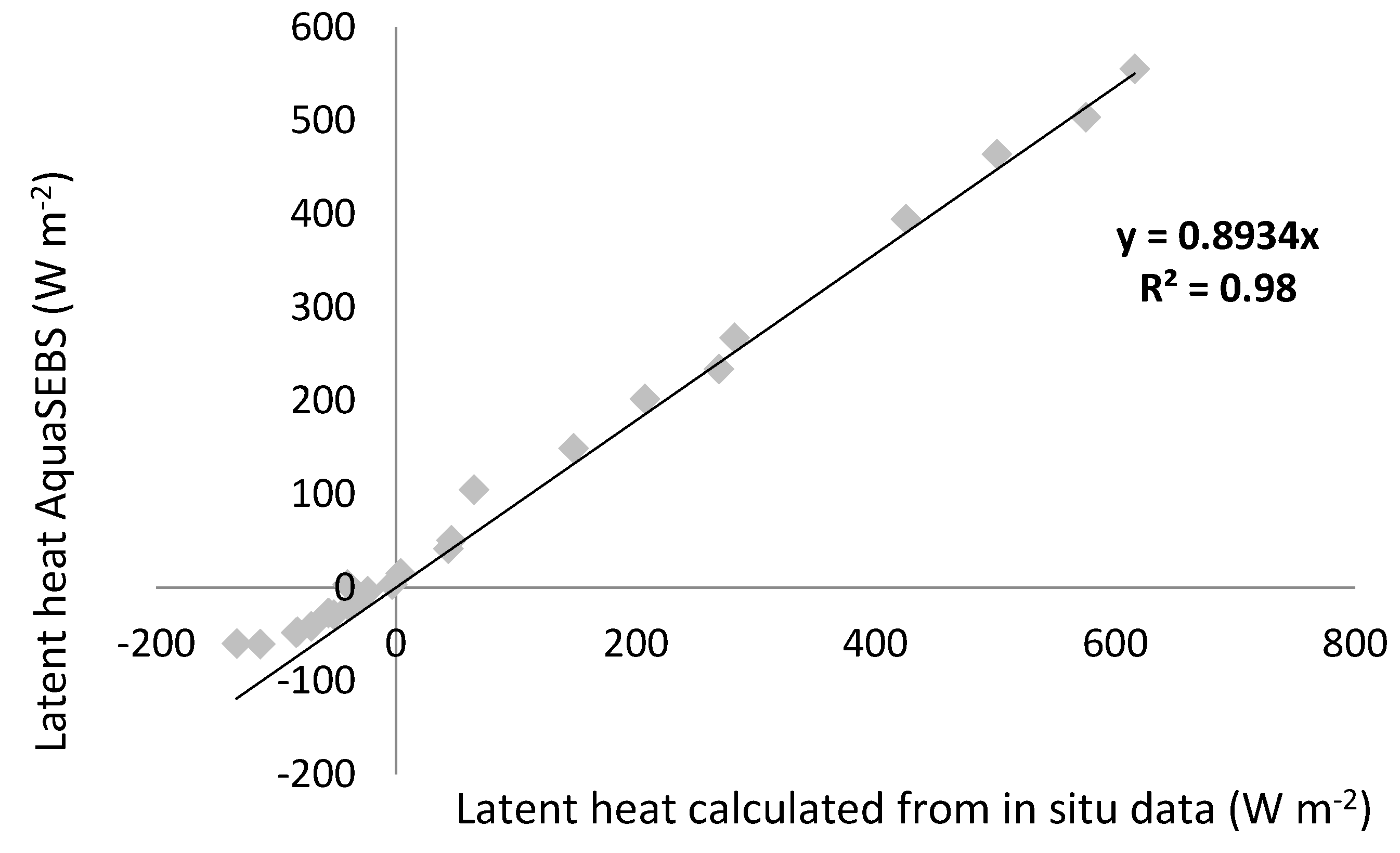
4.4. Evaluation of AquaSEBS over Fresh Water

In order to assess its performance, the AquaSEBS model has been applied to two study areas under different atmospheric conditions and at different spatial and temporal scales. Ground data and ECMWF data were used to validate the model over the Tana and Victoria lakes, respectively.

For Lake Tana, the latent heat and the sensible heat flux values calculated by AquaSEBS were compared to the ones calculated by [11] using field measurements of four component radiation (CNR1, Kipp and Zonen), Bowen ratio (inter-calibrated Theodor Friedrichs TRH sensors at two heights), water temperature (Onset TMC20-HD) and eddy covariance (CSAT3 sonic anemometer, Campbell Scientific Inc., Logan, UT, USA). Both fluxes show a good agreement (Figure 5 and

Table 3. Comparison of the AquaSEBS results and heat fluxes calculated from field measurements over Lake Tana by [11] (W·m⁻²).

	LE (AquaSEBS) (W·m−2)	LE (in Situ by [11]) (W·m−2)	H (AquaSEBS) (W·m−2)	H (in Situ by [11]) (W·m−2)
n	23	23	23	23
Average (W·m−2)	102.1	109.9	21.6	21.1
STD (W·m−2)	226.3	193.8	13.7	17.2
RMSE (W·m−2)	35.6		4.8
rRMSE %	10.3		7.9

). It can be seen that the AquaSEBS model exhibits a slight underestimation compared to the in situ data during the night time, i.e., when the net radiation is negative.

It is interesting to note that while over the Indian Ocean the latent heat flux was practically constant during a day (Figure 4), over Lake Tana it showed a diurnal variation (Figure 5). Figure 4 demonstrates that over oceans, convection dissipates the incoming energy, thus the heat fluxes towards the air remain relatively stable, or in fact, change very slowly. The dissipated energy modifies the thickness of the convection layer of the ocean. In an inland (shallow) lake, water depth influences the amount of energy stored since the possible thickness of the convection layer is limited to the water depth. This affects the latent heat and sensible heat fluxes, resulting in diurnal variations, as shown by Figure 5.

The AquaSEBS model was implemented over Lake Victoria. No ground data were available during the execution of this research; therefore, ECMWF simulated data were used for input. There was a good agreement between AquaSEBS estimates of sensible heat, latent heat, water heat flux as well as daily evaporation rate values and the corresponding ECMWF variables (

Table 4. Comparison between the AquaSEBS model and ECMWF model over Lake Victoria (January 2010 to September 2012).

	Water Heat Flux (W·m−2)		Sensible Heat (W·m−2)		Latent Heat (W·m−2)		Daily Evaporation (mm·day−1)
	AquaSEBS	ECMWF	AquaSEBS	ECMWF	AquaSEBS	ECMWF	AquaSEBS	ECMWF
n	1005	1005	1005	1005	1005	1005	1005	1005
Average (W·m−2)	110.2	110.9	3.9	4.2	51.4	51.0	4.8	4.8
STD (W·m−2)	82.8	79.3	4.63	5.02	34.09	29.59	2.8	1.7
RMSE (W·m−2)	19.9		1.7		19.8		1.5
rRMSE (%)	6.7		4.1		8.9		7.4

).

4.5. Salinity Effect

Water salinity reduces the evaporation due to a decrease in the saturation vapor pressure and an only partially compensating increase in water surface temperature [36]. The effect is very limited (less than 1% reduction in evaporation) for fresh and brackish water (0–20 g·L⁻¹), and increases gradually over saline and hypersaline water reaching ~32% (reduction) for salinity up to 300 g·L⁻¹. AquaSEBS is applied over different geographic areas at one square degree grid to estimate the daily evaporation from January 1979 to December 2012. The mean global salinity of the oceans is 34.7 g·L⁻¹ [1].

It can be shown that the evaporation calculated by the AquaSEBS model (accounting salinity) corresponds to the ECMWF data very well (

Table 5. Comparison between the evaporation rate values calculated by the AquaSEBS and ECMWF models (January 2010 to September 2012).

	Atlantic Ocean			Indian Ocean
	Aqua SEBS	AquaSEBS (accounting salinity)	ECMWF	Aqua SEBS	AquaSEBS (accounting salinity)	ECMWF
n	1005	1005	1005	1005	1005	1005
Average (mm·d−1)	5.04	5.01	5.01	6.95	6.81	6.72
STD (mm·d−1)	1.88	1.86	1.85	2.70	2.68	2.63
RMSE (mm·d−1)	0.11	0.10		0.25	0.21
rRMSE (%)	0.90	0.81		1.44	1.27

). In both cases, AquaSEBS (without accounting salinity) overestimated the evaporation, and the introduced parameterization and salinity coefficient decrease it to match the ECMWF values. AquaSEBS estimates of heat fluxes have been validated with ECMWF data (

Table 6. Comparison of the heat fluxes values calculated by the AquaSEBS and ECMWF models over Lake Victoria (January 2010 to September 2012).

	Water Heat Flux (W·m−2)		Sensible Heat (W·m−2)		Latent Heat (W·m−2)		Daily Evaporation (mm·d−1)
	AquaSEBS	ECMWF	AquaSEBS	ECMWF	AquaSEBS	ECMWF	AquaSEBS	ECMWF
n	1005	1005	1005	1005	1005	1005	1005	1005
Average	110.2	110.9	3.9	4.2	51.4	51.0	4.8	4.8
STD	82.8	79.3	4.63	5.02	34.09	29.59	2.8	1.7
RMSE	19.9		1.7		19.8		1.5
rRMSE (%)	6.7		4.1		8.9		7.4

).

Since the RMSE of the water heat flux is much higher than that of the sensible heat, it can be concluded that the overall uncertainty of the model output propagates from errors in the water heat flux estimation.

The deviation between the two models over different study areas is less than 20 W∙m⁻². The accuracy of the AquaSEBS computation of sensible heat flux was tested under different atmospheric and stability conditions: wind speeds between 0.07 and 20 m∙s⁻¹, and temperature difference of air-water between −4 and 8.5 °C. Overestimation occurs between the two models when the wind speed is higher than 10 m·s⁻¹ and the temperature difference is larger than 4 °C, whereas underestimation occurs for the same wind speed and negative temperature difference of −2 °C. This may be due to the inability of the stability equations to describe the boundary layer of a roughened sea surface.

The estimated latent heat closely follows the values of ECMWF data at most test sites (

Table 7. Comparison of the latent heat values calculated by the AquaSEBS and ECMWF models (January 2010 to September 2012).

	Atlantic Ocean		Indian Ocean		Mediterranean Sea		Red Sea		North Sea
	AquaSEBS	ECMWF	AquaSEBS	ECMWF	AquaSEBS	ECMWF	AquaSEBS	ECMWF	AquaSEBS	ECMWF
n	1005	1005	1005	1005	1005	1005	974	974	1005	1005
Average (W·m−2)	151.1	145.1	181.7	194.6	120.9	120.5	100.8	128.6	101.1	57.1
STD (W·m−2)	55.9	56.7	79.7	78.5	103.8	77.7	63.0	68.7	94.3	54.1
RMSE (W·m−2)	26.9		33.7		51.1		37.6		77.5
rRMSE (%)	6.8		7.0		8.6		10.5		14.3

). The maximum average rRMSE is 14.3% over the North Sea, where the net shortwave radiation and the dew temperature are low, the temperature difference has a low negative value, and the wind speed value is high; resulting in a high error in the water heat flux and sensible heat estimation, thus in the latent heat estimation.

To test the model over a hypersaline water body, the AquaSEBS model was applied over the Great Salt Lake in the US and was compared to the ECMWF water heat flux values. Other hypersaline water bodies, such as the Dead Sea in Jordan, could not be investigated due to the small size of the lake relative to the large pixel size of the ECMWF data products.

The comparison over the Great Salt Lake shows a clear improvement in the instantaneous evaporation estimation by the AquaSEBS model in comparison to the original SEBS model with about a 4% reduction in rRMSE and 0.25 mm 3 h⁻¹ (

Table 8. Comparison of evaporation rates calculated by different models over the Great Salt Lake in the period of (January 2010 to September 2012).

Statistical tools	SEBS	AquaSEBS	ECMWF
Average (mm 3 h−1)	0.78	0.57	0.26
STD (mm 3 h−1)	0.51	0.37	0.20
RMSE (mm 3 h−1)	0.63	0.38
rRMSE (%)	23.48	19.60

). AquaSEBS over the Great Salt Lake reduces the calculated evaporation by 26.5% under the same atmospheric conditions, but it is still higher than the ECMWF-calculated values. The sensible heat fluxes over saline water are larger than over freshwater. Thus, an underestimation of sensible heat is observed between AquaSEBS and ECMWF results, as shown in (Figure 6). The mean values of sensible heat for the two models are 20.52 W·m⁻² and 94.42 W·m⁻², respectively, and the slope of the linear equation is 0.26. This low slope value is due to the conversion of the excess energy from the reduced evaporation to other heat fluxes [37]. As it was described in Section 4.4, in oceans, most of this energy is converted to water heat flux resulting in an increase of the convection layer thickness [38]. In inland lakes, shallow water depth limits the thickness of the convection layer, thus it affects the heat fluxes [39]. At this stage, the effect of (shallow) water depth is not directly considered in AquaSEBS.

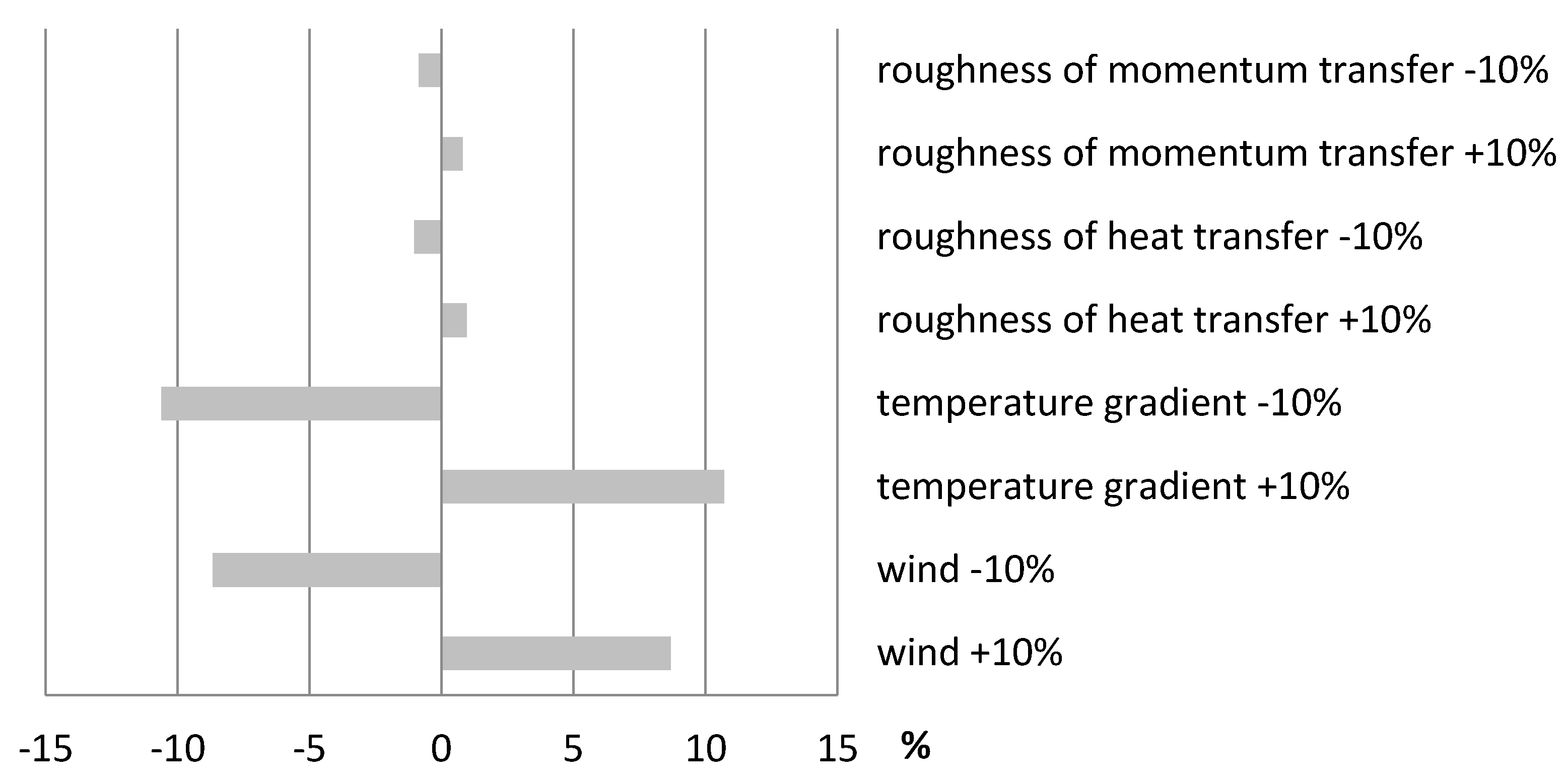
4.6. Evaluation and Sensitivity Analysis

To evaluate the model sensitivity, we estimated the effects of the variability of the values of each important input parameter. We showed that a high error in the water heat flux estimation greatly affects the performance of the AquaSEBS model. We found that the modelled water heat flux is more sensitive to the surface water temperature than to other parameters. In general, the most - to - least effectual parameters on the water heat flux value are the water surface temperature, dew temperature and wind speed, respectively.

The modelled sensible heat flux is more sensitive to the air temperature and wind speed than to the parameters of aerodynamic resistance. Figure 7 shows that the temperature difference is the main variable that controls the sensible heat over water surfaces. It was found that the influence of roughness height of momentum and heat on the modelled sensible heat does not exceed 6.5% when the roughness parameters are within 50% of their actual values (Figure 8).

The sensitivity of evaporation rate to errors in salinity measurements depends on the actual salinity concentration of the water body. If the salinity is estimated with an error of 10 g∙L⁻¹ at an actual concentration of 290 g∙L⁻¹, the error in the evaporation estimation will be around 2.65%, whilst a 10 g∙L⁻¹ overestimate or underestimate at 20 g∙L⁻¹ results in an error of 0.23% approximately.

5. Conclusions

Salinity is one of the parameters that affects the evaporation rate. In this study, AquaSEBS model was developed based on the SEBS surface energy balance model to estimate the heat fluxes over fresh and saline water bodies. Firstly, the equilibrium thermal exchange method was incorporated to estimate the water heat flux parameter. Secondly, the roughness heights for momentum and heat transfer were estimated as 0.0002 m and 0.0001 m, respectively. It was proved that the evaporative fraction can be assumed stable during the day. Consequently, the evaporative fraction can be multiplied by the available energy at the overpass time of the satellite to estimate the daily latent heat and evaporation. AquaSEBS was validated over different study areas with different salinity concentrations. The results showed that AquaSEBS can be used to estimate the heat fluxes and the daily evaporation over water bodies of different salinity at different spatial scales. In the presence of salinity, a part of the energy available for evaporation is converted into other forms of heat fluxes. In inland waters, this energy affects the aerodynamic resistance of the water surface (by changing the physical properties of the surface water) and increases the sensible heat fluxes. Determining the roughness heights for momentum and heat transfer over hypersaline lakes may improve the performance of the model. AquaSEBS is most sensitive to water surface temperature, therefore, satellite sensors with high thermal accuracy (<0.3 K), e.g., the ATSR, provide the most suitable input data for AquaSEBS.

References

1. Williams, P.D.; Guilyardi, E.; Madec, G.; Gualdi, S.; Scoccimarro, E. The role of mean ocean salinity in climate. Dyn. Atmos. Oceans 2010, 49, 108–123. [Google Scholar] [CrossRef]
2. Shoko, C.; Clark, D.J.; Mengistu, M.G.; Bulcock, H.; Dube, T. Estimating spatial variations of total evaporation using multispectral sensors within the uMngeni catchment, South Africa. Geocarto Int. 2016, 31, 256–277. [Google Scholar] [CrossRef]
3. Su, Z. The Surface Energy Balance System (SEBS) for estimation of turbulent heat fluxes. Hydrol. Earth Syst. Sci. 2002, 6, 85–99. [Google Scholar] [CrossRef]
4. Jia, L.; Su, Z.; van den Hurk, B.; Menenti, M.; Moene, A.; De Bruin, H.A.; Yrisarry, J.J.B.; Ibanez, M.; Cuesta, A. Estimation of sensible heat flux using the Surface Energy Balance System (SEBS) and ATSR measurements. Phys. Chem. Earth Parts A/B/C 2003, 28, 75–88. [Google Scholar] [CrossRef]
5. Rwasoka, D.T.; Reyes-Acosta, J.L.; van der Tol, S.C.Z.; Lubczynski, M.W. Evapotranspiration in water limited environments: Up-scaling from the crown canopy to the eddy flux footprint + poster. In Proceedings of the EGU General Assembly, Vienna, Austria, 2–7 May 2010.
6. Su, Z.; Pelgrum, H.; Menenti, M. Aggregation effects of surface heterogeneity in land surface processes. Hydrol. Earth Syst. Sci. 1999, 3, 549–563. [Google Scholar] [CrossRef]
7. Rwasoka, D.T.; Gumindoga, W.; Gwenzi, J. Estimation of actual evapotranspiration using the Surface Energy Balance System (SEBS) algorithm in the Upper Manyame catchment in Zimbabwe. Phys.Chem. Earth 2011, 36, 736–746. [Google Scholar] [CrossRef]
8. Brutsaert, W. Aspects of bulk atmospheric boundary layer similarity under free-convective conditions. Rev. Geophys. 1999, 37, 439–451. [Google Scholar] [CrossRef]
9. Jia, L.; Xi, G.; Liu, S.; Huang, C.; Yan, Y.; Liu, G. Regional estimation of daily to annual regional evapotranspiration with MODIS data in the Yellow River Delta wetland. Hydrol. Earth Syst. Sci. 2009, 13, 1775–1787. [Google Scholar] [CrossRef]
10. Liu, S.M.; Lu, L.; Mao, D.; Jia, L. Evaluating parameterizations of aerodynamic resistance to heat transfer using field measurements. Hydrol.Earth Syst. Sci. 2007, 11, 769–783. [Google Scholar] [CrossRef]
11. Abreham Kibret, A. Open Water Evaporation Estimation Using Ground Measurements and Satellite Remote Sensing: A Case Study of Lake Tana, Ethiopia; ITC: Enschede, The Netherlands, 2009; p. 97. [Google Scholar]
12. Koloskov, G.; Mukhamejanov, K.; Tanton, T.W. Monin-Obukhov length as a cornerstone of the SEBAL calculations of evapotranspiration. J. Hydrol. 2007, 335, 170–179. [Google Scholar] [CrossRef]
13. Tian, X.; Li, Z.Y.; van der Tol, C.; Su, Z.; Li, X.; He, Q.S.; Bao, Y.F.; Chen, E.X.; Li, L.H. Estimating zero-plane displacement height and aerodynamic roughness length using synthesis of LiDAR and SPOT-5 data. Remote Sens. Environ. 2011, 115, 2330–2341. [Google Scholar] [CrossRef]
14. Xiong, J.; Wu, B.F.; Yan, N.N.; Zeng, Y.A.; Liu, S.F. Estimation and Validation of Land Surface Evaporation Using Remote Sensing and Meteorological Data in North China. IEEE J. Sel. Top. Appl. Earth Obs. Remote Sens. 2010, 3, 337–344. [Google Scholar] [CrossRef]
15. Elhag, M.; Psilovikos, A.; Manakos, I.; Perakis, K. Application of the SEBS Water Balance Model in Estimating Daily Evapotranspiration and Evaporative Fraction from Remote Sensing Data over the Nile Delta. Water Resour. Manag. 2011, 25, 2731–2742. [Google Scholar] [CrossRef]
16. Abualnaja, Y. Estimation of the Net Surface Heat Flux in the Arabian Gulf Based on the Equilibrium Temperature. J. King Abdulaziz Univ. 2009, 20, 21–29. [Google Scholar] [CrossRef]
17. Edinger, J.E.; Duttweiler, D.W.; Geyer, J.C. The Response of Water Temperatures to Meteorological Conditions. Water Resour. Res. 1968, 4, 1137–1143. [Google Scholar] [CrossRef]
18. Ahmad, F.; Sar, S. Equilibrium temperature as a parameter for estimating the net heat-flux at the air-sea interface in the central red-sea. Oceanol. Acta 1994, 17, 341–343. [Google Scholar]
19. Zhou, Y.L.; Ju, W.; Sun, X.; Wen, X.; Guan, D. Significant decrease of uncertainties in sensible heat flux simulation using temporally variable aerodynamic roughness in two typical forest ecosystems of China. J. Appl. Meteorol. Climatol. 2012, 51, 1099–1110. [Google Scholar] [CrossRef]
20. Blümel, K. A simple formula for estimation of the roughness length for heat transfer over partly vegetated surfaces. J. Appl. Meteorol. 1999, 38, 814–829. [Google Scholar] [CrossRef]
21. Yang, R.; Friedl, M.A. Determination of roughness lengths for heat and momentum over boreal forests. Bound.-Layer Meteorol. 2003, 107, 581–603. [Google Scholar] [CrossRef]
22. Tanny, J.; Cohen, S.; Assouline, S.; Lange, F.; Grava, A.; Berger, D.; Teltch, B.; Parlange, M.B. Evaporation from a small water reservoir: Direct measurements and estimates. J. Hydrol. 2008, 351, 218–229. [Google Scholar] [CrossRef]
23. Brutsaert, W.H. Evaporation into the Atmosphere—Theory, History, and Applications; Springer: Dordrecht, The Netherlands, 1982; p. 297. [Google Scholar]
24. Su, Z.; Schmugge, T.; Kustas, W.P.; Massman, W.J. Evaluation of two models for estimation of the roughness height for heat transfer between the land surface and the atmosphere. J. Appl. Meteorol. 2001, 40, 1933–1951. [Google Scholar] [CrossRef]
25. Cahill, A.T.; Parlange, M.B.; Albertson, J.D. On the Brutsaert temperature roughness length model for sensible heat flux estimation. Water Resour. Res. 1997, 33, 2315–2324. [Google Scholar] [CrossRef]
26. Leaney, F.; Christen, E. Evaluating Basin Leakage Rate, Disposal Capacity and Plume Development; CRC for Catchment Hydrology: Monash, Vic, Australia, 2000. [Google Scholar]
27. Turk, L.J. Evaporation of Brine: A field study on the Bonneville Salt Flats, Utah. Water Resour. Res. 1970, 6, 1209–1215. [Google Scholar] [CrossRef]
28. Van der Tol, C.; University of Twente, Enschede, The Netherlands. Personal communication, 2012.
29. Kljun, N.; Calanca, P.; Rotach, M.; Schmid, H. A simple parameterisation for flux footprint predictions. Bound.-Layer Meteorol. 2004, 112, 503–523. [Google Scholar] [CrossRef]
30. Salama, M.S.; Velde, R.; Van der Woerd, H.J.; Kromkamp, J.C.; Philippart, C.J.M.; Joseph, A.T.; O'Neill, P.E.; Lang, R.H.; Gish, T.; Werdell, P.J.; et al. Technical note: Calibration and validation of geophysical observation models. Biogeosciences 2012, 9, 2195–2201. [Google Scholar] [CrossRef] [Green Version]
31. Mohammed, I.N. Modeling the Great Salt Lake, Master‘s Thesis, Utah State University, Logan, UT, USA, 2006. [Google Scholar]
32. Sollie, S.; Coops, H.; Verhoeven, J.T.A. Natural and constructed littoral zones as nutrient traps in eutrophicated shallow lakes. Hydrobiologia 2008, 605, 219–233. [Google Scholar] [CrossRef]
33. Kaddumukasa, M.; Nsubuga, D.; Muyodi, F.J. Occurence of culturable vibrio cholerae from Lake Victoria, and Rift Valley Lakes Albert And George, Uganda. Lakes Reserv. Res. Manag. 2012, 17, 291–299. [Google Scholar] [CrossRef]
34. Nuru, A.; Molla, B.; Yimer, E. Occurrence and distribution of bacterial pathogens of fish in the southern gulf of Lake Tana, Bahir Dar, Ethiopia. Livest. Res. Rural Dev. 2012, 2, 2–4. [Google Scholar]
35. Manrique Suñén, A.; Nordbo, A.; Balsamo, G.; Beljaars, A.; Mammarella, I. Land surface model over forest and lake surfaces in a boreal site-evaluation of the tiling method. In Proceedings of the European Geosciences Union General Assembly EGU, Vienna, Austria, 22–27 April 2012.
36. Salhotra, A.M.; Adams, E.E.; Harleman, D.R.F. The alpha, beta, gamma of evaporation from saline water bodies. Water Resour. Res. 1987, 23, 1769–1774. [Google Scholar] [CrossRef]
37. Burba, G.G.; Verma, S.B.; Kim, J. Energy fluxes of an open water area in a mid-latitude prairie wetland. Bound.-Layer Meteorol. 1999, 91, 495–504. [Google Scholar] [CrossRef]
38. Meehl, G.A. A Calculation of ocean heat storage and effective ocean surface layer depths for the northern hemisphere. J. Phys. Oceanogr. 1984, 14, 1747–1761. [Google Scholar] [CrossRef]
39. Panin, N.G.; Nasonov, E.A.; Foken, T.; Lohse, H. On the parameterisation of evaporation and sensible heat exchange for shallow lakes. Theor. Appl. Climatol. 2006, 85, 123–129. [Google Scholar] [CrossRef]
Figure 1. Comparison between the in situ measurements and AquaSEBS sensible heat over the Lake Ijsselmeer.
Remotesensing 08 00583 g001
Figure 2. Stability of the evaporative fraction during a day over the Mediterranean Sea (January 2010–September 2012).
Remotesensing 08 00583 g002
Figure 3. Evaporative fraction over the Atlantic Ocean in the period of (January 2010–September 2012).
Remotesensing 08 00583 g003
Figure 4. Heat fluxes and available energy over Indian Ocean 1 January 2010.
Remotesensing 08 00583 g004
Figure 5. Comparison between the latent heat calculated by AquaSEBS and the in situ data measured over Lake Tana [11].
Remotesensing 08 00583 g005
Figure 6. Comparison between the sensible heat (W∙m−2) of AquaSEBS and ECMWF models over the Great Salt Lake from January to December 2010.
Remotesensing 08 00583 g006
Figure 7. Sensitivity of sensible heat flux of AquaSEBS to the input parameters.
Remotesensing 08 00583 g007
Figure 8. Sensitivity of estimated sensible heat to roughness heights for momentum and heat transfer.
Remotesensing 08 00583 g008