
Using High Spatio-Temporal Optical Remote Sensing to Monitor Dissolved Organic Carbon in the Arctic River Yenisei

 ,
,
Abstract
:
1. Introduction
- The spectral properties of the platform/instrument can significantly impact outputs of the CDOM algorithms. Zhu et al. [28] showed that CDOM algorithms applied to freshwater ecosystems with high total suspended solids (TSS) content could be significantly improved by selecting bands with wavelengths longer than those currently used for the ocean environment. Band combinations enable exploration of the non-linear or linear relationships between the CDOM and the band reflectance [19,33,34]. Band ratios are often used as model variables and provide good results [19,33,34]. Nonetheless, band multiplications (known as the “interaction term” in exploratory statistical analyses [35]) are seldom used within models when it could be a relevant technique to evaluate the combined effects of spectral bands on the levels of CDOM or DOC.
- High TSS values are likely to mask the CDOM/water reflectance relationship. Unlike CDOM, abundant sediment particles strongly reflect visible light [36]. Hence, the expected statistical relationship between CDOM and water reflectance can be inversed (negative to positive), indicating that the CDOM signal is “masked” by the TSS signal [28].
- A time lag between field sample and satellite acquisition can weaken the correlation between remotely sensed data and field data [19]. Strictly sub-satellite in situ DOC observations are complicated; hence, published studies are based on a sparse temporal sampling, sometimes with a time lag of up to 13 days [25].
- Most of atmospheric correction algorithms use a variation of the “black pixel” assumption. The premise of this assumption is that the water-leaving reflectance in the NIR is negligible since the absorption coefficient for water strongly increases in this part of the spectrum. However this assumption does not hold in turbid waters or in waters with a high content of optically active particles like CDOM. In addition, the blue wavelengths currently used to detect CDOM being far away from NIR bands, aerosol extrapolation is often imprecise causing atmospheric correction failures in these short wavelengths [37].
- A high spatial resolution satellite image allows for evaluation of the spatial heterogeneity within the stream, which cannot be determined by in situ sampling. Hence, these data enable better evaluation of the uncertainties in carbon flux calculations derived from field sampling.
- High spatial resolution allows for the characterization of river composition during the ice break period, when river sampling is nearly impossible. Evaluating the CDOM/DOC at the start of the freshet period requires extracting the water reflectance values between floating ice-breaks of decametric size, which is not possible at low resolution.
2. Data and Methods
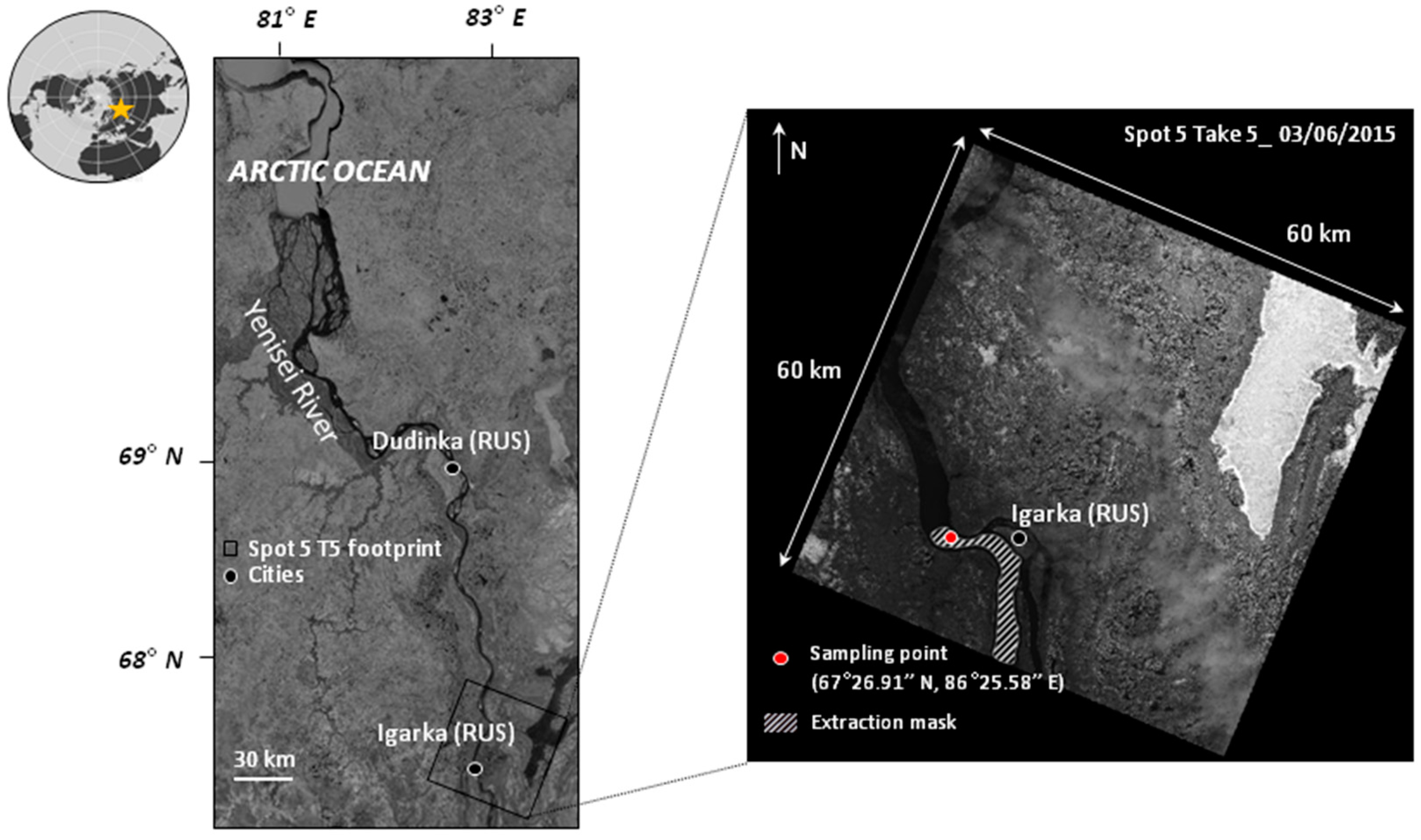
2.1. Study Site
2.2. Sample Collection and Treatment
2.3. Extraction of Water-Leaving Reflectance
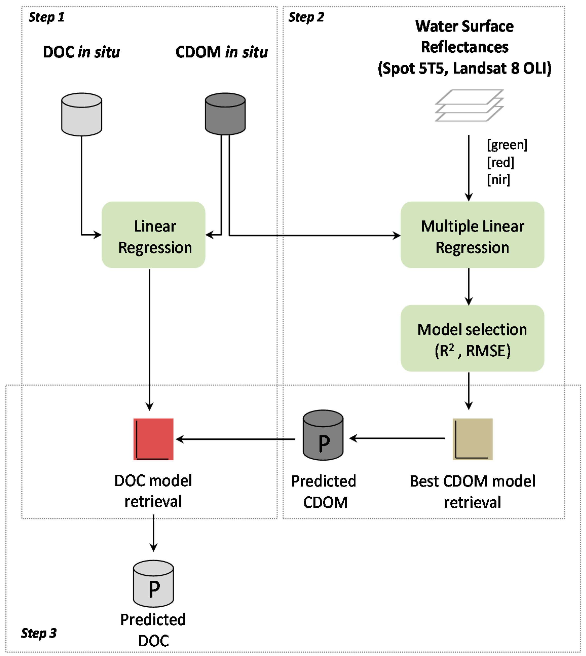
2.4. CDOM Algorithm Development
2.5. Statistical Analyses
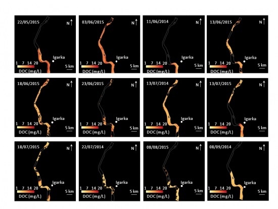
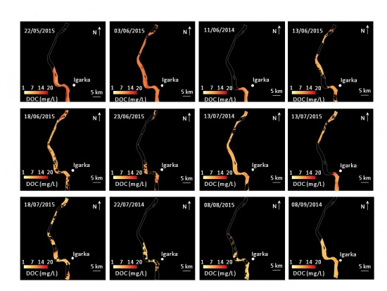
2.6. Maps Production
3. Results
4. Discussion
4.1. CDOM and DOC Estimation in Arctic Rivers
4.2. Spectral Band Configuration and CDOM Algorithms in Arctic Rivers
4.3. High Spatio-Temporal Resolution Remote Sensing Data and CDOM in Arctic Rivers
5. Conclusions
Acknowledgments
Author Contributions
Conflicts of Interest
References
- Solomon, S.; Qin, D.; Manning, M.; Chen, Z.; Marquis, M.; Averyt, K.B.; Tignor, M.; Miller, H.L. 5th Assessment Report-Climate Change 2013-IPCC; Cambridge University Press: Cambridge, UK, 2013. [Google Scholar]
- Brown, R.; Derksen, C.; Wang, L. A multi-data set analysis of variability and change in Arctic spring snow cover extent, 1967–2008. J. Geophys. Res. Atmos. 2010, 115, D16111. [Google Scholar] [CrossRef]
- Romanovsky, V.E.; Smith, S.L.; Christiansen, H.H. Permafrost thermal state in the polar Northern Hemisphere during the international polar year 2007–2009: A synthesis. Permafr. Periglac. Process. 2010, 21, 106–116. [Google Scholar] [CrossRef]
- Vonk, J.E.; Tank, S.E.; Bowden, W.B.; Laurion, I.; Vincent, W.F.; Alekseychik, P.; Amyot, M.; Billett, M.; Canario, J.; Cory, R.M. Reviews and syntheses: Effects of permafrost thaw on Arctic aquatic ecosystems. Biogeosciences 2015, 12, 7129–7167. [Google Scholar] [CrossRef]
- Lawrence, D.M.; Slater, A.G. A projection of severe near-surface permafrost degradation during the 21st century. Geophys. Res. Lett. 2005, 32, L24401. [Google Scholar] [CrossRef]
- Tarnocai, C.; Canadell, J.G.; Schuur, E.A.G.; Kuhry, P.; Mazhitova, G.; Zimov, S. Soil organic carbon pools in the northern circumpolar permafrost region. Glob. Biogeochem. Cycles 2009, 23, B003327. [Google Scholar] [CrossRef]
- Lemke, P.; Ren, J.; Alley, R.B.; Allison, I.; Carrasco, J.; Flato, G.; Fujii, Y.; Kaser, G.; Mote, P.; Thomas, R.H.; et al. Observations: Changes in snow, ice and frozen ground. In Climate Change 2007: The Physical Science Basis. Contribution of Working Group I to the Fourth Assessment Report of the Intergovernmental Panel on Climate Change; Solomon, S., Qin, D., Manning, M., Chen, Z., Marquis, M., Averyt, K.B., Tignor, M., Miller, H.L., Eds.; Cambridge University Press: Cambridge, UK, 2013. [Google Scholar]
- Zhang, J.; Lindsay, R.; Steele, M.; Schweiger, A. What drove the dramatic retreat of arctic sea ice during summer 2007? Geophys. Res. Lett. 2008, 35, L01505. [Google Scholar] [CrossRef]
- Striegl, R.G.; Aiken, G.R.; Dornblaser, M.M.; Raymond, P.A.; Wickland, K.P. A decrease in discharge-normalized DOC export by the Yukon River during summer through autumn. Geophys. Res. Lett. 2005, 32, L024413. [Google Scholar] [CrossRef]
- Prokushkin, A.S.; Pokrovsky, O.S.; Shirokova, L.S.; Korets, M.A.; Viers, J.; Prokushkin, S.G. Export of dissolved carbon from watersheds of the Central Siberian Plateau. Dock. Earth Sc. 2011, 441, 1568–1571. [Google Scholar] [CrossRef]
- Abbott, B.W.; Jones, J.B.; Schuur, E.A.G.; Chapin, F.S., III; Bowden, W.B.; Bret-Harte, M.S.; Howard, E.; Epstein, M.D.F.; Harms, T.K.; Hollingsworth, T.N.; et al. Biomass offsets little or none of permafrost carbon release from soils, streams, and wildfire: An expert assessment. Environ. Res. Lett. 2016, 11, 034014. [Google Scholar] [CrossRef]
- Kohler, H.; Meon, B.; Gordeev, V.V.; Spitzy, A.; Amon, R.M.W. Dissolved Organic Matter (DOM) in the estuaries of Ob and Yenisei and the adjacent Kara Sea, Russia. In Siberian River Run-off in the Kara Sea: Characterisation, Quantification; Stein, R., Fahl, K., Futterer, D.K., Galimov, E.M., Stepanets, O.V., Eds.; Elsevier Science: Amsterdam, The Netherlands, 2003; pp. 281–308. [Google Scholar]
- Holmes, R.M.; McClelland, J.W.; Peterson, B.J.; Tank, S.E.; Bulygina, E.; Eglinton, T.I.; Gordeev, V.V.; Gurtovaya, T.Y.; Raymond, P.A.; Repeta, D.J. Seasonal and annual fluxes of nutrients and organic matter from large rivers to the Arctic Ocean and surrounding seas. Estuar. Coasts 2012, 35, 369–382. [Google Scholar] [CrossRef]
- Amon, R.M.W.; Rinehart, A.J.; Duan, S.; Louchouarn, P.; Prokushkin, A.; Guggenberger, G.; Bauch, D.; Stedmon, C.; Raymond, P.A.; Holmes, R.M. Dissolved organic matter sources in large Arctic rivers. Geochim. Cosmochim. Acta 2012, 94, 217–237. [Google Scholar] [CrossRef] [Green Version]
- Del Castillo, C.E.; Miller, R.L. On the use of ocean color remote sensing to measure the transport of dissolved organic carbon by the Mississippi River Plume. Remote Sens. Environ. 2008, 12, 836–844. [Google Scholar] [CrossRef]
- Matsuoka, A.; Babin, M.; Doxaran, D.; Hooker, S.B.; Mitchell, B.G.; Bélanger, S.; Bricaud, A. A synthesis of light absorption properties of the Arctic Ocean: Application to semi-analytical estimates of dissolved organic carbon concentrations from space. Biogeosciences 2014, 11, 3131–3147. [Google Scholar] [CrossRef] [Green Version]
- Strömbeck, N.; Pierson, D.C. The effects of variability in the inherent optical properties on estimations of chlorophyll a by remote sensing in Swedish freshwaters. Sci. Total Environ. 2001, 268, 123–137. [Google Scholar] [CrossRef]
- Brezonik, P.; Menken, K.D.; Bauer, M. Landsat-based remote sensing of lake water quality characteristics, including chlorophyll and colored dissolved organic matter (CDOM). Lake Reserv. Manag. 2005, 21, 373–382. [Google Scholar] [CrossRef]
- Kutser, T.; Pierson, D.C.; Kallio, K.Y.; Reinart, A.; Sobek, S. Mapping lake CDOM by satellite remote sensing. Remote Sens. Environ. 2005, 94, 535–540. [Google Scholar] [CrossRef]
- Ylöstalo, P.; Kallio, K.; Seppälä, J. Absorption properties of in-water constituents and their variation among various lake types in the boreal region. Remote Sens. Environ. 2014, 148, 190–205. [Google Scholar] [CrossRef]
- Zhu, W.; Yu, Q.; Tian, Y.Q.; Chen, R.F.; Gardner, G.B. Estimation of chromophoric dissolved organic matter in the Mississippi and Atchafalaya river plume regions using above-surface hyperspectral remote sensing. J. Geophys. Res. 2011, 116, C02011. [Google Scholar] [CrossRef]
- Tian, Y.Q.; Yu, Q.; Zhu, W. Estimating of Chromophoric Dissolved Organic Matter (CDOM) with in-situ and satellite hyperspectral remote sensing technology. In Proceedings of the Geoscience and Remote Sensing Symposium (IGARSS), Munich, Germany, 22–27 July 2012.
- Brezonik, P.L.; Olmanson, L.G.; Finlay, J.C.; Bauer, M.E. Factors affecting the measurement of CDOM by remote sensing of optically complex inland waters. Remote Sens. Environ. 2015, 157, 199–215. [Google Scholar] [CrossRef]
- Fichot, C.G.; Kaiser, K.; Hooker, S.B.; Amon, R.M.; Babin, M.; Bélanger, S.; Walker, S.A.; Benner, R. Pan-Arctic distributions of continental runoff in the Arctic Ocean. Sci. Rep. 2013, 3, 1053. [Google Scholar] [CrossRef] [PubMed]
- Griffin, C.G.; Frey, K.E.; Rogan, J.; Holmes, R.M. Spatial and interannual variability of dissolved organic matter in the Kolyma River, East Siberia, observed using satellite imagery. J. Geophys. Res. 2011, 116. [Google Scholar] [CrossRef]
- Mann, P.J.; Spencer, R.G.M.; Hernes, P.J.; Six, J.; Aiken, G.R.; Tank, S.E.; McClelland, J.W.; Butler, K.D.; Dyda, R.Y.; Holmes, R.M. Pan-Arctic trends in terrestrial dissolved organic matter from optical measurements. Front. Earth Sci. 2016, 4, 25–30. [Google Scholar] [CrossRef]
- Matthews, M.W. A current review of empirical procedures of remote sensing in inland and near-coastal transitional waters. Int. J. Remote Sens. 2011, 32, 6855–6899. [Google Scholar] [CrossRef]
- Zhu, W.; Yu, Q.; Tian, Y.Q.; Becker, B.L.; Zheng, T.; Carrick, H.J. An assessment of remote sensing algorithms for colored dissolved organic matter in complex freshwater environments. Remote Sens. Environ. 2014, 140, 766–778. [Google Scholar] [CrossRef]
- Mannino, A.; Russ, M.E.; Hooker, S.B. Algorithm development and validation for satellite-derived distributions of DOC and CDOM in the US Middle Atlantic Bight. J. Geophys. Res. Oceans 2008, 113, C07051. [Google Scholar] [CrossRef]
- Lee, Z.; Carder, K.; Arnone, R.; He, M. Determination of primary spectral bands for remote sensing of aquatic environments. Sensors 2007, 7, 3428–3441. [Google Scholar] [CrossRef]
- Brando, V.E.; Dekker, A.G. Satellite hyperspectral remote sensing for estimating estuarine and coastal water quality. IEEE Trans. Geosci. Remote Sens. 2003, 41, 1378–1387. [Google Scholar] [CrossRef]
- Wang, P.; Boss, E.S.; Roesler, C. Uncertainties of inherent optical properties obtained from semi-analytical inversions of ocean color. Appl. Opt. 2005, 44, 4074–4085. [Google Scholar] [CrossRef] [PubMed]
- Carder, K.L.; Chen, F.R.; Lee, Z.P.; Hawes, S.K.; Kamykowski, D. Semianalytic moderate-resolution imaging spectrometer algorithms for chlorophyll a and absorption with bio-optical domains based on nitrate-depletion temperatures. J. Geophys. Res. Oceans 1999, 104, 5403–5421. [Google Scholar] [CrossRef]
- D’Sa, E.J.; Miller, R.L. Bio-optical properties in waters influenced by the Mississippi River during low flow conditions. Remote Sens. Environ. 2003, 84, 538–549. [Google Scholar] [CrossRef]
- Fitzmaurice, G. The meaning and interpretation of interaction. Nutrition 2000, 16, 313–314. [Google Scholar] [CrossRef]
- Martinez, J.-M.; Guyot, J.-L.; Filizola, N.; Sondag, F. Increase in suspended sediment discharge of the Amazon River assessed by monitoring network and satellite data. Catena 2009, 79, 257–264. [Google Scholar] [CrossRef]
- Nunes, A.L.; Marçal, A.R.S. Atmospheric correction of high resolution multi-spectral satellite images using a simplified method based on the 6S Code. In Proceedings of the 4th Remote Sensing and Photogrammetry Society Annual Conference-Mapping and Resources Management, Aberdeen, Scotland, 16–18 May 2000.
- Hoge, F.E.; Lyon, P.E. Satellite observation of Chromophoric Dissolved Organic Matter (CDOM) variability in the wake of hurricanes and typhoons. Geophys. Res. Lett. 2002, 29, 141–144. [Google Scholar] [CrossRef]
- Shiklomanov, I.A.; Shiklomanov, A.I.; Lammers, R.B.; Peterson, B.J.; Vorosmarty, C.J. The dynamics of river water inflow to the Arctic Ocean. In The Freshwater Budget of the Arctic Ocean; Springer: Dordrecht, The Netherlands, 2000; pp. 281–296. [Google Scholar]
- Yang, D.; Ye, B.; Kane, D.L. Streamflow changes over Siberian Yenisei River basin. J. Hydrol. 2004, 296, 59–80. [Google Scholar] [CrossRef]
- Serreze, M.C.; Bromwich, D.H.; Clark, M.P.; Etringer, A.J.; Zhang, T.; Lammers, R. Large-scale hydro-climatology of the terrestrial Arctic drainage system. J. Geophys. Res. 2002, 108. [Google Scholar] [CrossRef]
- Stuefer, S.; Daqing, Y.; Shiklomanov, A. Effect of streamflow regulation on mean annual discharge variability of the Yenisei River. IAHS-AISH Publ. 2011, 346, 27–32. [Google Scholar]
- Lobbes, J.M.; Fitznar, H.P.; Kattner, G. Biogeochemical characteristics of dissolved and particulate organic matter in Russian rivers entering the Arctic Ocean. Geochim. Cosmochim. Acta 2000, 64, 2973–2983. [Google Scholar] [CrossRef]
- Dittmar, T.; Kattner, G. The biogeochemistry of the river and shelf ecosystem of the Arctic Ocean: A review. Mar. Chem. 2003, 83, 103–120. [Google Scholar] [CrossRef]
- Amon, R.M.; Meon, B. The biogeochemistry of dissolved organic matter and nutrients in two large Arctic estuaries and potential implications for our understanding of the Arctic Ocean system. Mar. Chem. 2004, 92, 311–330. [Google Scholar] [CrossRef]
- Hagolle, O.; Huc, M.; Villa Pascual, D.; Dedieu, G. A multi-temporal and multi-spectral method to estimate aerosol optical thickness over land, for the atmospheric correction of FormoSat-2, LandSat, VENμS and Sentinel-2 Images. Remote Sens. 2015, 7, 2668–2691. [Google Scholar] [CrossRef]
- USGS. L8SR Product Guide: Provisional Landsat 8 Surface Reflectance Product; (Version 2.0); USGS: Reston, VA, USA, 2015; p. 27.
- McClelland, J.W.; Holmes, R.M.; Peterson, B.J.; Amon, R.; Brabets, T.; Cooper, L.; Gibson, J.; Gordeev, V.V.; Guay, C.; Milburn, D. Development of a Pan-Arctic database for river chemistry. Eos Trans. Am. Geophys. Union 2008, 89, 217–218. [Google Scholar] [CrossRef]


| Satellite Sensor | Acquisition Date | Nearest Sampling Date of DOC |
|---|---|---|
| Landsat 8 OLI | 22 May 2015 | 22 May 2015 |
| SPOT5 HRV (Take5) | 3 June 2015 | 3 June 2015 |
| Landsat 8 OLI | 11 June 2014 | 13 June 2014 |
| SPOT5 HRV (Take5) | 13 June 2015 | 13 June 2015 |
| SPOT5 HRV (Take5) | 18 June 2015 | 18 June 2015 |
| SPOT5 HRV (Take5) | 23 June 2015 | 24 June 2015 |
| Landsat 8 OLI | 13 July 2014 | 11 July 2014 |
| SPOT5 HRV (Take5) | 13 July 2015 | 13 July 2015 |
| SPOT5 HRV (Take5) | 18 July 2015 | 18 July 2015 |
| Landsat 8 OLI | 22 July 2014 | 23 July 2014 |
| Landsat 8 OLI | 8 August 2015 | 12 August 2015 |
| Landsat 8 OLI | 8 September 2014 | 9 September 2014 |
| Explanatory Variables | Description | |
|---|---|---|
| Model (1) with green | ||
| Model form: E(y) = β0 + β1 | ||
| Green | β1 | Green band |
| Model (2) with red | ||
| Model form: E(y) = β10 + β11 | ||
| Red | β11 | Red band |
| Model (3) with green and red | ||
| Model form: E(y) = β20 + β21 + β22 | ||
| Green | β21 | Green band |
| Red | β22 | Red band |
| Model (4) with a green/red ratio | ||
| Model form: E(y) = β30 + β31 | ||
| Green/Red | β31 | Ratio term between the Green band and the Red band |
| Model (5) with an green: red interaction | ||
| Model form: E(y) = β40 + β41 | ||
| Green: Red | β41 | Interaction term between the Green band and the Red band |
| Model (6) with green and a green/red ratio | ||
| Model form: E(y) = β50 + β51 + β52 | ||
| Green | β51 | Green band |
| Green/Red | β52 | Ratio term between the Green band and the Red band |
| Model (7) with green and green: red interaction | ||
| Model form: E(y) = β60 + β61 + β62 | ||
| Green | β61 | Green |
| Green: Red | β62 | Interaction term between the Green band and the Red band |
| Sampling Date | Gap * (in Days) | DOC (mg/L) | a440 (m−1) | TSS (mg/L) | SRblue | SRgreen | SRred |
|---|---|---|---|---|---|---|---|
| 22 May 2015 | 0 | 15.58 | 10.43 | 19.90 | 0.03705 | 0.03832 | 0.01526 |
| 3 June 2015 | 0 | 10.72 | 7.23 | 17.57 | 0.01793 | 0.02628 | 0.02260 |
| 13 June 2014 | 2 | 9.63 | 7.71 | 8.32 | 0.03576 | 0.03303 | 0.01721 |
| 13 June 2015 | 0 | 9.43 | 5.76 | 17.75 | 0.01913 | 0.02260 | 0.02536 |
| 18 June 2015 | 0 | 8.00 | 3.96 | 10.97 | 0.01983 | 0.02245 | 0.03267 |
| 24 June 2015 | 1 | 8.13 | 6.17 | 11.90 | 0.02354 | 0.02982 | 0.03519 |
| 11 July 2014 | 2 | 6.78 | 4.42 | 6.73 | 0.01761 | 0.01724 | 0.01489 |
| 13 July 2015 | 0 | 7.11 | 3.43 | 3.23 | 0.02418 | 0.02586 | 0.03697 |
| 18 July 2015 | 0 | 8.47 | 2.24 | - | 0.02337 | 0.02199 | 0.03054 |
| 23 July 2014 | 1 | 5.03 | 2.72 | 2.63 | 0.02258 | 0.01857 | 0.01504 |
| 12 August 2015 | 4 | 4.53 | 1.27 | 3.50 | 0.03096 | 0.02352 | 0.01782 |
| 9 September 2014 | 1 | 6.26 | 3.87 | 6.17 | 0.01929 | 0.01739 | 0.00640 |
| Model | Dataset | Explanatory Variables | Estimates | p-Value | R2 | RMSE |
|---|---|---|---|---|---|---|
| Model (1) | Yenisei | Intercept | 3.703 | n.s | 0.02 | 2.47 |
| Green | 50.7 | n.s | ||||
| Model (2) | Yenisei | Intercept | 0.917 | n.s | 0.22 | 2.20 |
| Red | 160.58 | n.s | ||||
| Model (3) | Yenisei | Intercept | 0.8719 | n.s | 0.44 | 1.86 |
| Green | −269.2196 | |||||
| Red | 423.4267 | * | ||||
| Model (4) | Yenisei | Intercept | 11.022 | ** | 0.25 | 2.17 |
| Green/Red | −6.308 | n.s | ||||
| Model (5) | Yenisei | Intercept | 3.105 | * | 0.19 | 2.25 |
| Green: Red | 2764.630 | n.s | ||||
| Model (6) | Yenisei | Intercept | 10.819 | ** | 0.54 | 1.68 |
| Green | 195.221 | * | ||||
| Green/Red | −11.004 | * | ||||
| Model (7) | Yenisei | Intercept | 10.606 | *** | 0.76 | 1.21 |
| Green | −681.477 | ** | ||||
| Green: Red | 16410.925 | *** | ||||
| Model (8) | Kolyma 1 | Intercept | 5.823 | *** | 0.41 | 3.24 |
| Green | −128.390 | * | ||||
| Green: Red | 1602.988 | * |
© 2016 by the authors; licensee MDPI, Basel, Switzerland. This article is an open access article distributed under the terms and conditions of the Creative Commons Attribution (CC-BY) license (http://creativecommons.org/licenses/by/4.0/).
Share and Cite
Herrault, P.-A.; Gandois, L.; Gascoin, S.; Tananaev, N.; Le Dantec, T.; Teisserenc, R. Using High Spatio-Temporal Optical Remote Sensing to Monitor Dissolved Organic Carbon in the Arctic River Yenisei. Remote Sens. 2016, 8, 803. https://doi.org/10.3390/rs8100803
Herrault P-A, Gandois L, Gascoin S, Tananaev N, Le Dantec T, Teisserenc R. Using High Spatio-Temporal Optical Remote Sensing to Monitor Dissolved Organic Carbon in the Arctic River Yenisei. Remote Sensing. 2016; 8(10):803. https://doi.org/10.3390/rs8100803
Chicago/Turabian StyleHerrault, Pierre-Alexis, Laure Gandois, Simon Gascoin, Nikita Tananaev, Théo Le Dantec, and Roman Teisserenc. 2016. "Using High Spatio-Temporal Optical Remote Sensing to Monitor Dissolved Organic Carbon in the Arctic River Yenisei" Remote Sensing 8, no. 10: 803. https://doi.org/10.3390/rs8100803