Satellite Remote Sensing in Seismology. A Review

Scientific Research Centre for Ecological Safety, Russian Academy of Sciences, 18, Korpusnaya st., St-Petersburg, 197110, Russia
Remote Sens. 2010, 2(1), 124-150; https://doi.org/10.3390/rs2010124
Submission received: 15 October 2009
/
Revised: 18 December 2009
/
Accepted: 23 December 2009
/
Published: 30 December 2009
(This article belongs to the Special Issue Remote Sensing in Seismology)
Abstract
:A wide range of satellite methods is applied now in seismology. The first applications of satellite data for earthquake exploration were initiated in the ‘70s, when active faults were mapped on satellite images. It was a pure and simple extrapolation of airphoto geological interpretation methods into space. The modern embodiment of this method is alignment analysis. Time series of alignments on the Earth's surface are investigated before and after the earthquake. A further application of satellite data in seismology is related with geophysical methods. Electromagnetic methods have about the same long history of application for seismology. Stable statistical estimations of ionosphere-lithosphere relation were obtained based on satellite ionozonds. The most successful current project "DEMETER" shows impressive results. Satellite thermal infra-red data were applied for earthquake research in the next step. Numerous results have confirmed previous observations of thermal anomalies on the Earth's surface prior to earthquakes. A modern trend is the application of the outgoing long-wave radiation for earthquake research. In ‘80s a new technology—satellite radar interferometry—opened a new page. Spectacular pictures of co-seismic deformations were presented. Current researches are moving in the direction of pre-earthquake deformation detection. GPS technology is also widely used in seismology both for ionosphere sounding and for ground movement detection. Satellite gravimetry has demonstrated its first very impressive results on the example of the catastrophic Indonesian earthquake in 2004. Relatively new applications of remote sensing for seismology as atmospheric sounding, gas observations, and cloud analysis are considered as possible candidates for applications.
1. Introduction
Remote sensing has been used for earthquake research from the ‘70s, with the first appearance of satellite images. First of all it was used in structural geological and geomorphological research. Active faults and structures were mapped on the base of satellite images. This method is very limited in time series analysis. There was no possibility to measure short term processes before and after the earthquake. It was simple an extrapolation of airphoto geological interpretation methods into space. The modern version of this method is active tectonic analysis with the application of alignment analysis. Time series of alignment distributions on the Earth's surface are investigated before and after an earthquake.
The current situation of remote sensing application for earthquake research indicates a few phenomena, related with earthquakes, particularly the Earth's surface deformation, surface temperature and humidity, atmosphere temperature and humidity, gas and aerosol content. Both horizontal and vertical deformations scaled from tens of centimeters to meters are recorded after the shock. Such deformations are recorded by the Interferometric Synthetic Aperture Radar (InSAR) technique with confidence. Pre-earthquake deformations are rather small, on the order of centimeters. A few cases of deformation mapping before the shock using satellite data are known at present time. Future developments lay in precision longwave SAR systems with medium spatial resolution and combined with the GPS technique. There are numerous observations of surface and near surface temperature increases of 3–5 °C prior to Earth crust earthquakes. Methods of earthquake prediction are developing using thermal infrared (TIR) surveys. Multiple evidence of gas and aerosol content changes before earthquakes are reported for ground observations. Satellite methods allow one to measure the concentrations of gases in atmosphere: O3, CH4, CO2, CO, H2S, SO2, HCl and aerosols. However the spatial resolution and sensitivity of modern systems restricts the application of satellite gas observation in seismology and the first promising results have been obtained only for ozone, aerosol and air humidity.
A few reviews have covered the field of satellite data applications for natural hazards [1,2,3,4]. Only some of them were concentrated on earthquake research [5,6,7]. A special issue of the Journal of Asian Earth Sciences entitled “Validation of Earthquake Precursors (by Satellite, Terrestrial and other Observations)-VESTO” will be published at the near future.
2. Deformations
One of the main directions of remote sensing application for seismology is deformation mapping. Surface deformations in seismic cycles can be divided into three phases: pre-seismic or inter-seismic, co-seismic and post-seismic ones. Co-seismic deformations are evaluated up to meters and tens of meters while pre-seismic movements amount to centimeters. Post-seismic deformations are also measured in centimeters, but subsequent landslides can increase deformations to meters. Most current research is focused on co-seismic and post-seismic (landslide) deformations.
2.1. Optical Sensors
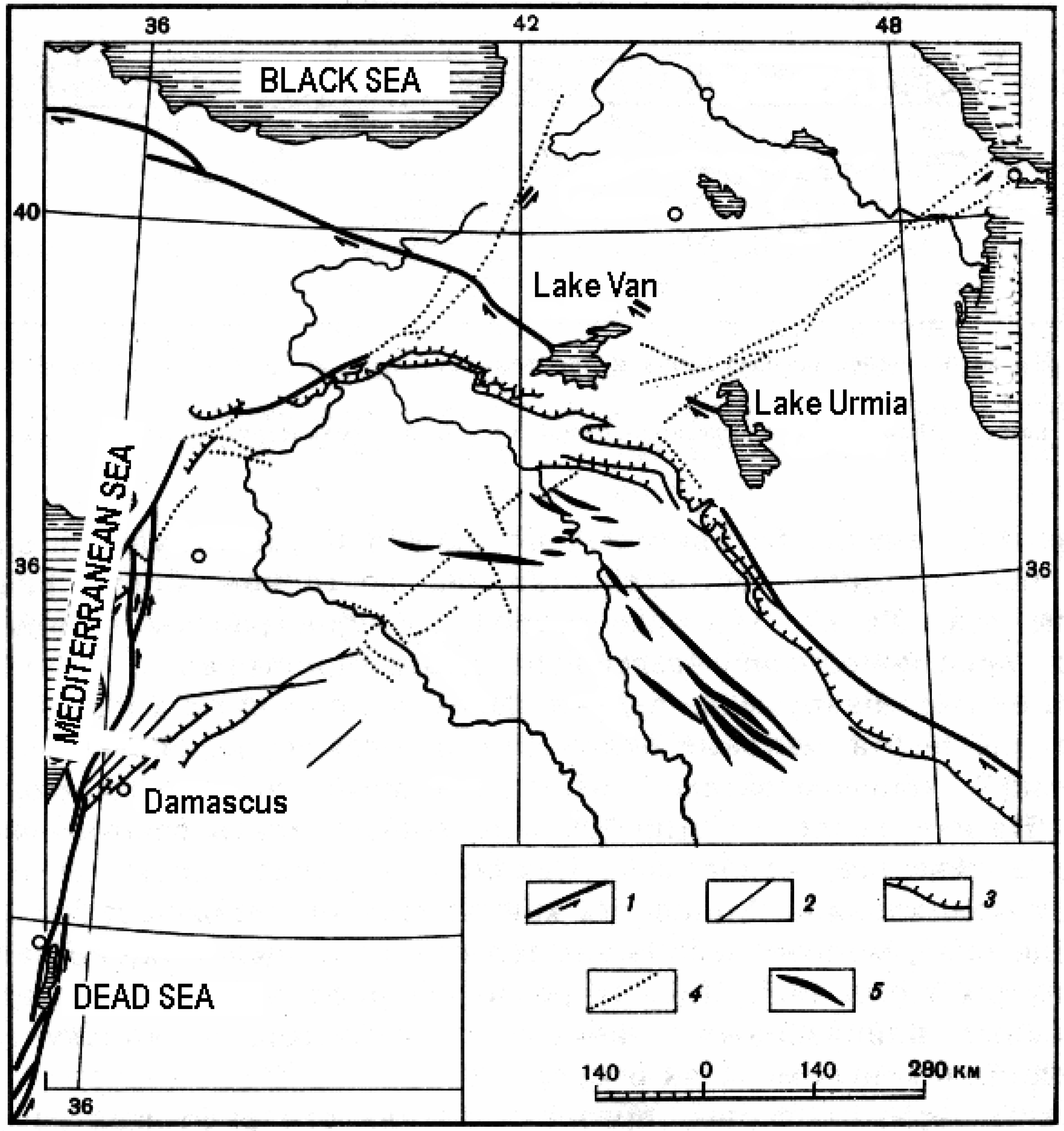
The first application of satellite images in seismology was related to structural geology and geomorphology. Active faults and neotectonics were the research aims [8,9]. Epicenter zones of recent earthquakes were studied on the space images. Image interpretation depended on visual methods. The interpreter selected faults with sharp borders, shift of river valleys, etc. One example of such an application is shown on Figure 1.
Figure 1.
Main fault systems of North Arabian plate [10]:1―active faults; 2―late Cenozoic faults; 3―Cenozoic thrusts; 4―alignment on the base of satellite images; 5―anticlines.
Figure 1.
Main fault systems of North Arabian plate [10]:1―active faults; 2―late Cenozoic faults; 3―Cenozoic thrusts; 4―alignment on the base of satellite images; 5―anticlines.

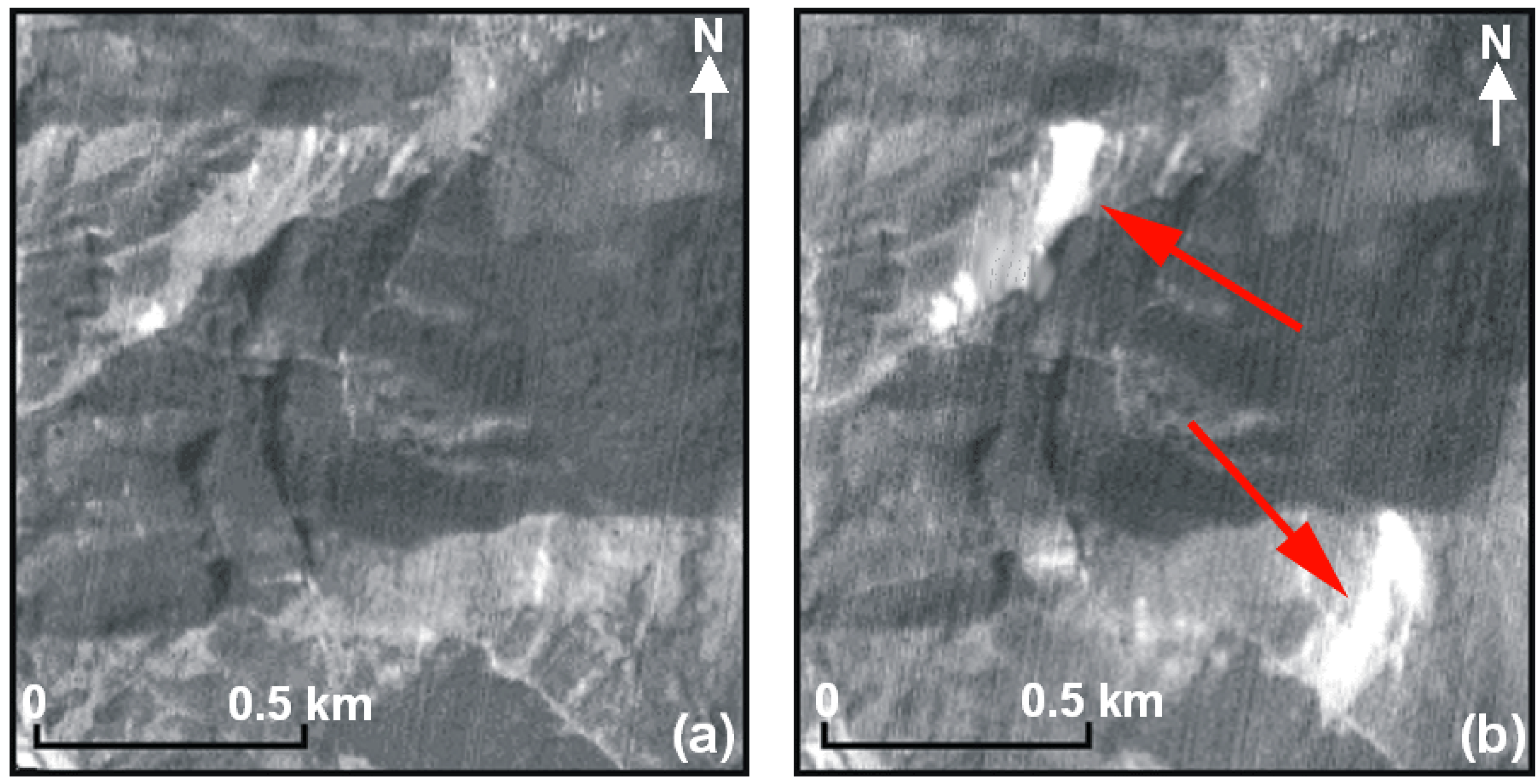
Co-seismic and post-seismic (landslides) deformations are mapped by modern optic satellite systems. Typical example of high resolution satellite images application for surface deformation is presented on Figure 2. Change detection methods are widely used for landslide deformation mapping.
Figure 2.
Surface deformations mapping for the Chamoli earthquake (M = 6.3, 29 March 1999 Himalaya, India). Change detection after the earthquake [11]. (a) IRS-1C-PAN pre-earthquake image of 26 March 1999. (b) IRS-1C-PAN post-earthquake image of 31 March 1999.
Figure 2.
Surface deformations mapping for the Chamoli earthquake (M = 6.3, 29 March 1999 Himalaya, India). Change detection after the earthquake [11]. (a) IRS-1C-PAN pre-earthquake image of 26 March 1999. (b) IRS-1C-PAN post-earthquake image of 31 March 1999.
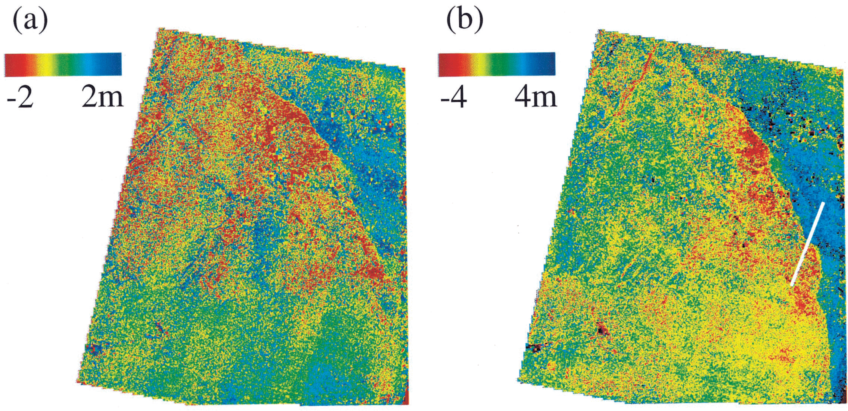
Deformation mapping with optical systems as a technique to measure horizontal movements was developed recently, after the InSAR deformation method (see Section 2.2). The technique is based on a sub-pixel correlation technique [12]. Mis-registration due to stereoscopic effects is compensated together with those due to the changing attitude of the satellite during image acquisition. Residual mis-registrations then reflect ground deformation. SPOT panchromatic images were applied to the Landers earthquake, 1992, USA [12]; the Izmit earthquake, 1999, Turkey [13], and the Chi-chi earthquake, 1999, in Taiwan [14]. The technique provides measurements with an accuracy of about 0.5 m. The displacement field obtained from this technique can be used to map co-seismic ground deformations and measure slips on the fault. InSAR technique provides precise measurements a few kilometers away from the faults but usually can not generate complete deformation map in the near-fault zone. Optical displacement method can supplement InSAR technique to cover this disadvantage of the InSAR technique.
Lineament analysis has become the new step in the application of optical data sensors in seismology. Time series of alignment distributions on the Earth's surface are investigated before and after an earthquake. Significant changes in alignment distributions (density, direction) were recorded before an earthquake [15].
The application of optical methods for deformation mapping has limited use now due to cloud problems. It does not allow one to get long time image series for analysis. On the other hand, the physical basis of optical sensor applications for deformation mapping before the shock are not clear. The main trend of optical sensors in the nearest future will be related with post-seismic deformation mapping, especially in epicenter areas, with high resolution satellite systems.
Figure 3.
Horizontal ground displacement induced by the Landers earthquake measured from SPOT2 panchromatic images (pixel size 10 m). (a) East-West. (b) North-South components [12].
Figure 3.
Horizontal ground displacement induced by the Landers earthquake measured from SPOT2 panchromatic images (pixel size 10 m). (a) East-West. (b) North-South components [12].

2.2. InSAR
The InSAR technique is used to examine small-scale features in the deformation field associated with earthquakes. Satellite interferometry is based on multitemporal radar observations. InSAR is a method by which the phase differences of two or more SAR images are used to calculate the differences in range from two SAR antennae having slightly different viewing geometries to targets on the ground. As a result, displacements on the Earth's surface in range of centimeters and millimeters can be measured. The InSAR results show significant deformation signatures associated with faults, fractures and subsidences. The interferogram also clearly indicates surface deformation related to earthquakes.
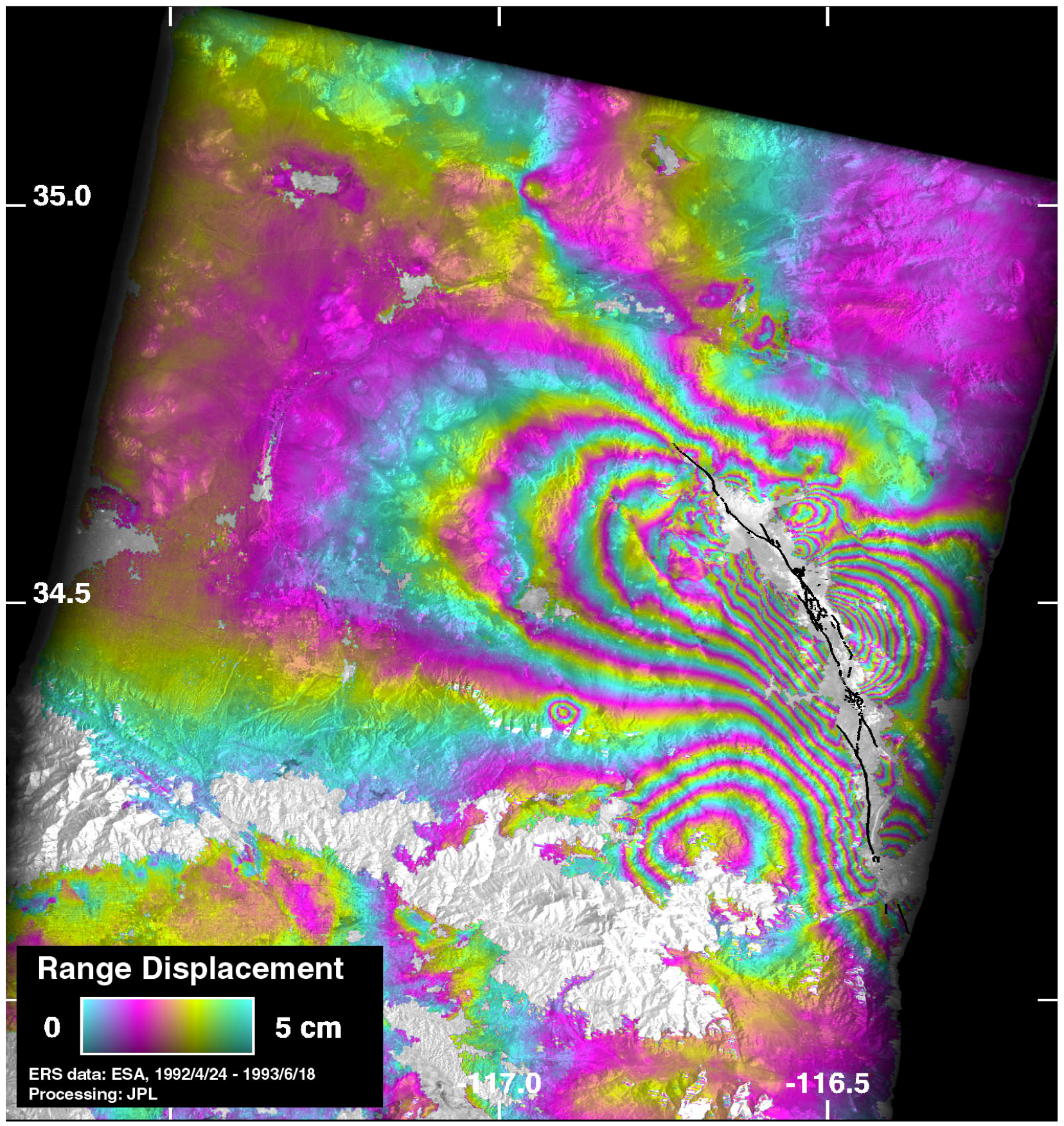
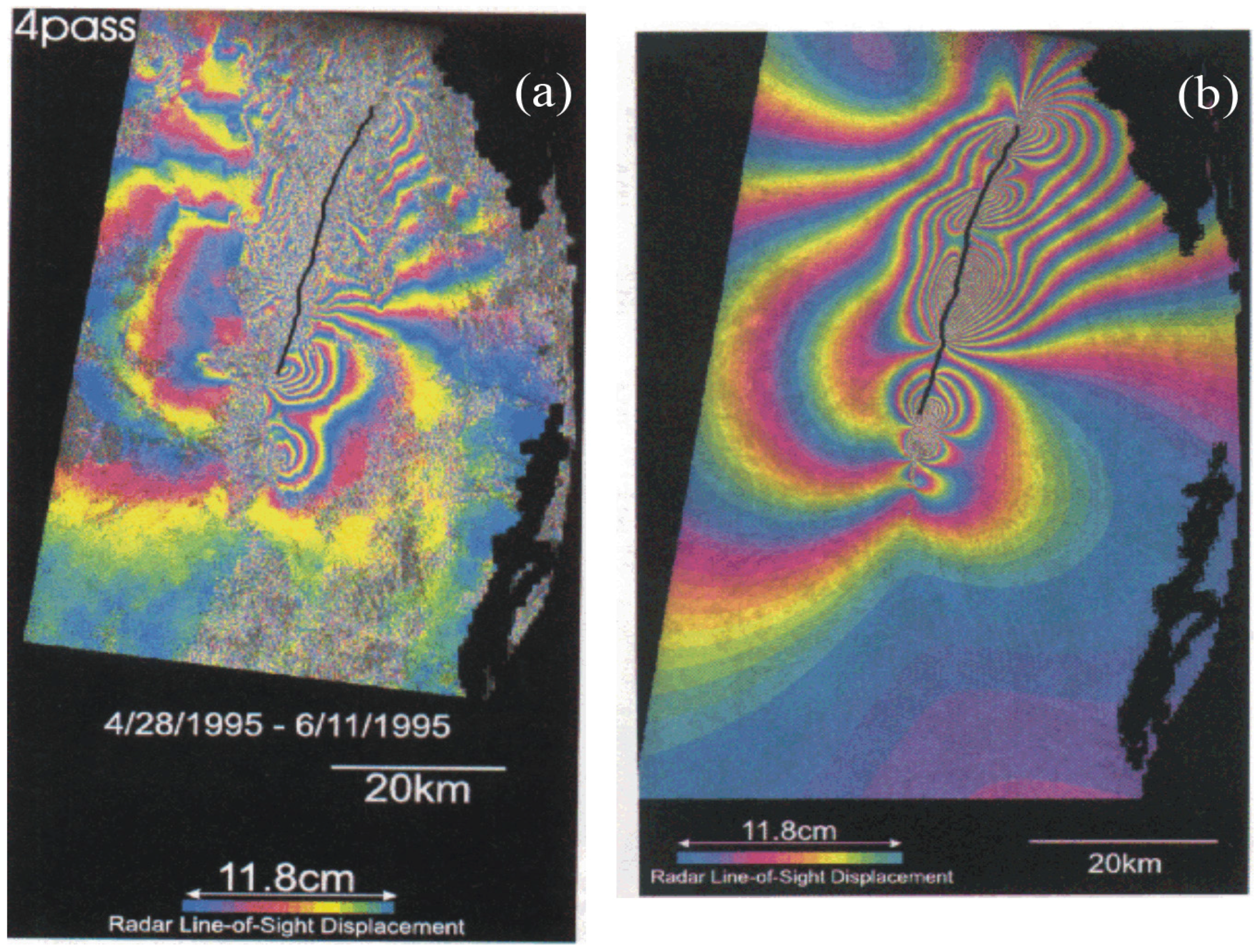
The first application of satellite interferometry for earthquake research was demonstrated in the ‘90s by Massonnet et al. [16]. The well-known “butterfly” image (Figure 4) of the Landers earthquake (M = 7.3, 28 June 1992) was compiled on the base of pre-seismic image of April 24, 1992 and post-seismic scenes: August 7, 1992; 3 July, 1992 and June 18, 1993 [17]. The comparison of the observed interferometric picture and modeled scheme of earthquake deformations shows many similar details (Figure 5). Similar images have been obtained for all the significant earthquakes of the last decade: Neftegorsk, 1995, Russia [18], Bhuj, 2001, India [19]; Bam, 2003, Iran [20]; Sumatra (2004), Indonesia [21] etc. All these cases demonstrate co-seismic and post-seismic deformations.
Figure 4.
Observed co-seismic interferogram for the Landers earthquake (M = 7.3, 28 June 1992, CA, USA). One full color cycle represents here 5 cm of range displacement. Solid lines depict the fault geometry as mapped in the field. Gray areas are zones of low phase coherence that have been masked before phase unwrapping [17].

Figure 5.
Ground deformations induced by the Neftegorsk earthquake (M = 7.6, 28 May 1995, Sakhalin, Russia). (a) Radar interferogram. (b) Deformation model prediction [18].
Figure 5.
Ground deformations induced by the Neftegorsk earthquake (M = 7.6, 28 May 1995, Sakhalin, Russia). (a) Radar interferogram. (b) Deformation model prediction [18].
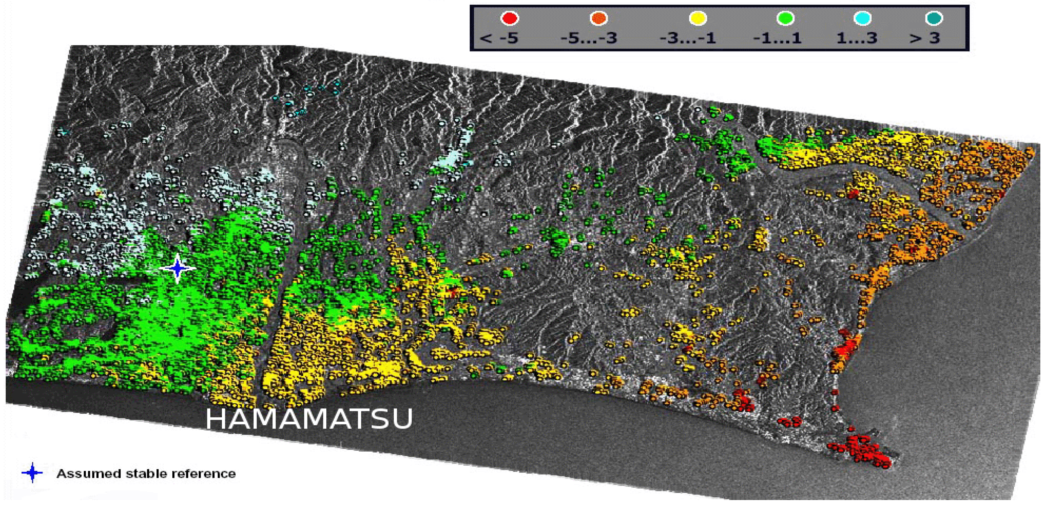
First results with pre-seismic deformations recorded with InSAR technique were obtained recently. Probable pre-seismic deformation in the Tokai region, Japan (Figure 6) is indicated [22] on the multiyear InSAR data. The Tokai region is a well-known seismic gap located about 200 km southwest of Tokyo, at the conjunction of the Eurasian plate, the Philippine sea plate and the North-American plate. The vertical deformation recorded on the base of InSAR data coincides with ground leveling and GPS observation (Figure 10). The subsidence continues to this moment, but an earthquake has still not happened.
Figure 6.
Average displacement rate in Tokai area, Japan, 1992–2000 years, vertical deformation, mm/year [22].
Figure 6.
Average displacement rate in Tokai area, Japan, 1992–2000 years, vertical deformation, mm/year [22].

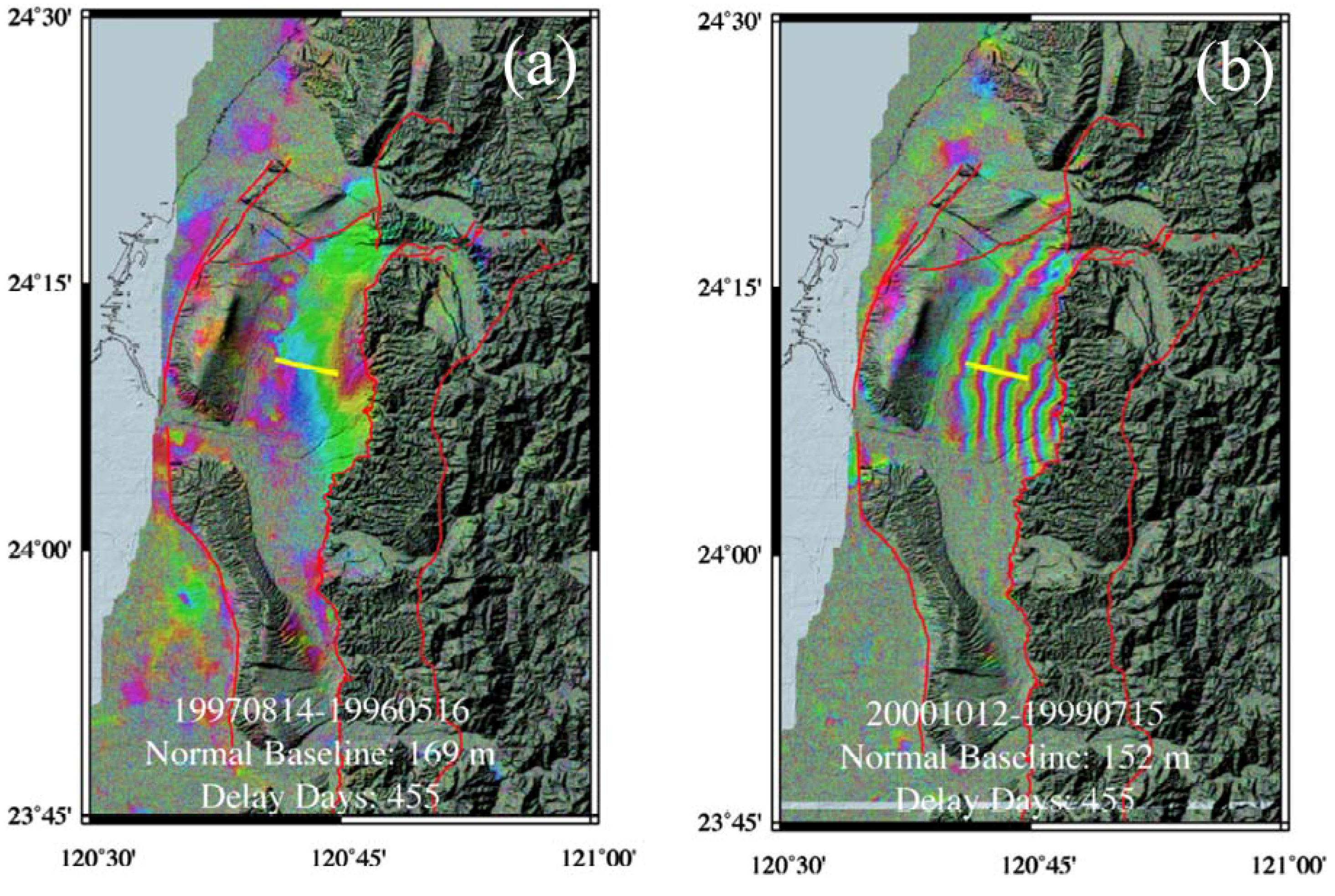
The following research has shown surface deformations three year before the Chi-chi earthquake (1999, Taiwan [23]). ERS-2 radar scenes were used to identify possible precursory surface deformation in the areas of the main fault before the Chi-Chi earthquake. It was found that surface deformation began at least three years before the Chi-Chi earthquake in the areas to the west of the northern segment of the fault where clear co-seismic surface deformation patterns were observed (Figure 7).
Figure 7.
Pre-seismic and co-seismic ground deformations for the Chi-Chi earthquake (M = 7.6, 20 September 1999, Taiwan). (a) Pre-seismic deformations between 16 May 1996 and 14 August 1997. (b) Co-seismic ground deformations between 15 July 1999 and 12 October 2000 [23].
Figure 7.
Pre-seismic and co-seismic ground deformations for the Chi-Chi earthquake (M = 7.6, 20 September 1999, Taiwan). (a) Pre-seismic deformations between 16 May 1996 and 14 August 1997. (b) Co-seismic ground deformations between 15 July 1999 and 12 October 2000 [23].
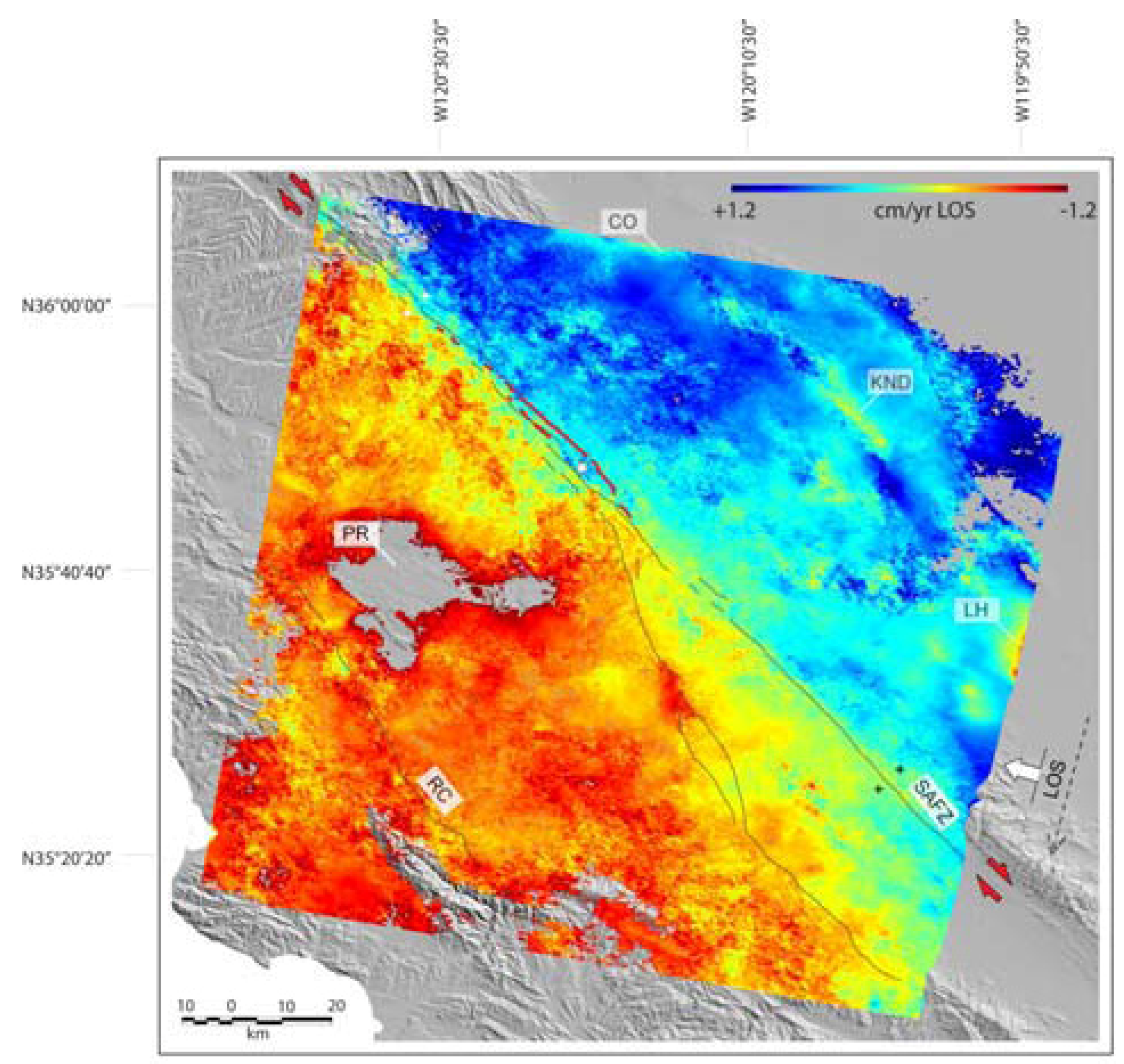
One of the other applications has described pre-seismic deformations related with the 2004 Parkfield earthquake [24]. Pre-seismic movements are clearly recorded for strike-slips like the San Andreas Fault Zone by InSAR. The relative horizontal speed of the slip is evaluated at about 2 cm/year. The spatial pattern of the pre-seismic InSAR deformation rate (Figure 8) indicates that strain distribution is not uniformly partitioned along the fault strike.
Figure 8.
Pre-seismic strain buildup on the San Andreas Fault Zone at Parkfield. The map is composed by averaging 20 unwrapped ERS-1/2 interferograms in a stack. Each 20 × 20 m pixel is then a measure of the average in the line of sight direction velocity in the period 1992–2004 prior to the earthquake. The scale-bar values represent centimeters parallel to the fault [24].

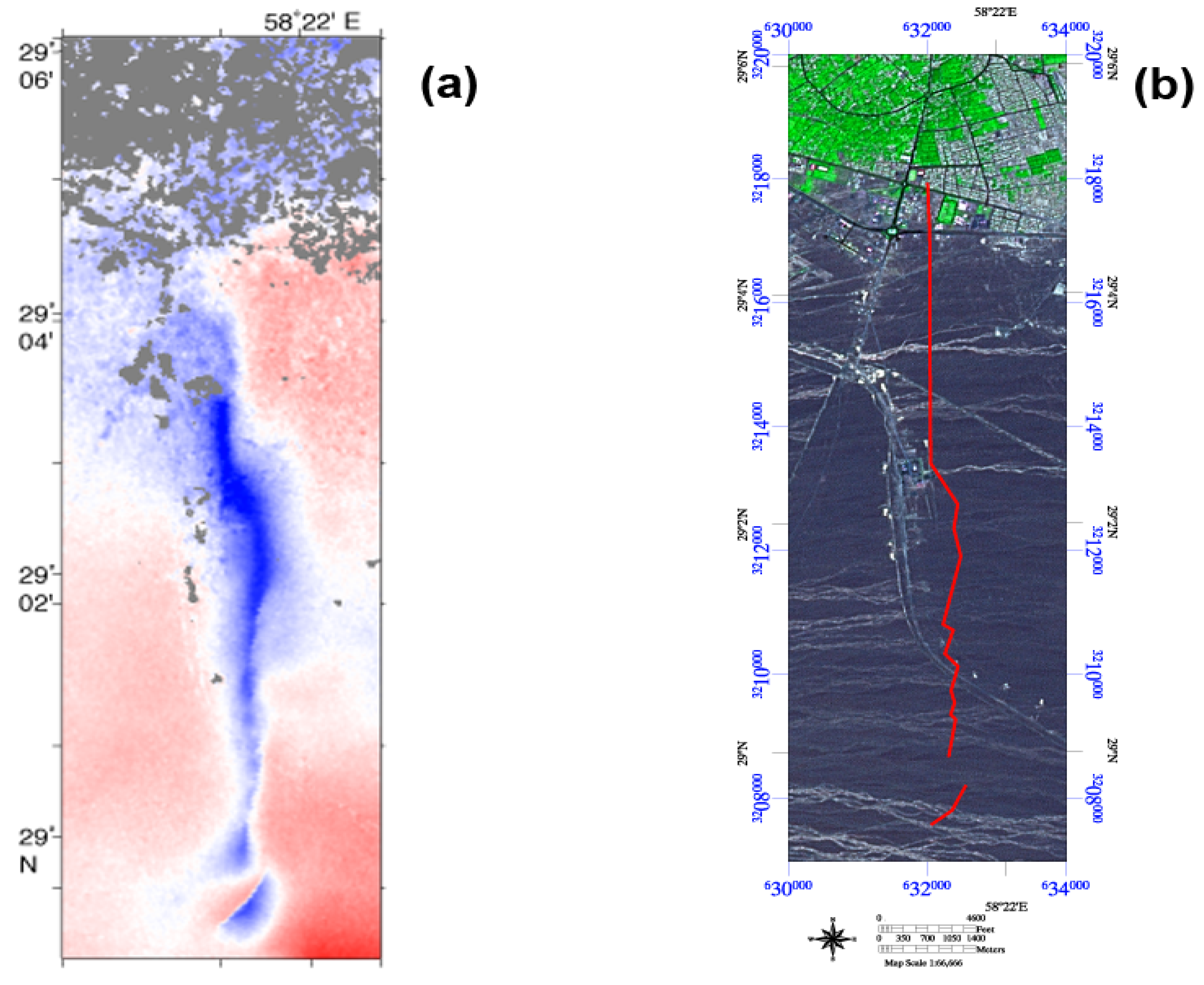
Post-seismic deformations also became the object of research. It was possible to separate co-seismic and post-seismic deformations for the Bam earthquake (Iran). A subsidence of about 3 cm was observed (Figure 9) in the area of the destructive fault three years after the main shock [25].
Figure 9.
Post-seismic deformations for the Bam earthquake (M = 6.6, 26 December 2003, Iran). (a) Vertical displacement of the land surface south of Bam, during the three and a half years after the earthquake derived from analysis of radar images. The dark blue area sank a total of more than 3 cm (1.2 inches), revealing a zone of rock that was damaged during the earthquake and then healed afterwards. (b) False-color Landsat Thematic Mapper image taken on October 1, 1999 of the area of the earthquake rupture south of Bam. Red line shows location of the fault damage zone above the buried 2003 rupture. Vegetation in the city of Bam is green and stone-covered desert has various tones of gray [25].

The further enhancement of the InSAR technology will allow us to record very fine difference in surface displacement. The currently operated COSMO/SkyMed mission aims to provide daily observations, overcoming limited observational frequency, by using a constellation of four satellites. The current constellation consists of three medium-size satellites, each one equipped with a microwave high-resolution SAR operating in X-band (31 mm), having ~600 km single side access ground area, orbiting in a sun-synchronous orbit at ~620 km height over the Earth surface, with the capability to change attitude in order to acquire images at both right and left side of the satellite ground track. TERRASAR-X (wavelength-31 mm) radar also provides reliable information for surface deformation measurements.
Existing satellite InSAR instruments have X-band and C-band (a wavelength of 56.6 mm), offering high resolution, but they only provide reliable interferograms for coherent, non-vegetated surfaces. Data from the JERS-1 satellite demonstrated during its lifetime that L-band (236 mm wavelength) satellites propose reduced resolution but provide interferograms over a far greater range of surface cover types. Modern L-band (236 mm wavelength) SAR PALSAR onboard Japanese satellite ALOS supplies high quality data for interferometry. Unfortunately, this instrument is designed to test applications other than interferometry, so it provides only limited support for deformation analysis. Future missions like MOSART (Monitoring of Surface Deformation in Active Tectonic Zones) and TERRASAR-L are still not realized.
The InSAR technique opens new fields of remote sensing applications in seismology. InSAR methods are the best tool to study earthquake deformations at the moment after the shock. New systems will allow us to shift to pre-seismic deformation measurements and earthquake forecasting. Epicenter area deformations are still problem for InSAR due to coherence loss and permanent scatter destruction.
2.3. GPS
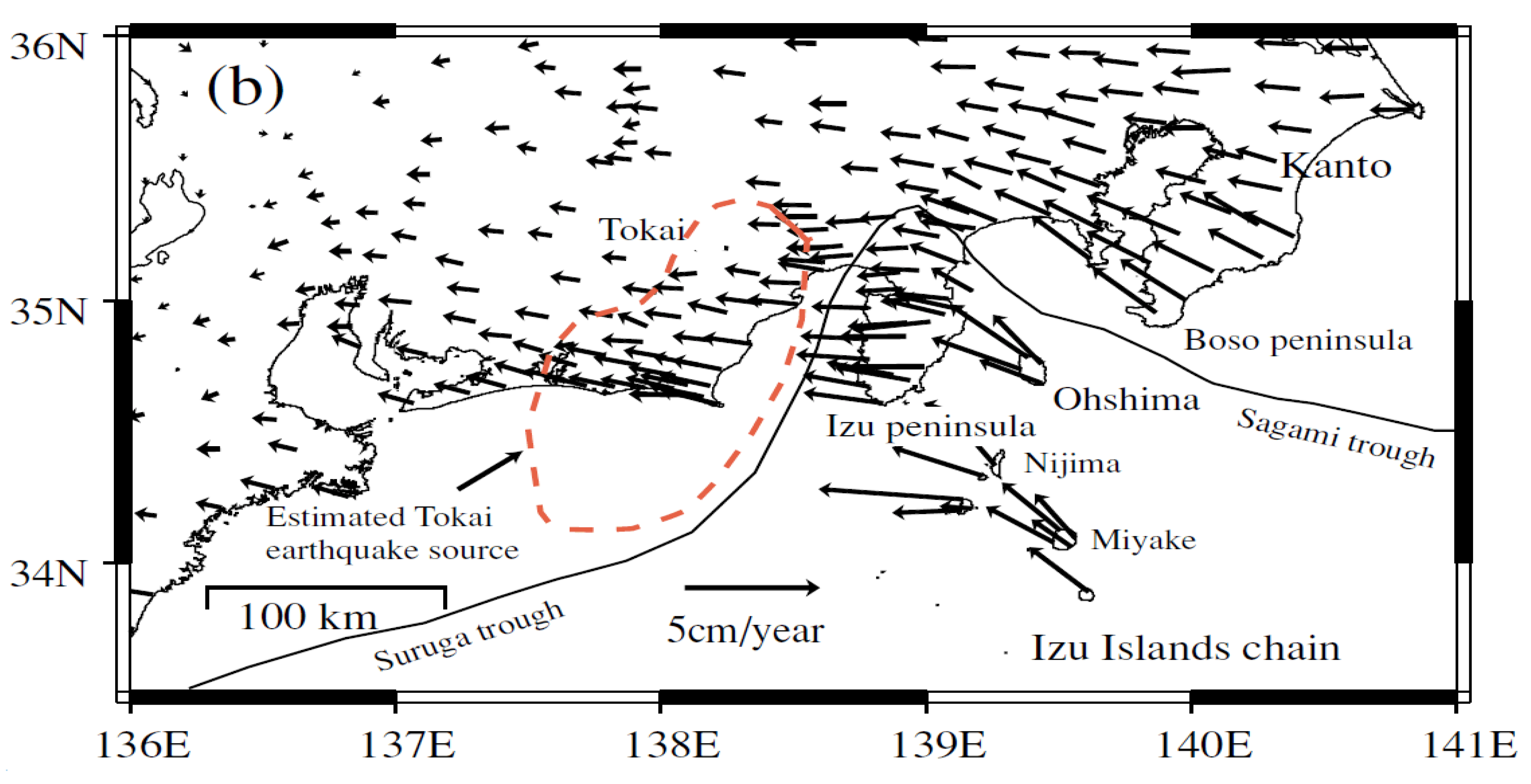
As GPS observations are not strictly a remote sensing application, only a few examples of their use for the study of surface deformations will be listed below. It was mentioned above that InSAR technique is more sensitive for vertical deformations, while the GPS method is capable of recording long period horizontal movements. Vertical ground deformations in Tokai area, Japan, revealed by InSAR (Figure 6) were accompanied by horizontal ones recorded (Figure 10) by GPS [26].
Figure 10.
Horizontal deformations in Tokai area, measured by GPS. The Philippine sea plate subducts beneath the continental plate from the Suruga and Sagami troughs. The black arrow represents the observed ground displacement rate in cm/year for the period between 1997 and 1999. Stroke line represents the estimated source area of the expected Tokai earthquake [26].

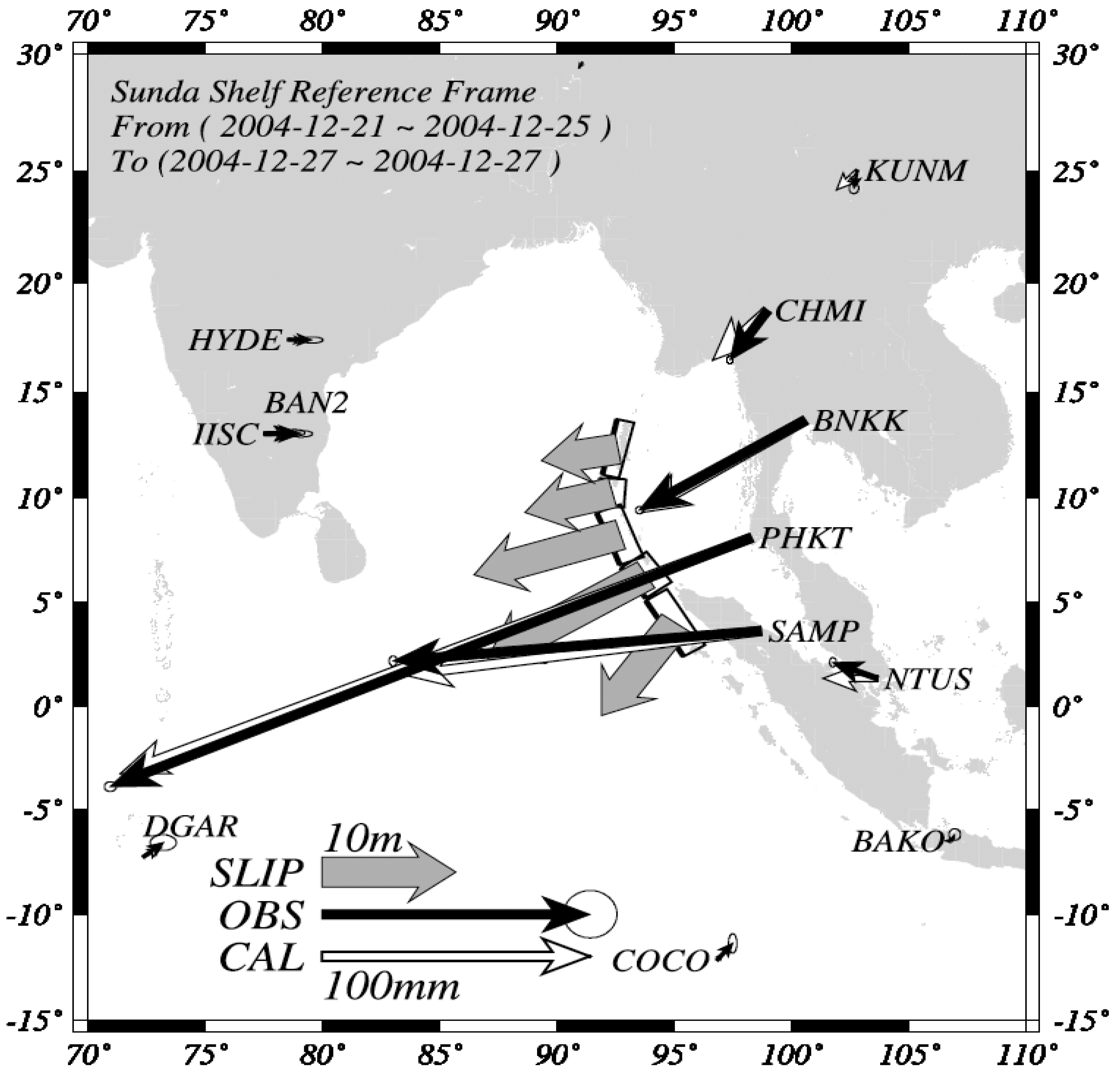
GPS data show that the Sumatra earthquake of 26 December 2004 (M = 9.0) was generated by a rupture of the Sunda subduction megathrust over a distance of >1,500 kilometers and a width of <150 kilometers. Megathrust slip exceeded 20 meters offshore northern Sumatra, mostly at depths shallower than 30 kilometers. Comparison of the geodetically and seismically inferred slip distribution indicates that approximately 30 % additional fault slip accrued in the 1.5 months following the 500-second-long seismic rupture [27].
Figure 11.
Co-seismic displacements from the Sumatra earthquake (M = 9.0, 26 December 2004, Indonesia). Solid and open arrows show observed by GPS and calculated displacements for the optimal model, respectively. Rectangles are surface projections of assumed fault segments whose upper margins are indicated by thick lines. Thick arrows are the estimated slip on each segment [28].
2.4. Gravity
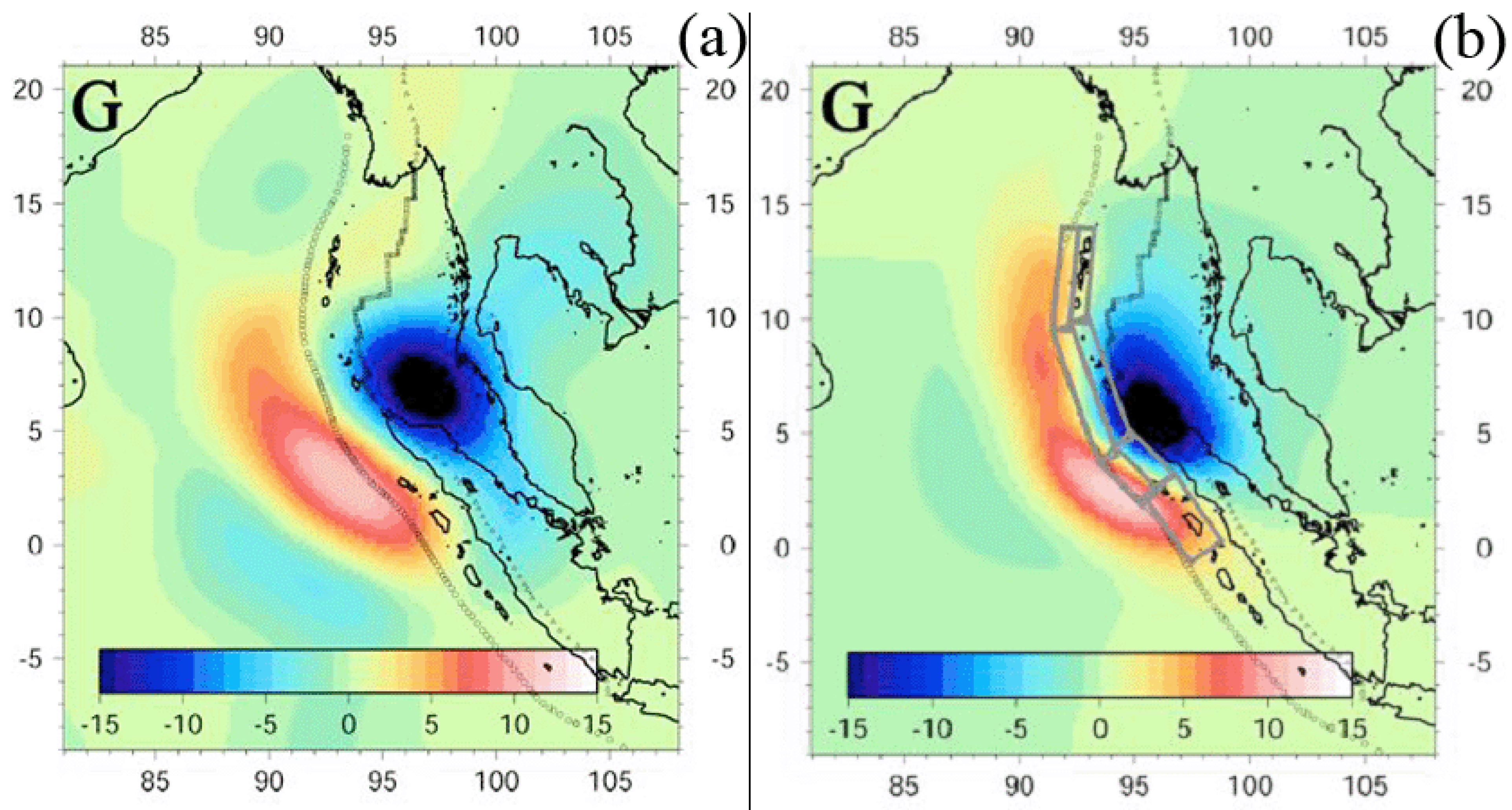
The detection of an earthquake by a space-based gravitation measurement was reported in 2006 [29]. The Gravity Recovery and Climate Experiment (GRACE) satellites observed a ± 15-microgalileo gravity change induced by the 2004 Sumatra earthquake (Figure 12). Co-seismic deformation produces sudden changes in the gravity field by vertical displacement of Earth's layered density structure and by changing the densities of the crust and mantle. GRACE's sensitivity to the long spatial wavelength of gravity changes resulted in roughly equal contributions of vertical displacement and dilatation effects in the gravity measurements. The GRACE observations provide evidence of crustal dilatation resulting from an undersea earthquake. GRACE is more sensitive (~50% signal retained) to the dilatation effect than to the vertical gravity change (a few %) from the Sumatra EQ co-seismic signals. The negative effect is due to density changes in the crust and the mantle, largely due to expansion of the crust.
Figure 12.
Satellite data showing the gravity changes for the Sumatra earthquake (M = 9.0, 26 December 2004, Indonesia). (a) A composite image from GRACE observed gravity change (±15 μgal). (b) Seismic model predicted gravity change at GRACE resolution [29].
Figure 12.
Satellite data showing the gravity changes for the Sumatra earthquake (M = 9.0, 26 December 2004, Indonesia). (a) A composite image from GRACE observed gravity change (±15 μgal). (b) Seismic model predicted gravity change at GRACE resolution [29].

3. Thermal Phenomena
The modern operational space-borne sensors in the TIR spectrum allow monitoring of the Earth’s thermal field with a spatial resolution of 0.5–5 km and with a temperature resolution of 0.12–0.5 °C. Surveys are repeated every 12 hours for the polar orbit satellites, and 30 minutes for geostationary satellites. The operational system of polar orbit satellites (two–four satellites in orbit) provides a whole globe survey at least every 6 hours or more frequently. Such sensors may closely monitor seismic prone regions and provide information about the changes in surface temperature associated with an impending earthquake.
Natural phenomena and data availability stimulated the analysis of the long time series of thermal images in relation to earthquake hazard. Historically, the first application of thermal images in earthquake study was carried out in the ‘80s for Middle Asia [30,31]. Later similar research was carried out in China [32,33], Japan [34], India [35,36], Italy [37], Spain and Turkey [38], USA [39] and other countries. Thermal observations from satellites indicate a significant change of the Earth's surface temperature and near-surface atmosphere layers. Significant thermal anomalies prior to earthquakes related to high seismic areas have been reported for all areas listed above.
3.1. Earth Surface
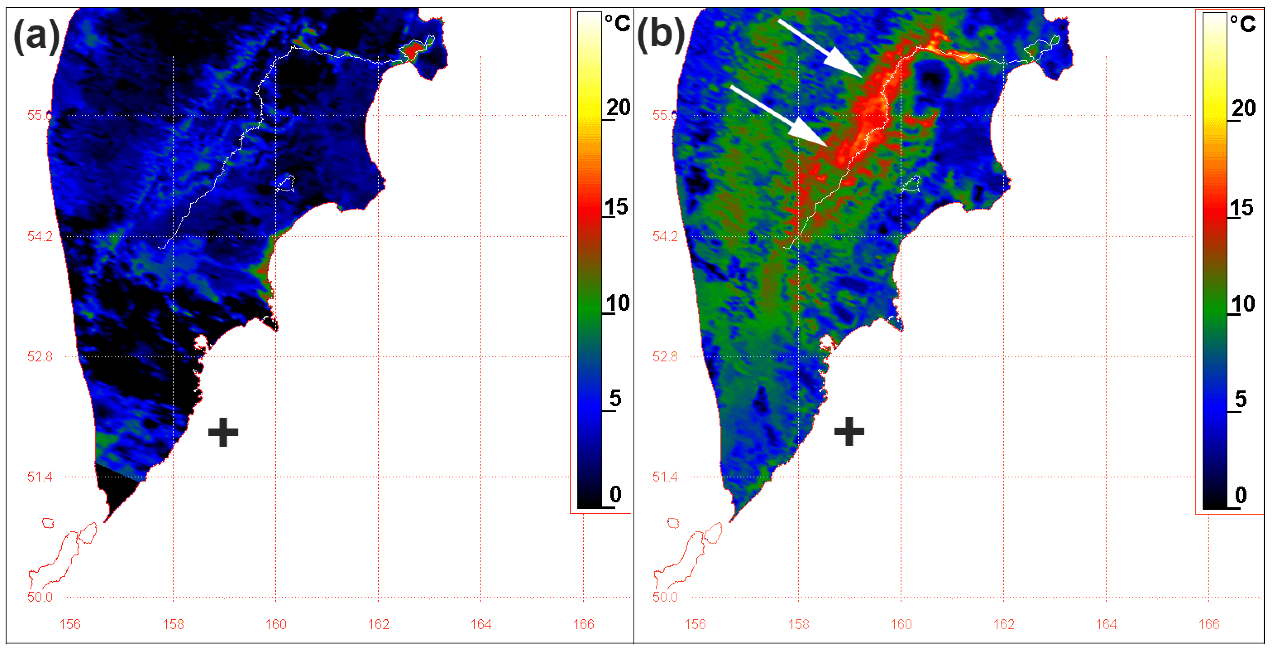
Satellite observations show the presence of TIR anomalies on the Kamchatka peninsula, Far East Russia, remarkable for its high seismicity, volcanic activity, geothermal fields, geysers, complex relief and bad weather conditions for satellite observations [40]. One example of clear thermal anomaly, related with the 21 Jun 1996 earthquake in Kamchatka is described below. A week before the shock the background distribution of land surface temperature (LST) was observed (Figure 13a). Immediately after the shock 22 Jun 1996 a large scale anomaly was detected in the basin of Kamchatka river (Figure 13b) at the centre of the peninsula. The valley of Kamchatka River is a famous artesian basin with numerous hot springs situated along the ‘thermal lines’. Ground observations confirmed satellite data: water temperature and debit of hot springs changed simultaneously with thermal anomaly variation [40].
Figure 13.
Thermal anomaly related with Kamchatka earthquake (M = 7.0, 21 Jun 1996, Far East, Russia). (a) Background situation, satellite NOAA-14, 14 Jun 1996, cross-earthquake epicenter 21 Jun 1996. (b) Thermal anomaly, satellite NOAA-14, 22 Jun 1996, arrows show thermal anomaly, cross-earthquake epicenter [40].

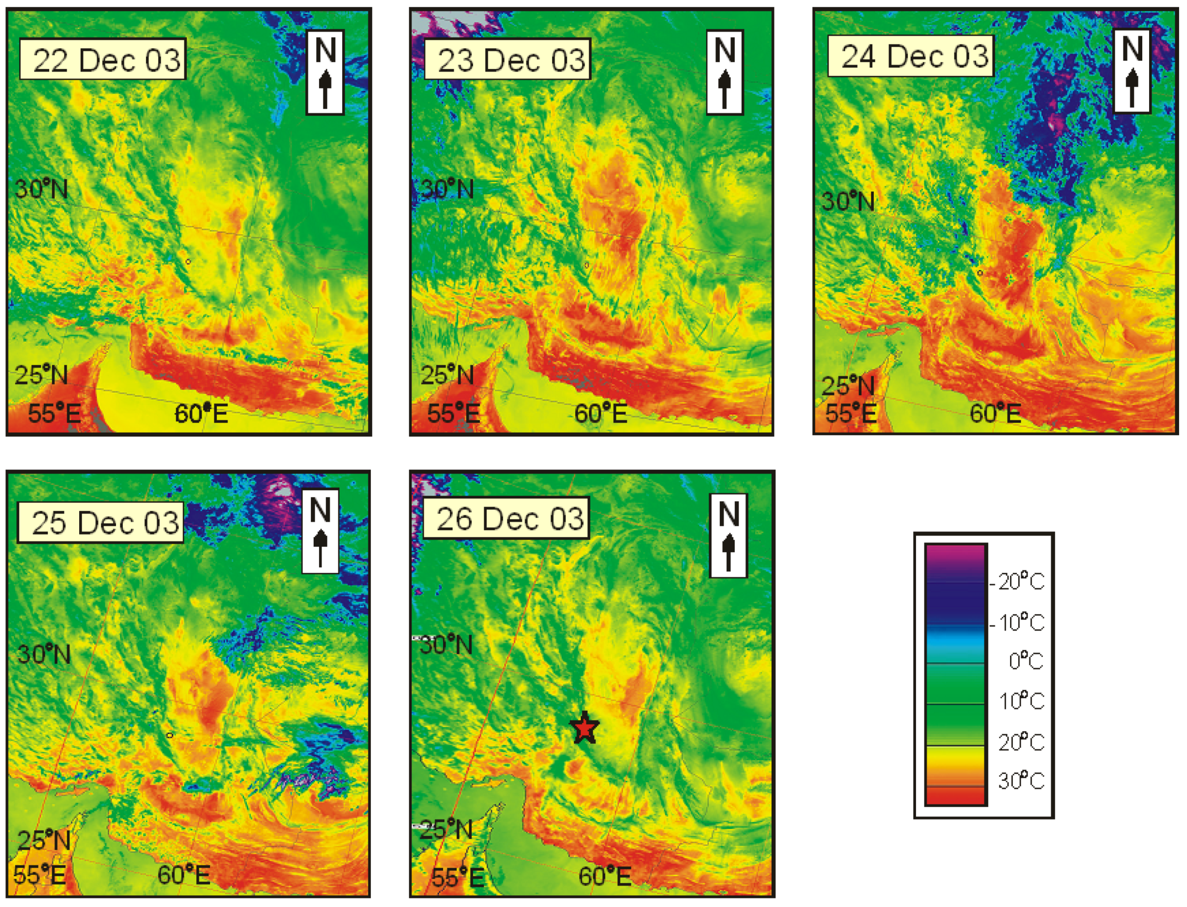
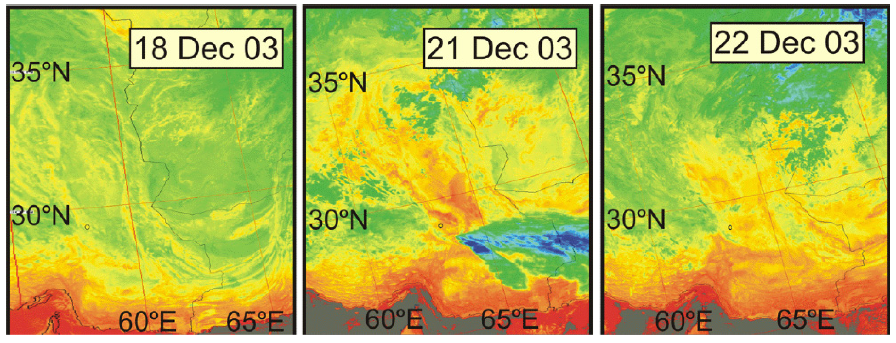
The destructive Bam earthquake in Iran took place on 26 December 2003. The magnitude of the earthquake was 6.6 and the city of Bam was destroyed. Analyses of the daytime and nighttime datasets for the Bam region showed a distinct anomaly in LST which appeared before the main shock [41]. The temperature increase was about 5–7 °C above the usual temperature of the region. At some places, the temperature was about 6–10 °C higher than the normal temperature of the region in that period of the year. In the nighttime maps, it was seen that on 18 December 2003 there was a complete normal temperature regime in the region (Figure 14). The appearance of an intense thermal anomaly was seen around the earthquake epicenter near Bam on 21 December 2003 (data was not available on 19 and 20 December 2003 for the same time of acquisition). Daytime LST time series maps show that the rise in temperature started on 22 December 2003 (Figure 15). The anomaly remained till 24 December 2003 (just two days before the earthquake). The normal temperature was around 22–25 °C on 21 December 2003. On 24 December 2003, the temperature was around 29–32 °C (about 7–10 °C higher than usual temperature of the region around that period of the year).
Figure 14.
Thermal anomalies associated with Bam earthquake (M = 6.6, 26 December 2003, Iran). NOAA-AVHRR daytime data, star indicate earthquake epicenter [41].
Figure 14.
Thermal anomalies associated with Bam earthquake (M = 6.6, 26 December 2003, Iran). NOAA-AVHRR daytime data, star indicate earthquake epicenter [41].

Figure 15.
Thermal anomalies associated with the Bam earthquake (M = 6.6, 26 December 2003, Iran). NOAA-AVHRR nighttime data, the star indicates the earthquake epicenter [41].
Figure 15.
Thermal anomalies associated with the Bam earthquake (M = 6.6, 26 December 2003, Iran). NOAA-AVHRR nighttime data, the star indicates the earthquake epicenter [41].


Tramutoli and colleagues have developed a robust satellite data analysis technique for space-time thermal anomalies on the Earth’s surface recorded by satellites months to weeks before the occurrence of earthquakes [37]. A robust satellite data analysis technique permits identification of space-time thermal infrared anomalies even under very variable observational and natural conditions. A robust estimator of TIR anomalies (RETIRA), ⊗(r,t), where r represents geographic coordinates of the image pixel center, t―is the time of acquisition of the satellite image, has been proposed first by Tramutoli [42]. In this way ⊗(r,t) gives the local excess of the current thermal signal compared with its historical mean value and weighted by its historical variability at the considered location.
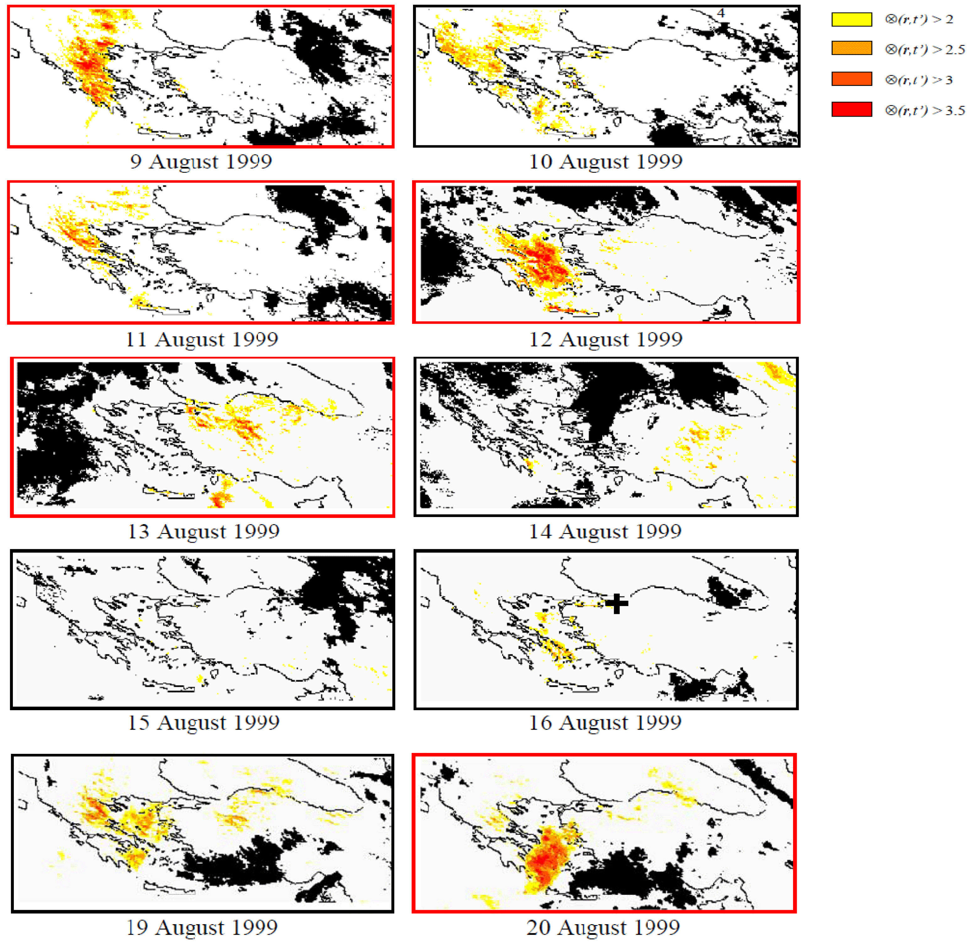
A statistically well-founded definition of thermal anomalies is given and proposed as a suitable tool for satellite thermal infrared surveys in seismically active regions. Eight years of Meteosat TIR observations have been analyzed in order to characterize the TIR signal behavior at each specific observation time and location. Space-time TIR signal transients have then been analyzed, both in the presence (validation) and in the absence of (confutation) seismic events, looking for possible space-time relationships. The devastating earthquake which occurred in Izmit, Turkey (M = 7.8, 17 August 1999) has been considered as a test case for validation (Figure 16). Quite intense (Signal/Noise > 3.5) and rare, spatially extensive and time persistent, TIR signal transients were identified, appearing eight days before the Izmit main shock in Greece (August 9th and 12th) and after the shock (August 19th and 20th).
Figure 16.
Results of the RETIRA index computation during August 1999 for the Izmit earthquake (M = 7.8, 17 August 1999, Turkey). Cloudy locations (no data) are depicted in black. Pixels with ⊗(r,t) > 3.5 are depicted in red. The black cross, on August 16th, indicates the epicentral area of the Izmit earthquake. Red boxes contour images showing pixels with ⊗(r,t) > 3.5. All scenes refer to Meteosat TIR observations collected at 24:00 GMT) [43].
Numerous thermal anomalies related with seismic activity were reported for other resent earthquakes: Colima, M = 7.8, 21 January 2003, Mexico [44]; Bhuj (Gujarat), M = 7.7, 26 January 2001, India [44,45]; Kashmir, M = 7.6, 8 October 2005, [46]; Sichuan, M = 8.0, 12 May 2008, China [47] and many others.
Cases studies of various thermal remote sensing methods applications for earthquakes were reported recently. Pinty et al. [48] have found a significant emergence of surface moisture growth after the Bhuj (Gujarat) earthquake, 26 January 2001, using MISR (Multi-angle Imaging SpectroRadiometer) data. Dey and Singh [49] found significant Surface Latent Heat Flux (SLHF) changes prior to the same earthquake. SLHF anomalies were also reported for the Colima earthquake, M = 7.8, 21 January 2003, Mexico [50] and the Tokachi-Oki earthquake, M = 8.3, 25 September 2003, Japan [51]. Reanalysis of climatic data are also involved in thermal data processing in seismic processes [52].
Satellite thermal survey has a relatively long history of applications in seismology. Most of its advantages and deficiencies are well known. Two main problems limit thermal data utilization: cloud penetration and geological situation. The first issue will be overcome with microwave radiometers in the future. Spatial resolution of microwave devices is too coarse now. The second problem is a fundamental one. There are no strong correlations between seismic activity and thermal anomalies on the Earth’s surface. More accurately, we have correlations for some area, for not for others. Surface conditions such as vegetation, precipitations, wind, etc. also strongly influence thermal effects.
3.2. Sea Surface
The sea surface is considered as a more complex object for satellite data applications for seismology. The sea surface temperature depends strongly on weather conditions and sea currents. Due to high thermal inertia all processes of water heating and cooling take place much slower than on the ground.
Figure 17.
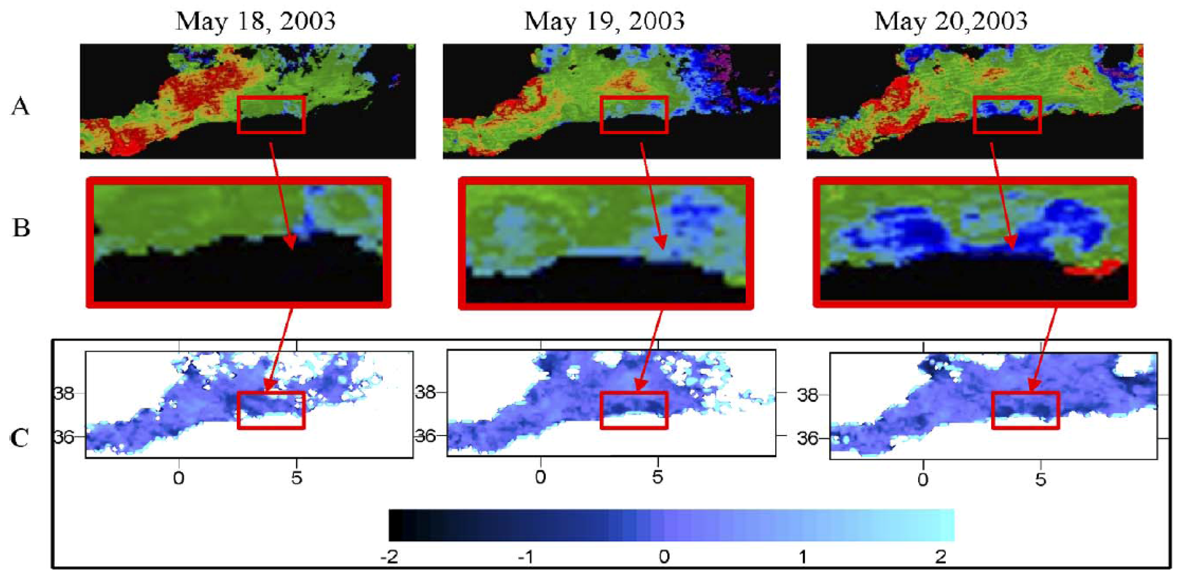
Sea surface temperature variation for Boumerdes earthquake (M = 6.8, 21 May 2003, Algeria). MODIS Terra LST for May 18, 19 and 20 in near zone to the epicenter. (a) Map of 4.5 km nighttime girded SST data, with red rectangle marking the upwelling area. Land is masked with black color. (b) Zoom in the epicentral area with cooling the surface temperature (blue color). (c) SST residual computed for the same days by the method of median polish [44].
Figure 17.
Sea surface temperature variation for Boumerdes earthquake (M = 6.8, 21 May 2003, Algeria). MODIS Terra LST for May 18, 19 and 20 in near zone to the epicenter. (a) Map of 4.5 km nighttime girded SST data, with red rectangle marking the upwelling area. Land is masked with black color. (b) Zoom in the epicentral area with cooling the surface temperature (blue color). (c) SST residual computed for the same days by the method of median polish [44].

Sea surface temperatures (SST) were analyzed for the Boumerdes earthquake (northern Algeria, 21 May 2003, M = 6.8 [44]). Statistical analysis was preformed to estimate the SST variability during the period of 90 days around 21 May 2003. Night images of Terra/MODIS for May 18, 19 and 20 were shown as the land was masked with black (Figure 17). The decrease of SST with amplitude –2 °C was observed on locations close to the epicenter and this temperature decrease pattern could not be seen before or after the main shock. The statistical analysis confirms that a few days before the main shock there were local up-wellings of cold water with an average SST –2 °C in comparison with the background mean temperature. Some other examples of SST anomalies, mostly negative, related with earthquake were reported by Ouzounov and Freund [53].
Figure 18.
Surface latent heat flux anomalies for the Sumatra earthquake (M = 9.0, 26 December 2004, Indonesia). (a) SLHF anomaly on 7 December 2004. (b) Time series of wavelet analysis of SLHF for the period from 27 December 2003 to 25 December 2004 [55].
Figure 18.
Surface latent heat flux anomalies for the Sumatra earthquake (M = 9.0, 26 December 2004, Indonesia). (a) SLHF anomaly on 7 December 2004. (b) Time series of wavelet analysis of SLHF for the period from 27 December 2003 to 25 December 2004 [55].
Singh et al. [54] found changes in water color and Earth's surface related to Bhuj (Gujarat) earthquake of January 26 using IRS satellite data. Numerous sea surface parameters variations were discussed in relation with Sumatra earthquake, 2004, from SLHF (Figure 18) till chlorophyll-a concentrations [55].
3.3. Atmosphere
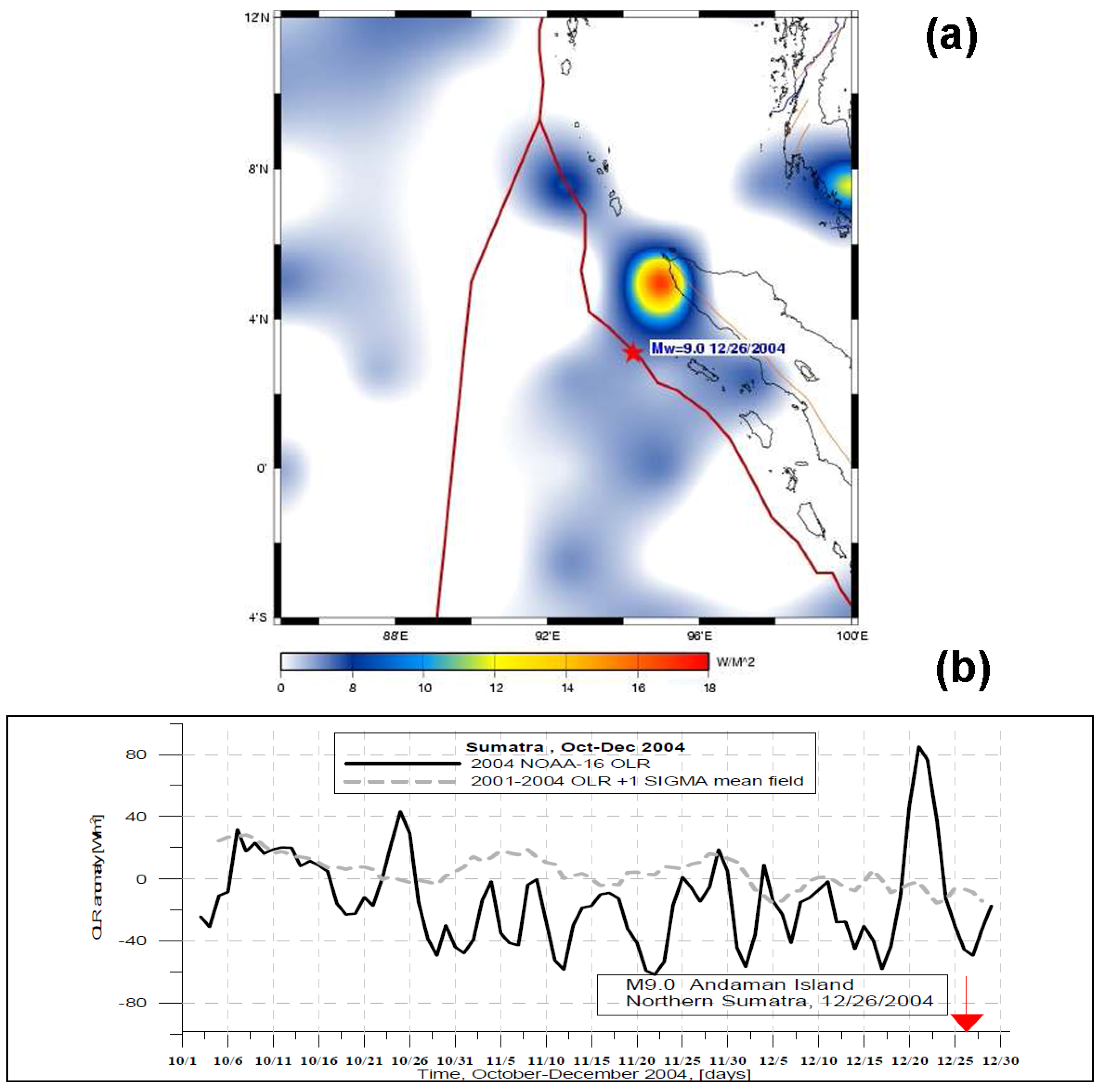
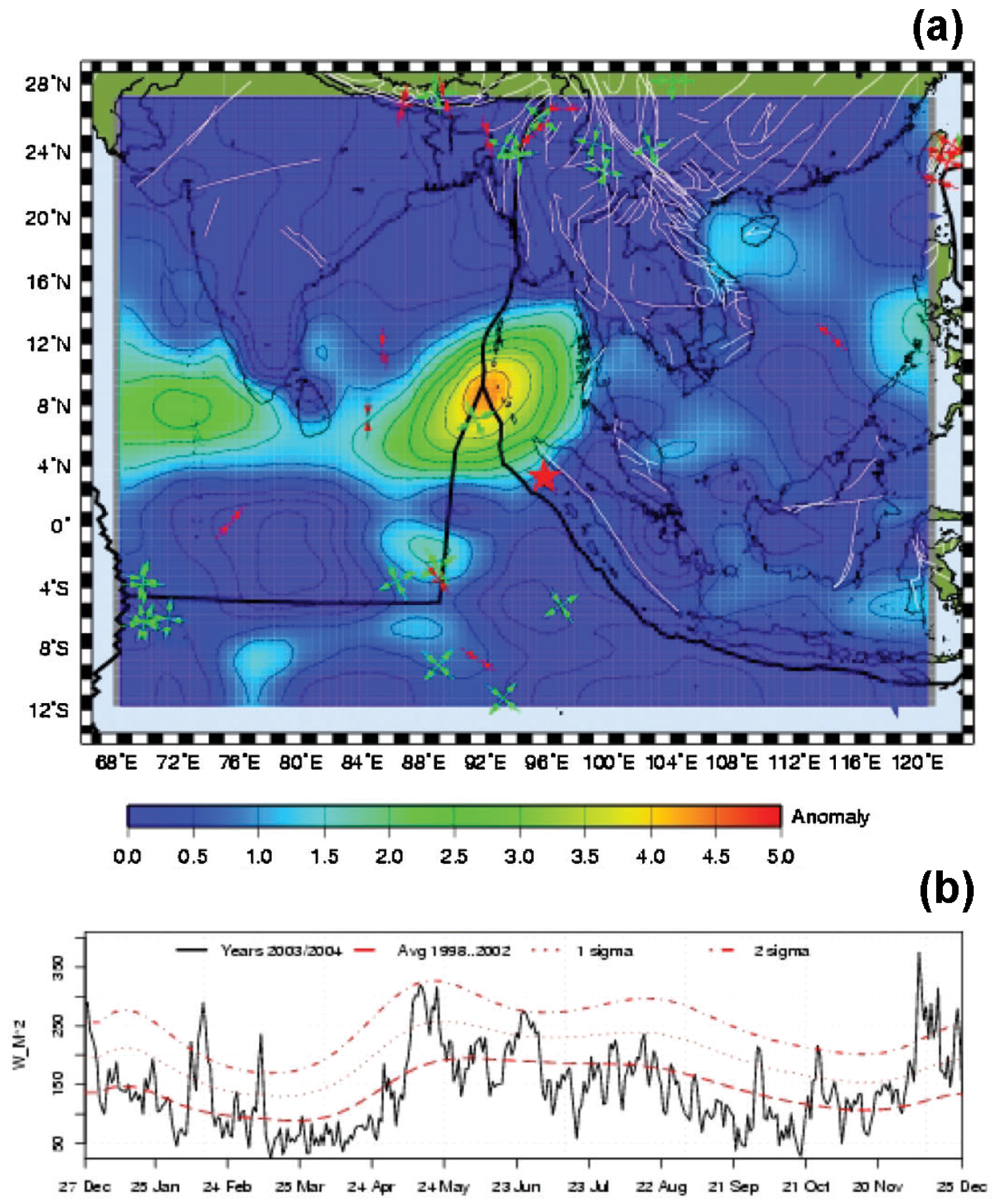
Thermal anomalies before strong earthquakes are observed at different levels, starting from the ground surface up to the top of clouds altitude. All kinds of anomalies were registered repeatedly by many researchers before different earthquakes by remote sensing satellite techniques on the earth and sea surface. The most promising in the present moment is the Outgoing Longwave Radiation (OLR) anomaly measured at the top of clouds level [56]. Its advantage is that it is measured within the infrared transparency window of 8–12 microns and does not separate clouds. OLR is currently mapped by the AIRS (Atmospheric Infrared Sounder) launched into orbit in 2002. AIRS is one of six instruments on board the Aqua satellite, part of the NASA Earth Observing System. One of the best examples of OLR anomalies is related with the Sumatra earthquake in 2004 (Figure 19).
Figure 19.
Outgoing longwave radiation anomaly for the Sumatra earthquake (M = 9.0, 26 December 2004, Indonesia). (a) Map of OLR monthly variations for November 2004, month prior to the shock. (b) Time-series of daily OLR anomaly for 1 October 2004–31 December 2004 over the epicenter [56].
Figure 19.
Outgoing longwave radiation anomaly for the Sumatra earthquake (M = 9.0, 26 December 2004, Indonesia). (a) Map of OLR monthly variations for November 2004, month prior to the shock. (b) Time-series of daily OLR anomaly for 1 October 2004–31 December 2004 over the epicenter [56].

It is difficult to expect that something like a ground surface temperature increase by 3–5 degrees or infrared emission emitted by rocks due to deformation can provide at an altitude of 12 km the energy flux within the range 4–80 W/m2 which was measured experimentally. Such an amount of energy could only be provided by some process taking place directly in the atmosphere.
Dey et al. [57] found changes in the total water vapour column after the Bhuj (Gujarat) earthquake. Water content was retrieved by SSM/I microwave radiometer on the Tropical Rainfall Measuring Mission (TRMM) satellite. Okada et al. [58] found changes in atmospheric aerosol parameters after the Bhuj (Gujarat) earthquake. Aerosols above the sea surface were revealed on the base SeaWiFS satellite data. A few examples of ozone concentrations changes measured by TOMS related with earthquakes have been reported by Tronin [59].
4. Electromagnetics
Electromagnetic observations do not belong to remote sensing. Nevertheless the role of these methods in earthquake research is very important. One can find a comprehensive review on seismo-electromagnetics presented by Uyeda, Nagao and Kamogawa [63]. The DEMETER mission [64] successfully executes a science program on seismo-ionoshperic research [65,66].
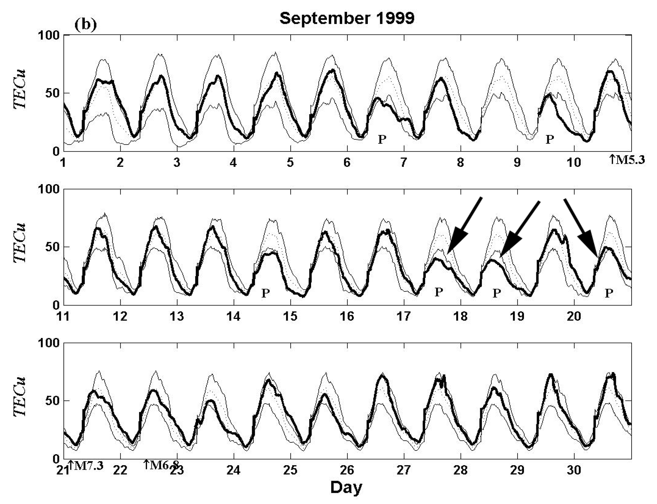
Total electron content (TEC) is one the main parameters studied in relation with earthquakes [6]. GPS observations at the moment are the main tool for TEC measurements. The density of GPS stations increases every year, which allows for restoring the 3D ionosphere structure. An excellent example of TEC variation (Figure 20) was represented for the Chi-Chi earthquake [67]. Modern TEC applications can be found in the publications of Liu [68,69,70]. On the other hand the constellation of satellites with scatterometers like QuikSCAT generates TEC images above sea surface as side effects.
Figure 20.
The variations of TEC observed in September 1999 for the Chi-Chi earthquake (M = 7.6, 20 September 1999, Taiwan). 1 TECu = 1016 el/m2. Arrows show TEC anomalies [67].
Figure 20.
The variations of TEC observed in September 1999 for the Chi-Chi earthquake (M = 7.6, 20 September 1999, Taiwan). 1 TECu = 1016 el/m2. Arrows show TEC anomalies [67].

5. Discussion
A wide spectrum of satellite remote sensing methods are applied in seismology nowadays. The value of these methods for earthquake research is varied. Optical methods have limited applications, mostly for rapid assessment of damages in an epicentral zone. Other applications such as alignment analysis and cloud form analysis related with earthquakes do not have an adequate scientific basis for seismological application. Vigorous extension of InSAR methods applications in seismology is observed now. Modern radar systems in conjunction with GPS/GLONASS will provide whole seismic cycle monitoring. Broad application of InSAR methods is limited by the high data cost and complex data analysis. Thermal satellite data applications are developing in two directions at the moment: thermal anomalies in seismic fault research and emitted longwave radiation measurements in seismic zones. Thermal anomalies research in seismic faults is developing in the direction of seismic activity monitoring and close integration with ground observations. Emitted longwave radiation observations demonstrate promising results, but data accumulation is required. The nature of ongoing longwave radiation anomalies remains unclear.
Some common remarks on satellite data application in seismology can be made: (1) The level of automatic data processing is insufficient. There is still too much manual labour and author arbitrariness in data processing—this concerns both exotic earthquake cloud analysis and high technique radar methods. Some results are irreproducible. (2) There is a weak physical and geological basis for many of the proposed methods. The nature and driving forces of some phenomena need clarification and connection with current understanding of physics and geology.
6. Conclusions
This review of modern remote sensing techniques in seismology demonstrates the following: (1) remote sensing methods are being broadly used for earthquake research; (2) a wide spectra of remote sensing methods are applied—from optical sensors to radar systems; (3) the list of parameters studied by remote sensing are: surface deformation (both vertical and horizontal), surface temperature, various heat fluxes on the Earth’s and top clouds surfaces and some others; (4) future development of remote sensing application for earthquakes related with new directions: L-band radar systems, high-resolution microwave radiometers, gas analyzers; (5) we will probably again approach an epoch of “belief” in earthquake prediction, where remote sensing can play a key role due to its global scope, calibration, and automatic data processing.
The described processes in the ionosphere, atmosphere, hydrosphere and lithosphere associated with earthquakes represent the fundamental science issue of lithosphere-atmosphere-ionosphere coupling. The solution of this problem is quite far away. We can mention specifically the problems of the nature of thermal anomalies, the nature of emitted longwave radiation anomalies, ionosphere-lithosphere coupling and so on. All these issues interface with the problem of understanding the nature of earthquakes.
References
- Showalter, P.S. Remote sensing’s use in disaster research: a review. Disaster Prevent. Manage. 2001, 10, 21–29. [Google Scholar] [CrossRef]
- Paylor, E.D., II; Evans, D.L.; Tralli, D.M. Remote sensing and geospatial information for natural hazards characterization. ISPRS J. Photogramm. Remote Sens. 2005, 59, 181–253. [Google Scholar] [CrossRef]
- IGOS. International Global Observation Strategy Geohazards Theme Report; ESA/UNESCO: European Space Agency, Paris, France, 2004; p. 54. [Google Scholar]
- Joyce, K.E.; Belliss, S.E.; Samsonov, S.V.; McNeill, S.J.; Glassey, P.J. A review of the status of satellite remote sensing and image processing techniques for mapping natural hazards and disasters. Prog. Phys. Geog. 2009, 33, 183–207. [Google Scholar] [CrossRef]
- Tronin, A.A. Remote sensing and earthquakes: a review. Phys. Chem. Earth 2006, 31, 138–142. [Google Scholar] [CrossRef]
- Hayakawa, M. Atmospheric and Ionospheric Electromagnetic Phenomena Associated with Earthquakes; Terra Sci. Pub. Co. Ltd.: Tokyo, Japan, 1999; p. 996. [Google Scholar]
- Seismo Electromagnetics: Lithosphere-Atmosphere-Ionosphere Coupling; Hayakawa, M.; Molchanov, O.A. (Eds.) Terra Science Publishing Co. Ltd.: Tokyo, Japan, 2002; p. 477.
- Clark, M.M. Finding active faults using aerial photographs. Earthqua. Inf. Bull. 1978, 10, 169–173. [Google Scholar]
- Trifonov, V.G. Active faults in Eurasia: general remarks. Tectonophysics 2004, 380, 123–130. [Google Scholar] [CrossRef]
- Trifonov, V.G.; Makarov, V.I.; Kojurin, A.I.; Skobelev, S.F.; Schulz, S.S., Jr. Aerospace Research of Seismic Zones; Nauka: Moscow, USSR, 1988; p. 133. (in Russian) [Google Scholar]
- Saraf, A.K. IRS-1C-PAN Depicts Chamoli earthquake induced landslides in Garhwal Himalayas, India. Int. J. Remote Sens. 2000, 21, 2345–2352. [Google Scholar] [CrossRef]
- Van Puymbroeck, N.; Michel, R.; Binet, R.; Avouac, J.P.; Taboury, J. Measuring earthquakes from optical satellite images. Appl. Opt. Inf. Process. 2000, 39, 1–14. [Google Scholar] [CrossRef]
- Michel, R.; Avouac, J.P. Deformation due to the 17 August Izmit, Turkey, earthquake measured from SPOT images. J. Geophys. Res. 2002. [Google Scholar] [CrossRef]
- Dominguez, S.; Avouac, J.P.; Michel, R. Horizontal coseismic deformation of the 1999 Chi-Chi earthquake measured from SPOT satellite images: Implications for the seismic cycle along the western foothills of Central Taiwan. J. Geophys. Res. 2003. [Google Scholar] [CrossRef]
- Arellano-Baeza, A.A.; Zverev, A.T.; Malinnikov, V.A. Study of changes in the lineament structure, caused by earthquakes in South America by applying the lineament analysis to the Aster (Terra) satellite data. Adv. Space Res. 2006, 37, 690–697. [Google Scholar] [CrossRef]
- Massonnet, D.; Rossi, M.; Carmona, C.; Adragna, F.; Peltzer, G.; Feigl, K.; Rabaute, T. The displacement field of the Landers earthquake mapped by radar interferometry. Nature 1993, 364, 138–142. [Google Scholar] [CrossRef]
- Peltzer, G.; Hudnut, K.; Feigl, K. Analysis of coseismic surface displacement gradients using radar interferometry: New insights into the Landers earthquake. J. Geophys. Res. 1994, 99, 21971–21981. [Google Scholar] [CrossRef]
- Tobita, M.; Fujiwara, S.; Ozawa, S.; Rosen, P.A.; Fielding, E.J.; Werner, C.L.; Murakami, M.; Nakagawa, H.; Nitta, K.; Murakami, M. Deformation of the 1995 North Sakhalin earthquake detected by JERS-1/SAR interferometry. Earth Planets Space 1998, 50, 313–325. [Google Scholar] [CrossRef]
- Schmidt, D.A.; Bürgmann, R. InSAR constraints on the source parameters of the 2001 Bhuj earthquake. Geophys. Res. Lett. 2006, 33, L02315. [Google Scholar] [CrossRef]
- Stramondo, S.; Moro, M.; Tolomei, C.; Cinti, F.R.; Doumaz, F. InSAR surface displacement field and fault modelling for the 2003 Bam earthquake (southeastern Iran). J. Geodynamics 2005, 40, 347–353. [Google Scholar] [CrossRef]
- Chini, M.; Bignami, C.; Stramondo, S.; Pierdicca, N. Uplift and subsidence due to the 26 December 2004 Indonesian earthquake detected by SAR data. Int. J. Remote Sens. 2008, 29, 3891–3910. [Google Scholar] [CrossRef]
- Kuzuoka, S.; Mizuno, T. Land Deformation Monitoring Using PSInSAR Technique. In Proceedings of International Symposium on Monitoring, Prediction and Mitigation of Disasters by Satellite Remote Sensing, Awaji, Hyogo, Japan, January 2004; pp. 176–181.
- Tsai, Y.B.; Liu, J.Y.; Ma, K.F.; Yen, H.Y.; Chen, K.S.; Chen, Y.I.; Lee, C.P. Precursory phenomena associated with the 1999 Chi-Chi earthquake in Taiwan as identified under iSTEP Program. Phys. Chem. Earth 2006, 31, 365–377. [Google Scholar] [CrossRef]
- de Michele, M.; Raucoulesa, D.; Salichon, J.; Lemoine, A.; Aochia, H. Using INSAR for seismotectonic observations over the Mw 6.3 Parkfield earthquake (28/09/2004), California. In Proceedings of Commission IV ISPRS Congress, Beijing, China, July 2008; Available online: http://www.isprs.org/congresses/beijing2008/proceedings/4_pdf/265.pdf (accessed on 15 November 2009).
- Fielding, E.J.; Lundgren, P.R.; Bürgmann, R.; Funning, G.J. Shallow fault-zone dilatancy recovery after the 2003 Bam, Iran earthquake. Nature 2009, 458, 64–68. [Google Scholar] [CrossRef] [PubMed]
- Ozawa, S.; Murakami, M.; Kaidzu, M.; Hatanaka, Y. Transient crustal deformation in Tokai region, centeral Japan, until May 2004. Earth Planets Space 2005, 57, 909–915. [Google Scholar] [CrossRef]
- Subarya, C.; Chlieh, M.; Prawirodirdjo, L.; Avouac, J.-P.; Bock, Y.; Sieh, K.; Meltzner, A.J.; Natawidjaja, D.H.; McCaffrey, R. Plate-boundary deformation associated with the great Sumatra-Andaman earthquake. Nature 2006, 440, 46–51. [Google Scholar] [CrossRef] [PubMed]
- Hashimoto, M.; Choosakul, N.; Hashizume, M.; Takemoto, S.; Takiguchi, H.; Fukuda, Y.; Fujimori, K. Crustal deformations associated with the great Sumatra-Andaman earthquake deduced from continuous GPS observation. Earth Planets Space 2006, 58, 127–139. [Google Scholar] [CrossRef]
- Han, S.-C.; Shum, C.K.; Bevis, M.; Ji, C.; Kuo, C.-Y. Crustal Dilatation Observed by GRACE after the 2004 Sumatra-Andaman Earthquake. Science 2006, 313, 658–662. [Google Scholar] [CrossRef] [PubMed]
- Gorny, V.I.; Salman, A.G.; Tronin, A.A.; Shilin, B.V. The earth’s outgoing IR radiation as an indicator of seismic activity. Proc. Acad. Sci. USSR 1988, 301, 67–69. [Google Scholar]
- Tronin, A.A. Satellite thermal survey—a new tool for the studies of seismoactive regions. Int. J. Remote Sens. 1996, 17, 1439–1455. [Google Scholar] [CrossRef]
- Quang, Z.; Xu, X.; Dian, C. Thermal infrared anomaly precursors of impending earthquakes. Chin. Sci. Bull. 1991, 36, 319–323. [Google Scholar] [CrossRef]
- Qiang, Z.; Du, L.-T. Earth degassing, forest fire and seismic activities. Earth Science Frontiers 2001, 8, 235–245. [Google Scholar]
- Tronin, A.A.; Hayakawa, M.; Molchanov, O.A. Thermal IR satellite data application for earthquake research in Japan and China. J. Geodynamics 2002, 33, 519–534. [Google Scholar] [CrossRef]
- Saraf, A.K.; Choudhury, S. Earthquakes and thermal anomalies. Geospatial Today 2003, 2, 18–20. [Google Scholar]
- Singh, R.P.; Ouzounov, D. Earth processes in wake of Gujarat earthquake reviewed from space. EOS Trans. Amer. Geophys. Union 2003, 84, 244. [Google Scholar] [CrossRef]
- Tramutoli, V.; Bello, G.D.; Pergola, N.; Piscitelli, S. Robust satellite techniques for remote sensing of seismically active areas. Ann. Geofis. 2001, 44, 295–312. [Google Scholar]
- CORDIS RTD-PROJECTS. Regular Update of Seismic Hazard Maps through Thermal Space Observations; European Communities: Madrid, Spain, Project Reference: ENV4980741; 2000. [Google Scholar]
- Ouzounov, D.; Freund, F. Mid-infrared emission prior to strong earthquakes analyzed by remote sensing data. Adv. Space Res. 2003, 33, 268–273. [Google Scholar] [CrossRef]
- Tronin, A.A.; Biagi, P.F.; Molchanov, O.A.; Khatkevich, Y.M.; Gordeeev, E.I. Temperature variations related to earthquakes from simultaneous observation at the ground stations and by satellites in Kamchatka area. Phys. Chem. Earth 2004, 29, 501–506. [Google Scholar] [CrossRef]
- Saraf, A.K.; Rawat, V.; Banerjee, P.; Choudhury, S.; Panda, S.K.; Dasgupta, S.; Das, J.D. Satellite detection of earthquake thermal precursors in Iran. Nat. Hazard 2008, 47, 119–135. [Google Scholar] [CrossRef]
- Tramutoli, V. Robust AVHRR Techniques (RAT) for environmental monitoring: theory and applications. In Earth Surface Remote Sensing II; Cecchi, G., Zilioli, E, Eds.; SPIE: Barcelona, Spain, 1998; pp. 101–113. [Google Scholar]
- Tramutoli, V.; Cuomo, V.; Filizzola, C.; Pergola, N.; Pietrapertosa, C. Assessing the potential of thermal infrared satellite surveys for monitoring seismically active areas. The case of Kocaeli (İzmit) earthquake, August 17, 1999. Remote Sens. Environ. 2005, 96, 409–426. [Google Scholar] [CrossRef]
- Ouzounov, D.; Bryant, N.; Logan, T.; Pulinets, S.; Taylor, P. Satellite thermal IR phenomena associated with some of the major earthquakes in 1999–2003. Phys. Chem. Earth 2006, 31, 154–163. [Google Scholar] [CrossRef]
- Saraf, A.K.; Choudhury, S. NOAA-AVHRR detects thermal anomaly associated with 26 January, 2001 Bhuj Earthquake, Gujarat, India. Int. J. Remote Sens. 2005, 26, 1065–1073. [Google Scholar] [CrossRef]
- Panda, S.K.; Choudhury, S.; Saraf, A.K.; Das, J.D. MODIS land surface temperature data detects thermal anomaly preceding 08 October 2005 Kashmir earthquake. Int. J. Remote Sens. 2007, 28, 4587–4596. [Google Scholar] [CrossRef]
- Wei, L.; Guo, J.; Liu, J.; Lu, Z.; Li, H.; Cai, H. Satellite thermal infrared earthquake precursor to the Wenchuan Ms 8.0 earthquake in Sichuan, China, and its analysis on geodynamics. Acta Geol. Sinica-Engl. Ed. 2009, 83, 767–775. [Google Scholar] [CrossRef]
- Pinty, B.; Gobron, N.; Verstraete, M.M.; Mélin, F.; Widlowski, J.-L.; Govaerts, Y.; Diner, D.J.; Fielding, E.; Nelson, D.L.; Madariaga, R.; Tuttle, M.P. Observing earthquake-related dewatering using MISR/Terra satellite Data. EOS Trans. Amer. Geophys. Union 2003, 84, 37–48. [Google Scholar] [CrossRef]
- Dey, S.; Singh, R.P. Surface latent heat flux as an earthquake precursor. Nat. Hazards Earth Syst. 2003, 3, 749–755. [Google Scholar] [CrossRef]
- Pulinets, S.A.; Ouzounov, D.; Ciraolo, L.; Singh, R.; Cervone, G.; Leyva, A.; Dunajecka, M.; Karelin, A.V.; Boyarchuk, K.A.; Kotsarenko, A. Thermal, atmospheric and ionospheric anomalies around the time of the Colima M7.8 earthquake of 21 January 2003. Ann. Geophys. 2006, 24, 835–849. [Google Scholar] [CrossRef]
- Cervone, G.; Maekawa, S.; Singh, R.; Hayakawa, M.; Kafatos, M.; Shavets, A. Surface latent heat flux and nighttime LF anomalies prior to the Mw = 8.3 Tokachi-Oki earthquake. Nat. Hazards Earth Syst. Sci. 2006, 6, 109–114. [Google Scholar] [CrossRef]
- Ma, W.; Ma, W.; Zhao, H.; Li, H. Temperature changing process of the Hokkaido (Japan) earthquake on 25 September 2003. Nat. Hazards Earth Syst. Sci. 2008, 8, 985–989. [Google Scholar] [CrossRef]
- Ouzounov, D.; Freund, F. Mid-infrared emission prior to strong earthquakes analyzed by remote sensing data. Adv. Space Res. 2004, 33, 268–273. [Google Scholar] [CrossRef]
- Singh, R.P.; Bhoi, S.; Sahoo, A.K. Changes observed on land and ocean after Gujarat earthquake of January 26, 2001 using IRS data. Int. J. Remote Sens. 2002, 23, 3123–3128. [Google Scholar] [CrossRef]
- Singh, R.P.; Cervone, G.; Kafatos, M.; Prasad, A.K.; Sahoo, A.K.; Sun, D.; Tang, D.L.; Yang, R. Multi-sensor studies of the Sumatra earthquake and tsunami of 26 December 2004. Int. J. Remote Sens. 2007, 28, 2885–2896. [Google Scholar] [CrossRef]
- Ouzounov, D.; Liu, D.; Kang, C.; Cervone, G.; Kafatos, M.; Taylor, P. Outgoing long wave radiation variability from IR satellite data prior to major earthquakes. Tectonophysics 2007, 431, 211–220. [Google Scholar] [CrossRef]
- Dey, S.; Sarkar, S.; Singh, R.P. Anomalous changes in column water vapor after Gujarat earthquake. Adv. Space Res. 2004, 33, 274–278. [Google Scholar] [CrossRef]
- Okada, Y.; Mukai, S.; Singh, R.P. Changes in atmospheric aerosol parameters after Gujarat earthquake of January 26, 2001. Adv. Space Res. 2004, 33, 254–258. [Google Scholar] [CrossRef]
- Tronin, A.A. Atmosphere-litosphere coupling. Thermal anomalies on the earth surface in seismic processes. In Seismo Electromagnetics: Lithosphere-Atmosphere-Ionosphere Coupling; Hayakawa, M., Molchanov, O.A., Eds.; TERRAPUB: Tokyo, Japan, 2002; pp. 173–176. [Google Scholar]
- Morozova, L.I. Features of atmo-lithmospheric relationships during periods of strong Asian earthquakes. Izvestiya, Phys. Solid Earth 1996, 5, 63–68. [Google Scholar]
- Guo, G.; Wang, B. Cloud anomaly before Iran earthquake. Int. J. Remote Sens. 2008, 29, 1921–1928. [Google Scholar] [CrossRef]
- Gup, G.; Xie, G. Earthquake cloud over Japan detected by satellite. Int. J. Remote Sens. 2007, 28, 5375–5376. [Google Scholar] [CrossRef]
- Uyeda, S.; Nagao, T.; Kamogawa, M. Short-term earthquake prediction: current status of seismo-electromagnetics. Tectonophysics 2009, 470, 205–213. [Google Scholar] [CrossRef]
- Parrot, M. The micro-satelitte DEMETER. J. Geodynamics 2002, 33, 535–541. [Google Scholar] [CrossRef]
- Molchanov, O.; Rozhnoi, A.; Solovieva, M.; Akentieva, O.; Berthelier, J.J.; Parrot, M.; Lefeuvre, F.; Biagi, P.F.; Castellana, L.; Hayakawa, M. Global diagnostics of the ionospheric perturbations related to the seismic activity using the VLF radio signals collected on the DEMETER satellite. Nat. Hazards Earth Syst. Sci. 2006, 6, 745–753. [Google Scholar] [CrossRef]
- Parrot, M.; Berthelier, J.J.; Lebreton, J.P.; Sauvaud, J.A.; Santolík, O.; Blecki, J. Examples of unusual ionospheric observations made by the DEMETER satellite over seismic regions. Phys. Chem. Earth 2006, 31, 486–495. [Google Scholar] [CrossRef]
- Liu, J.; Chuo, Y.; Shan, S.; Tsai, Y.; Chen, Y.; Pulinets, S.; Yu, S. Pre-earthquake ionospheric anomalies registered by continuous GPS TEC measurements. Ann. Geophys. 2004, 22, 1585–1593. [Google Scholar] [CrossRef]
- Liu, J.Y.; Tsai, Y.B.; Chen, S.W.; Lee, C.P.; Chen, Y.C.; Yen, H.Y.; Chang, W.Y.; Liu, C. Giant ionospheric disturbances excited by the M9.3 Sumatra earthquake of 26 December 2004. Geophys. Res. Lett. 2006, 33, L02103. [Google Scholar] [CrossRef]
- Liu, J.-Y.; Tsai, Y.-B.; Ma, K.-F.; Chen, Y.-I.; Tsai, H.-F.; Lin, C.-H.; Kamogawa, M.; Lee, C.-P. Ionospheric GPS total electron content (TEC) disturbances triggered by the 26 December 2004 Indian Ocean tsunami. J. Geophys. Res. 2006, 111, A05303. [Google Scholar] [CrossRef]
- Liu, J.Y.; Chen, Y.I.; Chen, C.H.; Liu, C.Y.; Chen, C.Y.; Nishihashi, M.; Li, J.Z.; Xia, Y.Q.; Oyama, K.I.; Hattori, K.; Lin, C.H. Seismoionospheric GPS total electron content anomalies observed before the 12 May 2008 Mw7.9 Wenchuan earthquake. J. Geophys. Res. 2009, 114, A04320. [Google Scholar]
© 2010 by the authors; licensee Molecular Diversity Preservation International, Basel, Switzerland. This article is an open-access article distributed under the terms and conditions of the Creative Commons Attribution license (http://creativecommons.org/licenses/by/3.0/).
Share and Cite
MDPI and ACS Style
Tronin, A.A. Satellite Remote Sensing in Seismology. A Review. Remote Sens. 2010, 2, 124-150. https://doi.org/10.3390/rs2010124
AMA Style
Tronin AA. Satellite Remote Sensing in Seismology. A Review. Remote Sensing. 2010; 2(1):124-150. https://doi.org/10.3390/rs2010124
Chicago/Turabian StyleTronin, Andrew A. 2010. "Satellite Remote Sensing in Seismology. A Review" Remote Sensing 2, no. 1: 124-150. https://doi.org/10.3390/rs2010124