Abstract
The detection of subsurface archaeological remains using a range of remote sensing methods poses several challenges. Recent studies regarding the detection of archaeological proxies like those of cropmarks highlight the complexity of the phenomenon. In this work, we present three different methods, and associated indices, for identifying stressed reflectance signatures indicating buried archaeological remains, based on a dataset of measured ground spectroradiometric reflectance. Several spectral profiles between the visible and near-infrared parts of the spectrum were taken in a controlled environment in Cyprus during 2011–2012 and are re-used in this study. The first two (spectral) methods are based on a suitable analysis of the spectral signatures in (1) the visible part of the spectrum, in particular in the neighborhood of 570 nm, and (2) the red edge part of the spectrum, in the neighborhood of 730 nm. Machine learning (decision trees) allows for the deduction of suitable wavelengths to focus on in order to formulate the proposed indices and the associated classification criteria (decision boundaries) that can enhance the detection probability of stressed vegetation. Noise in the signal is taken into account by simulating reflectance signatures perturbed by white noise. Applying decision tree classification on the ensemble of simulations and basic statistical analysis, we refine the formulation of the indices and criteria for the noisy signatures. The success rate of the proposed methods is over 90%. The third method rests on the estimation of vegetation/canopy reflectance parameters through inversion of the physical-based PROSAIL reflectance model and the associated classification through machine learning methods. The obtained results provide further insights into the formation of stress vegetation that occurred due to the presence of shallow buried archaeological remains, which are well aligned with physical-based models and existing empirical knowledge. To the best of the authors’ knowledge, this is the first study demonstrating the usefulness of radiative transfer models such as PROSAIL for understanding the formation of cropmarks. Similar studies can support future research directions towards the development of regional remote sensing methods and algorithms if systematic observations are adequately dispersed in space and time.
1. Introduction
Remote sensing techniques have long been used in archaeological research [1,2,3,4,5,6,7,8,9,10,11,12]. Some of these remote sensing studies are focused on the detection of archaeological proxies, i.e., detection of areas with potential subsurface archaeological remains [13,14,15,16,17]. One of the most widely used methods for the detection of subsurface remains is cropmarks [18,19,20]. Cropmarks, either stressed or positive, are usually created in areas where vegetation (crops) overlays near-surface archaeological remains. Buried archaeological features might retain soil moisture with a different percentage of moisture compared to non-archaeological areas and therefore impact the growth and phenological cycle of the cultivated crops on top of the surface [21,22,23,24,25].
The detection of archaeological proxies has been studied in different environments and contexts, using mainly optical satellite imagery with the support of other means and remote sensors. For instance, in [26], the authors reviewed the historic record since the 1920s of aerial imageries around East Lothian in order to identify patterns observed for the formation of crop marks. The authors argue that “weather patterns, land use and soils are the most significant factors conditioning the likely success of aerial reconnaissance of lowland areas” while the relative soil moisture as well as local soil characteristics are major factors for the formation of cropmarks. The authors also argue that “the vast majority of cropmark sites are known as a result of observer-directed reconnaissance” and point out the need for the scientific community to move beyond bias interpretation and towards the reliable use of survey data. Such an approach was presented in [27], where the authors attempted through statistical analysis and ground spectroradiometric measurements to identify optimum temporal and spectral windows for optical sensors between 400 and 900 nm (the vis–near-infrared part of the spectrum). Cropmark studies and analysis require the use of hyperspectral data when feasible, as this allows the researchers to have a better understanding of the spectral behavior of the cropmarks in a range of a few nanometers of the wavelength. For instance, in [28], the authors explored the airborne CASI 2 pushbroom imaging spectrometer, with a spectral range between 405 and 950 nm and the Argon ST 1268 Airborne Thematic Mapper (Boeing, VA, USA) with 11 spectral bands between the visible to thermal infrared part of the spectrum, over the area of Dalkeith Park. The same sensors have been elaborated in [29], over two different areas around the Midlothian and the Clyde valley in Lanarkshire. The use of multi-spectral and hyperspectral imagery for the identification of archaeological cropmarks was “effectively demonstrated” after the implementation of various image processing techniques. Nevertheless, as the authors argue, difficulties might exist including the spatial resolution of the images, while “no single technique was universally successful”. Low-altitude, multitemporal, multispectral campaigns for the detection of cropmarks have been employed in the area of Tavoliere delle Puglie [30]. The results indicate that “crop marks visibility is connected not only to humidity content but also to soil texture”, and future tasks include the use of integrated satellite to low-altitude observations.
Therefore, the detection of cropmarks can be quite challenging. This study attempts to fill a gap observed in the relevant literature, a gap observed between the “traditional aerial archaeologists that work with image interpretation and remote sensing specialist who adopt a more quantitative approach for the detection of crop marks”; see [29]. The gap is noticed since the success for detecting cropmarks using remote sensing imageries might vary depending on the area and the different environmental and soil properties. This remark is familiar to experts in the field as they recognized that the formation of cropmarks is influenced by different factors such as the soil properties, soil conditions, climatic variables, cultivation practices and, of course, the same archaeological remains themselves [21,22,23,26,29]. This research gap, i.e., that local remote sensing outcomes and methods are designed only at the local landscape level, has overshadowed all relevant research in the field, prohibiting research field progress.
Hence, it is important to better understand the physical mechanisms that enable the formation of cropmarks as well as to further study ways for developing robust supervised classification methods on not-so-well-studied archaeological landscapes. This will allow the scientific community to establish regional remote sensing methods that can enhance the presence of cropmarks in different environments and therefore increase the success rate of these methods. The novelty of this study, therefore, is that it aims to understand, from a physical perspective, the role of the different parameters that altered the spectral behavior of cropmarks against healthy vegetation. At the same time, it aims to provide statistical evidence over a complete phenological dataset, rather than a few observations (captured either by satellite, aerial or ground sensors).
This approach can allow the scientific community to better understand how different physical parameters affect the stress conditions of crops—due to the presence of buried archaeological remains—and when these occur in terms of the different phenological stages of the crops. To do so, simulation experiments and tests in controlled fields are essential to isolate the different factors, minimize potential noise and errors, and therefore provide through systematic phenological observations the necessary dataset for further statistical evaluation.
2. Materials and Methods
In this study, we recall the experiment that took place in Alambra test field in Cyprus during the period 2011–2012 [31]. This dataset is ideal for the needs of this study as it was based on ground calibrated spectral signatures, thus minimizing potential noise (e.g., atmospheric impact) and errors, taken during a complete phenological cycle of barley crops.
In more detail, ground spectral signatures were systematically collected over a test field developed near Alampra village in Cyprus. Details for this test field as well as more results on the processing of the ground spectral signatures can be found in [31,32]. As mentioned in [32], a 5 × 5 m square was constructed to replicate “tombs” 25 cm below the surface. Maintaining the soil’s natural stratigraphy—that is, placing the original ground surface at the top—was a primary priority when constructing the controlled field. At that time, the entire region was cultivated with barley crops, and Global Navigation Satellite Systems (GNSS) were used (Leica Viva Pro GS15, Leica Geosystems AG, Heerbrugg, Switzerland) to locate the “tombs” (Figure 1).
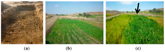
Figure 1.
(a) Photo from the construction of the controlled archaeological environment located at the Alampra village. (b) The area was then cultivated with barley crops. (c) Photo of the barley crop during its full growth. The linear cropmarks formed in the area above the archaeological environment are shown with an arrow (source [32]).
Ground spectroradiometric measurements were made in each campaign, both across the “archaeological” area and the non-archaeological area. A handheld GER 1500 spectroradiometer (Geophysical and Environmental Research Corporation, University of Edinburgh, Scotland) was utilized for this purpose. With 512 distinct channels with a full width at half maximum (FWHM) of around 1.5 nm, this device can record electromagnetic radiation from the visible to near-infrared spectrum (400–1050 nm). Additionally, all of the observations made over the crops were calibrated and the incoming sun radiation was measured using a Lambertian spectralon panel (Geophysical and Environmental Research Corporation, University of Edinburgh, Scotland) [33]. This panel has the capability to reflect the incoming radiation to almost 100% (99.996%) in all directions. The instrument’s field of view (FOV) was adjusted to 4 degrees (≈0.02 m2 from 1.2 m above the ground). The reference measurement at the spectralon Lambertian surface panel was first used to determine the incoming radiance, followed by the subsequent measurements. These steps were repeated during and in each different campaign to harmonize and calibrate the overall spectral signatures. The range of spectral signatures is between 0 and 100%.
Multi-temporal ground spectroradiometric campaigns have been carried out over the simulated test field from October 2011 until April 2012. In particular, there are 16 days of observation, with a varying number of measurements in each day. The number of A and H reflectance observations ρ made on particular dates is given in Table 1. Label A refers to the measurements taken over the simulated “archaeological” subsurface target and Label H refers to the measurements taken over healthy vegetation (crops).

Table 1.
Observations per day.
The overall methodology adopted for the needs of this study is depicted in Figure 2. Once the datasets have been collected, they are quantitatively processed (rescaled to the unit interval and forming the average of the ratio of every signature to any other in the dataset) to facilitated classification. Using machine learning algorithms, specifically decision trees [34], we identify two new (single wavelength) indices and the associated thresholds (decision boundaries), which optimally classify the dataset into healthy and stress vegetation spectral profiles (H and A, respectively). Taking into consideration the noise impact, the new indices and thresholds were produced based on the suitable spectral windows. Finally, the physically based model PROSAIL was used to estimate physical parameters and identify decision boundaries associated with them. This analysis singles out the leaf chlorophyll content as the physical parameter that can be effectively used for classification purposes.
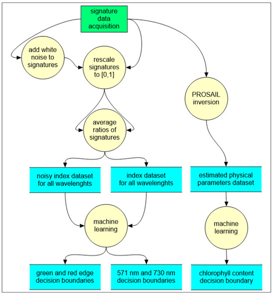
Figure 2.
Overall methodology implemented in this study.
3. Results
The above-mentioned ground spectroradiometric datasets were processed in the Python programming language [35]. The different processing steps and their results are illustrated in the following subsections.
3.1. Analysis of the Dataset and Data Transformation
Our analysis of this dataset proceeds as follows. Consider the measured A reflectance curves of a single day of observation, e.g., 11 February 2012, as shown in Figure 3a. The spectral profile of these curves is characteristic of what we see in healthy vegetation: low reflectance values in the visible part of the spectrum, i.e., approximately between 450 and 630 nm, with a small increase in the green part of the spectrum around 560 nm and a sudden increase in the near-infrared part after 700 nm. Between 630 and 700 nm is the so-called red edge part of the spectrum. Observing these curves, we can see that there is a certain degree of similarity between them, indicating a nearly similar and a difference in scale (i.e., absolute reflectance values).
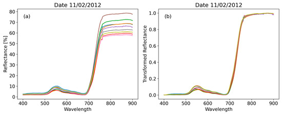
Figure 3.
Measured and transformed A reflectance curves for a given day, indicated with a different colour. (a) Spectral signatures are captured from the spectroradiometer and (b) transformed reflectance curves based on Equation (1).
Therefore, the next step could be to isolate this pattern of the curves. Therefore, we transform (shift and rescale) each curve by linearly mapping the reflectance so that its range becomes [0, 1], i.e., its minimum and maximum are mapped into 0 and 1, respectively, based on Equation (1):
The index i runs over the number of observed curves. The transformed reflectance curves for the given date are shown in Figure 3b.
The effect of this transformation is clear: the relative significance of the differences in pattern, e.g., between the visible spectrum and the red edge, as shown in Figure 3b, is much more pronounced than before (Figure 3a). In contrast, the differences in absolute reflectance values observed in the near-infrared part of the spectrum are not further visible. Our further analysis will be based on the transformed reflectance curves (Figure 3b).
Let us now plot the (transformed) reflectance curves against each other, which we may call reflectance-against-reflectance plots. In Figure 4, for a given day of observation (17 March 2012), the A and H reflectance curves are plotted against each other, in all distinct combinations of A and H in the following manner: in Figure 4a, all H measured curves of the day are plotted against a single H curve, which serves as the horizontal axis. Similarly, for the other two figures (all A against a single H in Figure 4b and all H against a single H curve in Figure 4c.).
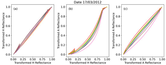
Figure 4.
Reflectance-against-reflectance curves (all combinations) from a date in the JFM period. (a) all H measured curves of the day plotted against a single H curve. (b) all A against a single H curve and (c) all A against a single A curve. Different colours correspond to different measurements on the given data.
One observes a specific pattern in the A against H graph in Figure 4b, i.e., A curve values are depressed relative to the H curve values at the same wavelength. The patterns shown in Figure 4 are characteristic of any given day in the January–February–March (JFM) period, and the A and H curves serve as the horizontal axis, as shown in Figure 4. The period JFM was selected from the overall observation timeframe as this is the period (phenological cycle) where the crops start to grow in the area; therefore, we can observe the spectral signature pattern, as shown in Figure 3a.
On the other hand, if the same analysis is carried out on any observation date in other phenological periods, the result is qualitatively different, as can be seen in Figure 5 for 31 October 2011. During that period, the crops have just been seeded and the spectral signatures thus correspond to those of soil targets rather than crops. Therefore, one realizes that one should focus on the JFM period, which is consistent with the growth stage of barley. The JFM period contains a dataset of 107 observations (reflectance signatures) to work with.
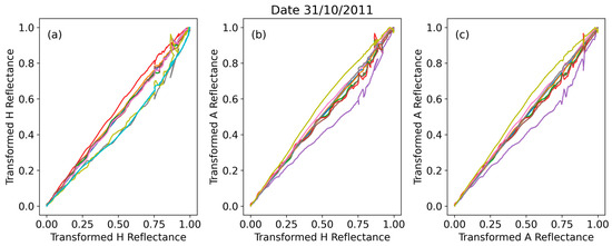
Figure 5.
Reflectance-against-reflectance curves (all combinations) from a date outside the JFM period. (a) all H measured curves of the day plotted against a single H curve. (b) all A against a single H curve and (c) all A against a single A curve. Different colours correspond to different measurements on the given data.
We may momentarily pause to generalize what we have carried out so far, thinking in terms of an unknown dataset of similar spread throughout the months of the year. Let us pretend that the given dataset (spectral signature) is unknown, and in any specific measurement day pick any reflectance curve and set all the others against it, and then perform that for all curves of the day (we always refer to the transformed ones). In Figure 6, we show the results of this process for a date in the JFM period; we have chosen 4 March 2012, for two reflectance curves we called X_1 (unknown #1) and X_2 (unknown #2). It is clear that unknown #1 must be A while unknown #2 must be H. Indeed, Figure 6a indicates a stressed pattern (below the diagonal line 1:1) while, in contrast, in Figure 6b, a healthy crop profile (near and above the diagonal line 1:1) is observed.
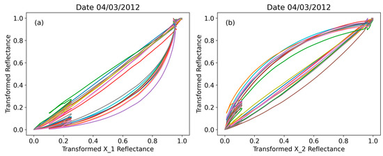
Figure 6.
Analysis of an ‘unknown’ dataset via inspection: Reflectance-against-reflectance curves for observation X_1 against all the observations in the given date. X_1 and X_2 can be identified as (a) A and (b) H, respectively, based on their pattern.
In the reflectance-against-reflectance type of plot, as in the case of Figure 4, Figure 5 and Figure 6, it is not clear which part of the spectrum they mainly visualize. In Figure 7, we plot an A reflectance curve against an H reflectance curve for any specific date in the JFM period (here, we have chosen 4 March 2012). Suitably restricting the range, it is clarified that the main phenomena refer to the red edge part of the spectrum. Anticipating a discussion that will be the subject of Section 3.6, we may observe that the resulting trend, which can be fitted with near perfection with very simple functions, suggests that quite specific physical phenomena are at work here to produce this result.
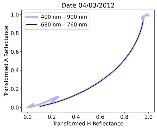
Figure 7.
Reflectance-against-reflectance curves emphasize the red edge part of the spectrum.
3.2. Definition of a (Single-Wavelength) Classifying Index within the Visible Spectrum
The previous discussion suggests that in a dataset of (transformed) reflectance curves, the A reflectance curves have in general smaller ordinates than the H reflectance curves, at least in a part of the spectrum. In order to make such observations general and quantitative, we may form ratios of the reflectance curves using Equation (2):
That is, for the i-th reflectance curve, we obtain N ρ-ratio curves (where N is the size of the original dataset), or more precisely, N-1 non-trivial ones. We may now observe that if the i-th curve is an A reflectance, then its ρ-ratio curves will lie lower that the ρ-ratio curves of an i′-th curve, which is H reflectance. This statement can be made specific by averaging the ρ-ratio curves corresponding to any specific observed reflectance (Equation (3)):
That is, for every wavelength λ, we average ρ-ratios of any reflectance curve relative to any other reflectance curve in the dataset (always referring to the transformed ones). The mean ρ-ratio is essentially an index associated with every signature for all wavelengths. Given our discussion above, the assumption is that there might be a critical value of the mean ρ-ratio, serving as a decision boundary, separating the A from the H reflectance curves (with an acceptably high success rate).
A technical detail that should be taken care of is that the denominator of ratios of normalized reflectances may be zero for certain wavelengths in the visible spectrum (see Figure 3b). This can be achieved by introducing a small cutoff, that is, by clipping all values below that cutoff and setting them to be equal to it. That cutoff should only serve as a facilitator of calculations, that is, its value should not affect the final results if it is small enough. Indeed, it turns out that any cutoff value below 5 × 10⁻⁵ produces the same results.
The mean ρ-ratios for all observed reflectance curves and for all wavelengths are shown in Figure 8. One may then discover by mere inspection that in the vicinity of the peak of the original reflectance curves in the visible spectrum, i.e., near 560 nm, there is very clear separation between the A and H mean ρ-ratios. We should emphasize again that this fact survives for all small values of the cutoff, which primarily affect these curves near the blue and red edges.
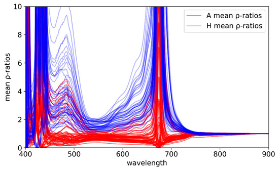
Figure 8.
Mean ρ-ratio curves associated with each observed reflectance curve.
At first, we may proceed empirically. The most promising region is the one around the peak of the reflectance within the visible region (~550 nm). By inspection, one finds that the mean ρ-ratio at (approximately) 570 nm is the most suitable variable to define a decision boundary between the A and H observations. Therefore, we shall define the following index (Equation (4)) as follows:
In Figure 9, we plot this index for all observations. We find that there is indeed a distinctive decision boundary between A and H observations at the value Index570 = 1.2 (rounded to one decimal point).
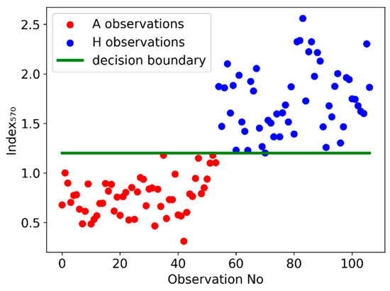
Figure 9.
Index570 for all A and H observations and the decision boundary at 1.2.
To be more precise, if we identify an observation as A if its Index570 is greater than 1.2, then the standard classification scores of this method show no failure (Table 2).
Table 2.
Classification scores for Index570 decision boundary at 1.2.
We may note at this point that score values such as those observed in Table 2 usually imply excessive overfitting. But it is hard to argue for such an interpretation given that the results were obtained with a single degree of freedom. Then, another interpretation might be that the dataset is—in some way—too biased. Indeed, the dataset does not have the complications and deficiencies of satellite imagery, nor it is spread across many different test cases. Simulating a certain level of noise in the measured reflectance signatures adds some realism into the quality of the data, and its effects can be quantified. This is outlined below. Moreover, we could argue that the classification methods discussed here can be directly interpreted in terms of the physical properties of the canopy, thereby adding a certain amount of generality/universality to our results.
3.3. Machine Learning Methods: Analysis with Logistic Regression and Decision Tree Classifiers
Although the 570 nm wavelength and a value of 1.2 for the Index were found in an empirical fashion by inspecting the patterns in Figure 8, we would like to obtain the decision boundary and the associated wavelength(s) in a systematic way, as well to know why that worked given the hundreds of degrees of freedom present in the mean ρ-ratio curve. More importantly, given that real (i.e., satellite observations) data will have a more complex structure than our dataset, it is necessary to look at and understand alternative ways to identify the A observations.
To simplify our analysis, we group the wavelengths between 400 and 900 nm (covering the visible to near-infrared part of the spectrum) into bands of 10 nm averaging the values of the mean ρ-ratio in every band. We use the central points of the bands, i.e., 405, 415,…,895, as the name of the corresponding feature (variable), reducing the number of the features to 50. We first calculate the 50 × 50 correlation matrix of the features, which is visualized in Figure 10.
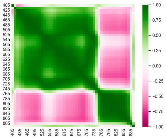
Figure 10.
Correlation matrix of the mean ρ-curves averaged over 10 nm.
We observe that the correlation matrix is nearly block-diagonal, forming two blocks in the visible/red edge and near-infrared parts of the spectrum. The latter in particular forms a block of strongly correlated features. We observe that the wavelengths in the neighborhood of 550 nm are weakly correlated with other wavelengths, except for the wavelengths at the outer part of the red edge. This may be regarded as an explanation for why the Index defined above can carry so much information alone. The wavelengths in the neighborhood of 680 nm as well as 480 nm are negatively correlated with the near-infrared spectrum. In fact, 680 nm wavelengths are quite strongly correlated with a large part of the visible spectrum. Overall, these strong correlations imply that the effective degrees of freedom are much fewer than the number of features.
Let us first model the classification of the curves into A and H through the logistic regression classifiers available in the Python language libraries [35]. Logistic regression involves all degrees of freedom (features) simultaneously finding the relative weight (importance) of them in obtaining the answer. Although the empirical analysis of the problem suggests that regression is not the most suitable method to consider, it is interesting to see how it performs and obtain the pattern regarding the importance of features.
After reshuffling, we split the available datasets of 107 observations into 85 observations (80%) for the training set and 22 (20%) for the validation set. The obtained model performance is again given in Table 2, achieving perfect scores. It should be noted, though, that the 10 nm bands appear to be the coarser resolution producing the best results: with bands of 20 nm, scores are lowered to 96%. The importance of every feature (wavelength), that is, the coefficients of the fitted logistic regression model, is shown in Figure 11.
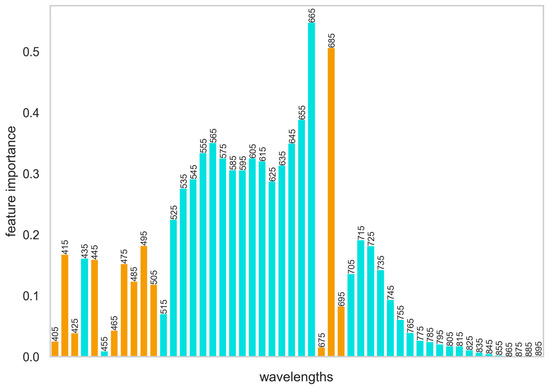
Figure 11.
Feature importance for the logistic regression model. Positive values are given in orange, while negative are given in cyan.
In this method, the classification is described quite differently than the single wavelength Index570. Wavelengths around 660 nm have the greatest relative (positive) importance, while wavelengths around 480 and 680 nm do contribute significantly but counterbalance (by having the opposite sign) the contributions of the majority of the features (appearing in the blocks of the correlation matrix). Also, the wavelengths in the upper block contribute significantly and rather equally.
Decision tree classifiers are more pertinent to the problem at hand, as the method finds decision boundaries examining sequentially its features [34,36]. Moreover, the relatively small size of the dataset and the rather low number of degrees of freedom, as well as the ‘white-box’ interpretability of decision trees [37], make this classification method a suitable approach for the current purpose. Indeed, again constructing a training and validation set and using gini impurity as a measure of the quality of the splits, we find that for a simple depth equal to 1 (one node), there is a decision boundary, a single dominant feature at 571 nm, i.e., the only wavenumber with a non-zero weight and equal to 1 (Figure 12), and a decision boundary (threshold) of 1.191, as shown in Figure 13, where our decision tree is visualized. This is in accordance with our expectations from the analysis that led to the Index570 and the associated decision boundary. The decision tree classification allowed us to validate and refine that analysis, as well as to deduce these results in a systematic way, i.e., through an algorithm instead of inspection.
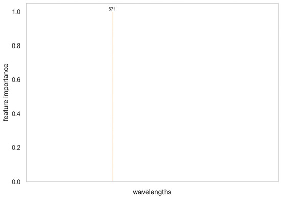
Figure 12.
Feature importance for the decision tree model. A single feature dominates.
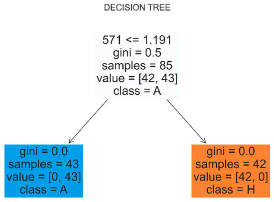
Figure 13.
Visualization of the decision tree.
Upon checking the fitted model on the validation set, we again find the perfect scores given in Table 2.
3.4. Simulating the Effects of Noise: Statistics of the Classifying Index570
At this point, it is necessary to incorporate the presence of noise into our analysis, which is always part of real (e.g., satellite imagery) observations. We simulate adding white (i.e., uncorrelated) noise, drawn from a normal distribution N(μ,σ) with the mean value μ equal to the value ρ of the (original) reflectance signature curve (at any given wavelength λ) and standard deviation σ = CV∗ρ, where CV is the coefficient of variance, which will be fixed at 5%. That is (Equation (5)),
This way, an ensemble of simulations of the dataset may be generated and the previous analyses may be applied for each element (dataset) of the ensemble. In particular, two important analyses may be applied: (1) to investigate the performance of Index570 with decision boundary 1.2, that is, determine the statistics of the classification scores, and (2) to investigate the statistics of the decision boundary as determined by a decision tree.
First, we would like to visualize the mean ρ-curves of the ensemble of A and H observations. These curves are shown in Figure 14 for 100 simulations of the dataset with noise.
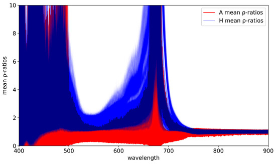
Figure 14.
Mean ρ-curves of an ensemble of simulated observations, totaling 100 × 107 curves.
Once the ensemble of mean ρ-curves for the A and H observations has been constructed, it is straightforward to apply classification methods and evaluate the statistics of the success rate. First, we perform this for the Index570 and deduce the score statistics for the associated classification criterion proposed in this work, i.e., that a reflectance signature is A if its Index570 < 1.2.
The results shown in Table 3 indicate that the classification based on the Index570 performs very well even in the presence of noise; we obtained a success rate of approximately 97% ± 2%. Hence, it might turn out to be an effective tool in actual applications.
Table 3.
Statistics of classification scores for the Index570 < 1.2 criterion.
Our second task is to study these simulations through the decision tree method in order to obtain the statistics of the dominant wavenumber and thresholds. In this case, both the chosen wavelength and the decision boundary will be discovered by the method itself, and they will thus vary. The obtained results will allow us to refine the definition of the Index when dealing with noisy dataset. As mentioned earlier, the decision tree classification has a greater affinity to the Index method proposed in this work and can naturally be regarded as a validation as well as refinement of the latter.
Indeed, in the case of the simulation ensemble, a tree depth equal to 2 was needed in some of the realizations, that is, at most two wavenumbers had a non-zero weight. It should be mentioned that the classification scores on the validation set remain essentially the same from depth 1 to depth 2; hence, we shall proceed with depth 2. As the decision boundary is, in general, a multidimensional boundary surface in the feature space, here, we quote the thresholds at which the tree splits data for the dominant wavelength. For more stable statistical results, we use an ensemble of 5000 simulations. The statistics of the classification scores are given in Table 4, together with the dominant wavelength (with importance ~0.95 or higher) and the associated threshold. Classification scores reach as high as 98%.
Table 4.
Statistics of classification parameters for the decision tree method.
The distribution of the dominant wavelength (frequency of appearance) is presented in Figure 15. On top of every bar is the mean value of the threshold for that wavelength. The wavelength 568 nm is the most frequently arising wavelength of the distribution, but there are other values with significant rates of appearance. Table 5 shows certain important percentiles of the distribution. We see that between the 5th and 95th percentile there are many wavelengths that arise with a significant probability.
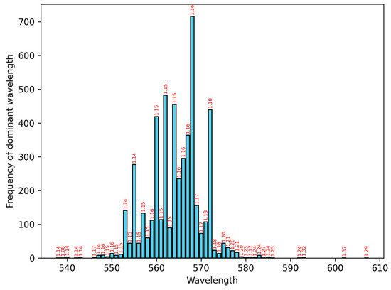
Figure 15.
Histogram of the dominant wavelength values for the 5000 simulations. On top of every bar is the mean value of the threshold for that wavelength.
Table 5.
Percentiles of the dominant wavelength distribution.
Inspection of the threshold values in Figure 15 shows that the threshold values increase with the wavelength in this part of the spectrum. This is shown more concretely in Figure 16, where one may see a very distinct trend in (roughly) the 5–95th percentile interval of the wavelength distribution. Outside this interval, the events in every wavelength are too few; hence, the (plotted) mean value of the threshold fluctuates a lot even over 5000 simulations.
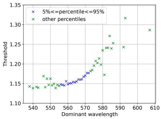
Figure 16.
The average threshold as a function of the corresponding dominant wavelength value for the visible part of the spectrum.
The simple (monotonic) trend shown in Figure 16 facilitates the definition of a classification index for the noisy data and the choice of the decision boundary to form a classification criterion. We may define the index as the average of mean ρ-ratios over the interval containing the representative wavelengths, 555–572 nm. We formalize this in Equation (6):
Then, choosing the decision boundary from the thresholds of the smaller wavelengths (smaller thresholds), we will have great precisions (few false positives) but relatively low recall (low success rate in the identification of positives). If, on the other hand, we choose the decision boundary from the thresholds of the larger wavelengths (larger thresholds) and particularly the value 1.17 corresponding to the 95th percentile of the wavelength distribution, a nice balance between the magnitudes of the classification scores is attained. The very good performance of this criterion is given in Table 6.
Table 6.
Statistics of classification parameters for the Index570 < 1.17 criterion over the ensemble.
3.5. The Red Edge
Our analysis in Section 2 suggests that classification in the red edge part of the spectrum could be carried out, with a high degree of success, by mere visual inspection, at least in the given dataset. We would like to systematize this analysis and, hence, quantify its performance for this observation. We shall perform that by using decision tree classification.
Indeed, applying this method to the mean ρ-ratio curves for 680–760 nm, we find that there is a dominant wavelength (with an importance of 0.91) at 731 nm. Figure 17 provides a visualization of this decision tree. We see that depth 3 is required in the case of the red edge. The threshold of the dominant value comes at 1.065. The obtained model returns classification scores of 1.0 in the validation set. This information is summarized in Table 7.
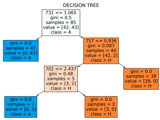
Figure 17.
Visualization of the decision tree classification in the red edge.
Table 7.
Classification parameters for red edge using decision trees.
Next, we investigate the effects of noise applying the same analysis in its element of the ensemble of simulated reflectance signatures. The mean values of the classification scores on the validation set attain a peak for tree depth 3; hence, we stop there, and in what follows, we quote these results. For more stable statistical results, we again use an ensemble of 5000 simulations. The statistics of the performance of the decision tree model are shown in Table 8. The obtained classification scores are ~91%. Overall, one may conclude that using indices in the red edge regime of the spectrum is expected to be less effective than within the visible spectrum.
Table 8.
Statistics of classification parameters for the decision tree method.
The distribution of the dominant wavelength (whose importance is always greater than 0.79) is shown in the histogram in Figure 18. On top of every bar of the histogram is the mean value of the threshold for that wavelength. The wavelength distribution has a mean ± standard deviation at 728 ± 5 nm. The interval 728–731 nm can be regarded as representative. Certain percentiles of the distribution are given in Table 9.
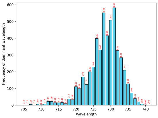
Figure 18.
Histogram of the dominant wavelengths’ values for the 5000 simulations from the red edge. On top of every bar, the mean value of the threshold for that wavelength is shown.
Table 9.
Percentiles of the dominant wavelength distribution.
Thresholds are plotted against the corresponding wavelength in Figure 19. There is again a strong trend, as we also saw in the visible spectrum analysis, only this time decreasing. As before, the trend is less clear outside the 5–95th percentile interval due to fewer events there. The simplicity (monotonicity) of the relationship allows us to easily deal with the tradeoff between precision and recall in the way we define a classification index and choose the decision boundary, as it also occurred in the case of the visible spectrum. Defining the index by the wavelengths of the representative interval and choosing the decision boundary from the thresholds of the larger wavelengths (smaller thresholds), we obtain great precision and relatively low recall. Alternatively, choosing the decision boundary from the thresholds of the smaller wavelengths (larger thresholds), and specifically, the value 1.10 corresponding to the 5th percentile of the wavelength distribution, we again manage to have a nice balance between the classification scores.
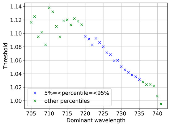
Figure 19.
The trend of the average threshold against the corresponding dominant wavelength value for the red edge part of the spectrum.
Indeed, we define the classification criterion as follows:
The performance of the criterion in Equation (7) is given in Table 10. As expected, this method of classification performs less well than the visible spectrum one; the analogous scores are shown in Table 6.
Table 10.
Statistics of classification parameters for the Index730 < 1.1 criterion over the ensemble.
3.6. Interpretation and Classification on Physically Based Modelling (PROSAIL)
The high correlation between degrees of freedom (wavelengths) we have seen in Figure 10 means that the actual degrees of freedom are actually far fewer than the hundreds of reflectance values in a reflectance signature. The PROSAIL model produces reflectance signatures from about a dozen physical parameters modelling the leaves optical properties and the canopy reflectance properties [38,39]. PROSAIL belongs to a class of radiative transfer models and allows for a physically based retrieval of the plant properties [40,41,42].
In this section, we present a preliminary work relating the physical properties of vegetation and canopy with the A and H classification. We use plausible values and ranges for the PROSAIL input parameters based on the literature [39,41], which are given in Table 11.
Table 11.
The values and ranges of the PROSAIL input parameters used in this study. Parameters with (*) are fitted within the quoted bounds.
Four variables are allowed to vary: Cab, Car, LAI, and lidfa. Inversion is performed using the PROSAIL module [43] and standard optimizers of Python libraries. The statistics of fitting them across the dataset of 107 observations are given in Table 12:
Table 12.
Statistics of fitting the PROSAIL parameters across the dataset of observations.
Scatterplots of the estimated parameters are given in Figure 20, for some of the possible pairs of parameters. As will be further understood shortly, the leaf chlorophyll content Cab is the most important and robust parameter, in the sense of being less sensitive to different choices of parameters than estimated and their assumed bounds (this experimentation cannot be shown here).
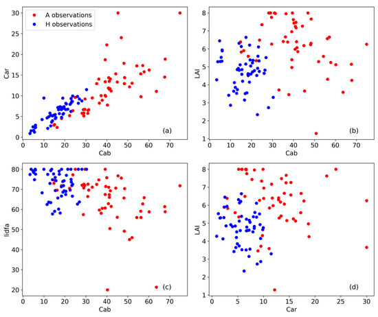
Figure 20.
Scatter plot of the estimated parameters with some of the possible combinations of two: (a) leaf carotenoid content vs leaf chlorophyll content, (b) lead area index vs leaf chlorophyll content, (c) average leaf angle vs leaf chlorophyll content, and (d) leaf area index vs leaf carotenoid content.
The linear relationship between the Car and Cab parameters known in the literature, see, e.g., [44], is verified here, although it was not adopted. The highly important leaf area index (LAI) parameter is estimated to have relatively large values, which is consistent with the growth stage of the plant [41]. The average leaf angle is estimated to be above 40 degrees for all observations and, in fact, above 55 degrees for the A observations. The leaf angle proved to be crucial for good fitting of the reflectance signatures. These observations are consistent with the literature [44].
Inspection of these scatterplots suggests that it is quite meaningful to construct decision boundaries for and A and H classification, that is, to construct the boundary surface in the four-dimensional parameter space. Hence, we next turn to decision trees to provide us with information of that kind.
The four-feature (physical parameters) dataset estimated from the PROSAIL inversion is labeled with A and H and is split randomly with an 80–20 proportionality into training and validation sets. Table 13 shows one of the classification scores (accuracy) on the validation set of the decision tree models built for different depths of the tree. This analysis is necessary to avoid overfitting and hence avoid drawing non-generalizable conclusions from the decision boundary. We see that the scores decrease beyond depth 1, that is, beyond the first split on the dominant variable, which is always the Cab parameter. As we proceed deeper, the scores do not always change, but the relative importance of the parameters does change (not quoted here). The importance of Cab is larger than 78% in all cases. This result means that the construction of a non-trivial boundary surface requires (1) a larger dataset and/or (2) more detailed work on the physical parameter constraints (e.g., regarding season or interdependence) that lies beyond the scope of the present work.
Table 13.
Statistics of accuracy on the validation set for different tree depths.
Hence, physically based classification is expressed in terms of a one-dimensional decision boundary for the chlorophyll content Cab parameter. That boundary (the threshold value for the split) is found to be 28 at two significant figures (Figure 21): if the chlorophyll content of an observed signature is predicted to be lower than 28, then the observation is classified as H, otherwise, it is classified as A.
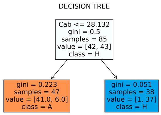
Figure 21.
Depth 1 decision tree for the physical parameter classification.
We formalize this statement by introducing a physical index that is equal to the chlorophyll content in the usual units (μg cm−2). Then, an observation is classified as A if
Let us then run this criterion directly over the dataset of the estimated values of the Cab parameter. Table 14 summarizes the scores found. This index is not as effective as Index570, but it does have a high enough success rate.
Table 14.
Classification scores for Index_phys with decision boundary at 28.1.
Having understood the importance of the Cab parameter, we are in a position to trace the origin of the nearly mathematically perfect pattern observed in the (rescaled) reflectance-against-reflectance curves, deduced from the observed reflectance signatures in, e.g., Figure 6 and Figure 7. To this end, we plot a (rescaled) reflectance-against-reflectance curve derived from PROSAIL, keeping all parameters the same, except Cab, for which the larger value is put on the y-axis, as shown in Figure 22. The result is the pattern we have noticed in the observed curves in Figure 6 and Figure 7.
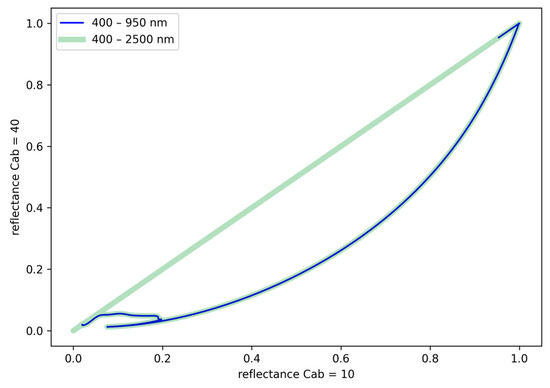
Figure 22.
PROSAIL reflectance-against-reflectance curves for different Cab values.
4. Discussion
The results obtained here provide some interesting insights regarding the optimum wavelength for the detection of cropmarks.
The main findings of this work can be summarized as follows:
- Classification is greatly facilitated by normalizing (rescaling) the calibrated reflectance signatures to the unit interval.
- Reflectance-to-reflectance plots between pairs of rescaled signatures offer a visual means to identify (with great but not absolute success) the stressed signatures in the red edge part of the spectrum.
- Two very effective spectral indices (Index570 and Index730) can be defined in a small band of wavelengths at around 570 and 730 nm, respectively, by dividing the rescaled reflectance of its observation with that of any other observation in the dataset and averaging the result per wavelength and per band. The classification criteria for stress signatures correspond to the indices being less than 1.2 and 1.1, respectively. The indices operate independently, and the visible spectrum index is more effective than the red edge one.
- The indices and criteria are found algorithmically using decision tree classification methods.
- The effect of noise in the observed signatures is taken into account by simulating noise-affected signatures. By deducing and analyzing distributions of the dominant wavelength (Index) and classification thresholds using decision tree methods, we are able to formulate the previously defined indices and criteria for noisy signatures. The proposed methods are shown to be robust with classification scores always greater than 90%.
- An index based on the physical properties of the leaf and canopy (Indexphys) is introduced by analyzing the estimated parameters of the PROSAIL model obtained from the observed signatures by inversion. We find that the leaf chlorophyll content Cab is the dominant classification parameter. For the specific (barley) crop under study, we find that stressed signatures tend to have Cab values greater than 28 μg cm−2 (with an over 90% success rate).
It should be noted that the spectral indices are expected to be more robust than the physically based one, as the former indices are dimensionless and the associated criteria quantify the tendency of the stressed crop signatures to be smaller than the healthy crop signatures.
The absence of the near-infrared part of the spectrum in the abovementioned indices (excluding the red-edge-related index provided in Equation (7)), which is usually used for the detection of cropmarks, e.g., through the use of the Normalized Difference Vegetation Index (NDVI), should be linked directly to the proposed methodology and overall analysis carried out here, i.e., by normalizing the reflectance curves, the obvious absolute differences between the spectral signatures observed in the near-infrared part of the spectrum (see Figure 3a) are now minimized (see Figure 3b). Nonetheless, the near-infrared part is involved in the definition of the indices, given that it is used in the rescaling of signatures, given by Equation (1), as the part of the spectrum where the maximum of the signatures occurs.
5. Conclusions
This study introduces and analyzes classification indices and criteria (two spectral and one physical index) of the spectral signatures taken during a complete phenological cycle over crops, in a controlled environment. This environment was constructed to simulate cultivate areas with shallow buried archaeological remains. The main findings of this work were summarized and discussed above.
It is important to highlight that the findings from the presented analysis of the cropmarks using physically based models such as those of PROSAIL can be considered quite novel. To the best of the authors’ knowledge, this is the first study ever to attempt to model stressed vegetation due to the presence of buried archaeological remains with physical properties and modelling. The overall results are quite interesting as the model depicts the most significant parameters that affect the formation of cropmarks in the specific area, and especially the Cab. One may argue that the soil-associated parameters are less significant as the areas compared between H and A measurements were in very close proximity. Even though these findings can be considered peculiar, i.e., for the specific soil context, similar studies in other environments might reveal potential comparisons.
The novel indices proposed in this study are targeted for hyperspectral data. Nevertheless, it should be noted that such hyperspectral data beyond ground spectroradiometers used in the study are quite rare with lower spatial resolution. In contrast, there is a plethora of multispectral satellite, aerial and low-altitude sensors that are widely used for archaeological purposes. Therefore, future directions could be to downscale the results moving from hyperspectral to multispectral bands, which might have a more practical meaning for studying archaeological areas. Additionally, systematic theoretical analysis of observations from different controlled environments, e.g., different locations, crops, methods of cultivation, etc., is required, to establish methods that allow us to analyze real-world applications and archaeological areas.
Author Contributions
Conceptualization, A.A. and E.G.; methodology, A.A. and E.G.; data curation, A.A. and E.G.; writing—original draft preparation, A.A. and E.G.; writing—review and editing, A.A. and E.G.; visualization, A.A. and E.G. All authors have read and agreed to the published version of the manuscript.
Funding
This project has received funding from the European Union’s Horizon Europe Framework Programme (HORIZON-WIDERA-2021-ACCESS-03, Twinning Call) under grant agreement no. 101079377 and the UKRI under project number 10050486.
Data Availability Statement
No new data were created or analyzed in this study. Data sharing is not applicable to this article.
Acknowledgments
Thanks are given to the Remote Sensing Laboratory, Department of Civil Engineering and Geomatics at the Cyprus University of Technology for the support during the collection of the in situ measurements (between 2011 and 2012), as part of the first author’s (A.A) PhD studies.
Conflicts of Interest
The authors declare no conflicts of interest. Views and opinions expressed are, however, those of the authors only and do not necessarily reflect those of the European Union or the UKRI. Neither the European Union nor the UKRI can be held responsible for them.
References
- Luo, L.; Wang, X.; Guo, H.; Lasaponara, R.; Zong, X.; Masini, N.; Wang, G.; Shi, P.; Khatteli, H.; Chen, F.; et al. Airborne and spaceborne remote sensing for archaeological and cultural heritage applications: A review of the century (1907–2017). Remote Sens. Environ. 2019, 232, 111280. [Google Scholar] [CrossRef]
- Agapiou, A.; Lysandrou, V. Remote sensing archaeology: Tracking and mapping evolution in European scientific literature from 1999 to 2015. J. Archaeol. Sci. 2015, 4, 192–200. [Google Scholar] [CrossRef]
- Opitz, R.; Herrmann, J. Recent Trends and Long-standing Problems in Archaeological Remote Sensing. J. Comput. Appl. Archaeol. 2018, 1, 19–41. [Google Scholar] [CrossRef]
- Noviello, M.; Ciminale, M.; De Pasquale, V. Combined Application of Pansharpening and Enhancement Methods to Improve Archaeological Cropmark Visibility and Identification in QuickBird Imagery: Two Case Studies from Apulia, Southern Italy. J. Archaeol. Sci. 2013, 40, 3604–3613. [Google Scholar] [CrossRef]
- Cozzolino, M.; Longo, F.; Pizzano, N.; Rizzo, M.L.; Voza, O.; Amato, V. A Multidisciplinary Approach to the Study of the Temple of Athena in Poseidonia-Paestum (Southern Italy): New Geomorphological, Geophysical and Archaeological Data. Geosciences 2019, 9, 324. [Google Scholar] [CrossRef]
- Kalayci, T.; Simon, F.X.; Sarris, A. A manifold approach for the investigation of Early and Middle Neolithic settlements in Thessaly, Greece. Geosciences 2017, 7, 79. [Google Scholar] [CrossRef]
- Campana, S. Emptyscapes: Filling an ‘empty’Mediterranean landscape at Rusellae, Italy. Antiquity 2017, 91, 1223–1240. [Google Scholar] [CrossRef]
- Saey, T.; Van Meirvenne, M.; De Smedt, P.; Neubauer, W.; Trinks, I.; Verhoeven, G.; Seren, S. Integrating multi-receiver electromagnetic induction measurements into the interpretation of the soil landscape around the school of gladiators at Carnuntum. Eur. J. Soil Sci. 2013, 64, 716–727. [Google Scholar] [CrossRef]
- Masini, N.; Capozzoli, L.; Chen, P.; Chen, F.; Romano, G.; Lu, P.; Tang, P.; Sileo, M.; Ge, Q.; Lasaponara, R. Towards an operational use of geophysics for archaeology in Henan (China): Methodological approach and results in Kaifeng. Remote Sens. 2017, 9, 809. [Google Scholar] [CrossRef]
- Donati, J.C.; Sarris, A.; Papadopoulos, N.; Kalaycı, T.; Simon, F.X.; Manataki, M.; Moffat, I.; Cuenca-García, C. A regional approach to ancient urban studies in Greece through multi-settlement geophysical survey. J. Field Archaeol. 2017, 42, 450–467. [Google Scholar] [CrossRef]
- Doneus, M.; Briese, C. Airborne Laser Scanning in forested areas–potential and limitations of an archaeological prospection technique. Remote Sens. Archaeol. Herit. Manag. 2011, 3, 59–76. [Google Scholar]
- Sarris, A.; Papadopoulos, N.; Agapiou, A.; Salvi, M.C.; Hadjimitsis, D.G.; Parkinson, W.A.; Yerkes, R.W.; Gyucha, A.; Duffy, P.R. Integration of geophysical surveys, ground hyperspectral measurements, aerial and satellite imagery for archaeological prospection of prehistoric sites: The case study of Vésztő-Mágor Tell, Hungary. J. Archaeol. Sci. 2013, 40, 1454–1470. [Google Scholar] [CrossRef]
- Brivio, P.A.; Pepe, M.; Tomasoni, R. Multispectral and multiscale remote sensing data for archaeological prospecting in an alpine alluvial plain. J. Cult. Herit. 2000, 1, 155–164. [Google Scholar] [CrossRef]
- Lasaponara, R.; Masini, N. Detection of archaeological crop marks by using satellite Quick Bird multispectral imagery. J. Archaeol. Sci. 2007, 34, 214–221. [Google Scholar] [CrossRef]
- Rajani, M.B.; Rajawat, A.S. Potential of satellite-based sensors for studying distribution of archaeological sites along palaeochannels: Harappan sites a case study. J. Archaeol. Sci. 2011, 38, 2010–2016. [Google Scholar] [CrossRef]
- Lasaponara, R.; Masini, N. Beyond modern landscape features: New insights in the archaeological area of Tiwanaku in Bolivia from satellite data. Int. J. Appl. Earth Obs. Geoinform. 2014, 26, 464–471. [Google Scholar] [CrossRef]
- Orengo, H.; Petrie, C. Large-Scale, Multi-Temporal Remote Sensing of Palaeo-River Networks: A Case Study from Northwest India and its Implications for the Indus Civilisation. Remote Sens. 2017, 9, 735. [Google Scholar] [CrossRef]
- Agapiou, A.; Alexakis, D.D.; Sarris, A.; Hadjimitsis, D.G. Evaluating the Potentials of Sentinel-2 for Archaeological Perspective. Remote Sens. 2014, 6, 2176–2194. [Google Scholar] [CrossRef]
- Šošić Klindžić, R.; Šiljeg, B.; Kalafatić, H. Multiscale and Multitemporal Remote Sensing for Neolithic Settlement Detection and Protection—The Case of Gorjani, Croatia. Remote Sens. 2024, 16, 736. [Google Scholar] [CrossRef]
- Verhoeven, G.J. Near-Infrared Aerial Crop Mark Archaeology: From Its Historical Use to Current Digital Implementations. J. Archaeol. Method Theory 2012, 19, 132–160. [Google Scholar] [CrossRef]
- Czajlik, Z.; Árvai, M.; Mészáros, J.; Nagy, B.; Rupnik, L.; Pásztor, L. Cropmarks in aerial archaeology: New Lessons from an Old Story. Remote Sens. 2021, 13, 1126. [Google Scholar] [CrossRef]
- Agapiou, A.; Hegyi, A.; Gogâltan, F.; Stavilă, A.; Sava, V.; Sarris, A.; Floca, C.; Dorogostaisky, L. Exploring the largest known Bronze Age earthworks in Europe through medium resolution multispectral satellite images. Int. J. Appl. Earth Obs. Geoinf. 2023, 118, 103239. [Google Scholar] [CrossRef]
- Ruciński, D.; Rączkowski, W.; Niedzielko, J. A Polish perspective on optical satellite data and methods for archaeological sites prospection. In Proceedings of the Third International Conference on Remote Sensing and Geoinformation of the Environment (RSCy2015), Paphos, Cyprus, 16–19 March 2015; Volume 9535, pp. 258–265. [Google Scholar]
- Bini, M.; Isola, I.; Zanchetta, G.; Ribolini, A.; Ciampalini, A.; Baneschi, I.; Mele, D.; D’Agata, A.L. Identification of leveled archeological mounds (Höyük) in the alluvial plain of the Ceyhan River (Southern Turkey) by satellite remote-sensing analyses. Remote Sens. 2018, 10, 241. [Google Scholar] [CrossRef]
- Schneidhofer, P.; Tonning, C.; Cannell, R.J.; Nau, E.; Hinterleitner, A.; Verhoeven, G.J.; Gustavsen, L.; Paasche, K.; Neubauer, W.; Gansum, T. The influence of environmental factors on the quality of GPR data: The Borre Monitoring Project. Remote Sens. 2022, 14, 3289. [Google Scholar] [CrossRef]
- Cowley, D.C. Creating the cropmark archaeological record in East Lothian, southeast Scotland. In Prehistory without Borders: Prehistoric Archaeology of the Tyne-Forth Region; Oxbow: Oxford, UK, 2016; pp. 59–70. [Google Scholar]
- Agapiou, A.; Hadjimitsis, D.G.; Sarris, A.; Georgopoulos, A.; Alexakis, D.D. Optimum temporal and spectral window for monitoring crop marks over archaeological remains in the Mediterranean region. J. Archaeol. Sci. 2013, 40, 1479–1492. [Google Scholar] [CrossRef]
- Aqdus, S.A.; Drummond, J.; Hanson, S.W. Discovering archaeological cropmarks: A hyperspectral approach. Int. Arch. Photogramm. Remote Sens. Spat. Inf. Sci. 2008, 37, 361–365. [Google Scholar]
- Aqdus, S.A.; Hanson, S.W.; Drummond, J. The potential of hyperspectral and multi-spectral imagery to enhance archaeological cropmark detection: A comparative study. J. Archaeol. Sci. 2012, 39, 1915–1924. [Google Scholar] [CrossRef]
- Masini, N.; Marzo, C.; Manzari, P.; Belmonte, A.; Sabia, C.; Lasaponara, R. On the characterization of temporal and spatial patterns of archaeological crop-marks. J. Cult. Herit. 2018, 32, 124–132. [Google Scholar] [CrossRef]
- Agapiou, A. Development of a Novel Methodology for the Detection of Buried Archaeological Remains Using Remote Sensing Techniques. Ph.D. Thesis, Cyprus University of Technology, Limassol, Cyprus, 2013, (unpublished). Available online: https://hdl.handle.net/20.500.14279/877 (accessed on 8 May 2024).
- Agapiou, A.; Hadjimitsis, D.G.; Alexakis, D.D. Evaluation of Broadband and Narrowband Vegetation Indices for the Identification of Archaeological Crop Marks. Remote Sens. 2012, 4, 3892–3919. [Google Scholar] [CrossRef]
- Geophysical and Environmental Research Corporation. Available online: https://fsf.nerc.ac.uk/instruments/ger1500.shtml (accessed on 27 April 2024).
- Kotsiantis, S.B. Decision trees: A recent overview. Artif. Intell. Rev. 2013, 39, 261–283. [Google Scholar] [CrossRef]
- Python Programming Language. Available online: https://www.python.org/ (accessed on 14 March 2024).
- Géron, A. Hands-on Machine Learning with Scikit-Learn, Keras, and TensorFlow; O’Reilly Media Inc.: Sebastopol, CA, USA, 2022. [Google Scholar]
- Linardatos, P.; Papastefanopoulos, V.; Kotsiantis, S. Explainable AI: A review of machine learning interpretability methods. Entropy 2020, 23, 18. [Google Scholar] [CrossRef]
- Féret, J.B.; Gitelson, A.A.; Noble, S.D.; Jacquemoud, S. PROSPECT-D: Towards modeling leaf optical properties through a complete lifecycle. Remote Sens. Environ. 2017, 193, 204–215. [Google Scholar] [CrossRef]
- Berger, K.; Atzberger, C.; Danner, M.; D’Urso, G.; Mauser, W.; Vuolo, F.; Hank, T. Evaluation of the PROSAIL model capabilities for future hyperspectral model environments: A review study. Remote Sens. 2018, 10, 85. [Google Scholar] [CrossRef]
- Duan, S.B.; Li, Z.L.; Wu, H.; Tang, B.H.; Ma, L.; Zhao, E.; Li, C. Inversion of the PROSAIL model to estimate leaf area index of maize, potato, and sunflower fields from unmanned aerial vehicle hyperspectral data. Int. J. Appl. Earth Obs. Geoinform. 2014, 26, 12–20. [Google Scholar] [CrossRef]
- Li, Z.; Jin, X.; Yang, G.; Drummond, J.; Yang, H.; Clark, B.; Zhao, C. Remote sensing of leaf and canopy nitrogen status in winter wheat (Triticum aestivum L.) based on N-PROSAIL model. Remote Sens. 2018, 10, 1463. [Google Scholar] [CrossRef]
- Berger, K.; Verrelst, J.; Féret, J.B.; Wang, Z.; Wocher, M.; Strathmann, M.; Hank, T. Crop nitrogen monitoring: Recent progress and principal developments in the context of imaging spectroscopy missions. Remote Sens. Environ. 2020, 242, 111758. [Google Scholar] [CrossRef] [PubMed]
- Sinha, S.K.; Padalia, H.; Dasgupta, A.; Verrelst, J.; Rivera, J.P. Estimation of leaf area index using PROSAIL based LUT inversion, MLRA-GPR and empirical models: Case study of tropical deciduous forest plantation, North India. Int. J. Appl. Earth Obs. Geoinform. 2020, 86, 102027. [Google Scholar] [CrossRef]
- Danner, M.; Berger, K.; Wocher, M.; Mauser, W.; Hank, T. Fitted PROSAIL parameterization of leaf inclinations, water content and brown pigment content for winter wheat and maize canopies. Remote Sens. 2019, 11, 1150. [Google Scholar] [CrossRef]
Disclaimer/Publisher’s Note: The statements, opinions and data contained in all publications are solely those of the individual author(s) and contributor(s) and not of MDPI and/or the editor(s). MDPI and/or the editor(s) disclaim responsibility for any injury to people or property resulting from any ideas, methods, instructions or products referred to in the content. |
© 2024 by the authors. Licensee MDPI, Basel, Switzerland. This article is an open access article distributed under the terms and conditions of the Creative Commons Attribution (CC BY) license (https://creativecommons.org/licenses/by/4.0/).