
Tracking Water Quality and Macrophyte Changes in Lake Trasimeno (Italy) from Spaceborne Hyperspectral Imagery
 , , , ,
  and
and
Abstract
:1. Introduction
2. Data and Methods
2.1. Study Area
2.2. Data Collection
2.2.1. In Situ Data
2.2.2. Spaceborne Data

| PRISMA | DESIS | EnMAP | |
|---|---|---|---|
| Launch | 22 March 2019 | 29 June 2018 | 1 April 2022 |
| Coverage | 70°N to 70°S | 55°N to 52°S | Global in near-nadir mode |
| Ground sampling distance | HYP: 30 m; PAN: 5 m | 30 m | 30 m |
| Number of bands | HYP: 240 [400–2500 nm] PAN: 1 [400–700 nm] | 235 (no binning) 60 (binning) [400–1000 nm] | 246 [420–2450 nm] |
| Radiometric resolution | 12 bits | 13 bits + 1 bit gain | ≥14 bits |
| Atmospheric correction | MODTRAN v 6.0 (land based) | PACO (land) | PACO (land) MIP (water) |
2.3. Methodology Process Flowchart
2.4. Image Pre-Processing
2.5. Algorithms for Aquatic Ecosystem Mapping
2.5.1. BOMBER
2.5.2. Mixture Density Network
2.6. Product Validation
2.7. Spatio-Temporal Analysis
3. Results
3.1. Radiometric Validation
3.2. Water Quality Product Generation and Validation

3.3. Spatio-Temporal Analysis
4. Discussion
5. Conclusions
Author Contributions
Funding
Data Availability Statement
Acknowledgments
Conflicts of Interest
References
- Adrian, R.; O’Reilly, C.M.; Zagarese, H.; Baines, S.B.; Hessen, D.O.; Keller, W.; Livingstone, D.M.; Sommaruga, R.; Straile, D.; Van Donk, E.; et al. Lakes as Sentinels of Climate Change. Limnol. Oceanogr. 2009, 54, 2283–2297. [Google Scholar] [CrossRef] [PubMed]
- Rose, K.C.; Bierwagen, B.; Bridgham, S.D.; Carlisle, D.M.; Hawkins, C.P.; Poff, N.L.; Read, J.S.; Rohr, J.R.; Saros, J.E.; Williamson, C.E. Indicators of the Effects of Climate Change on Freshwater Ecosystems. Clim. Chang. 2023, 176, 23. [Google Scholar] [CrossRef]
- Chapman, D.V.; Sullivan, T. The Role of Water Quality Monitoring in the Sustainable Use of Ambient Waters. One Earth 2022, 5, 132–137. [Google Scholar] [CrossRef]
- Carvalho, L.; Mackay, E.B.; Cardoso, A.C.; Baattrup-Pedersen, A.; Birk, S.; Blackstock, K.L.; Borics, G.; Borja, A.; Feld, C.K.; Ferreira, M.T.; et al. Protecting and Restoring Europe’s Waters: An Analysis of the Future Development Needs of the Water Framework Directive. Sci. Total Environ. 2019, 658, 1228–1238. [Google Scholar] [CrossRef] [PubMed]
- Alikas, K.; Kangro, K.; Randoja, R.; Philipson, P.; Asuküll, E.; Pisek, J.; Reinart, A. Satellite-Based Products for Monitoring Optically Complex Inland Waters in Support of EU Water Framework Directive. Int. J. Remote Sens. 2015, 36, 4446–4468. [Google Scholar] [CrossRef]
- European Commission Water Framework Directive. Available online: https://environment.ec.europa.eu/topics/water/water-framework-directive_en (accessed on 5 March 2024).
- Kratzer, S.; Harvey, E.T.; Canuti, E. International Intercomparison of In Situ Chlorophyll-a Measurements for Data Quality Assurance of the Swedish Monitoring Program. Front. Remote Sens. 2022, 3, 866712. [Google Scholar] [CrossRef]
- Zhai, M.; Zhou, X.; Tao, Z.; Lv, T.; Zhang, H.; Li, R.; Huang, Y. Retrieve of Total Suspended Matter in Typical Lakes in China Based on Broad Bandwidth Satellite Data: Random Forest Model with Forel-Ule Index. Front. Environ. Sci. 2023, 11, 1132346. [Google Scholar] [CrossRef]
- Wen, Z.; Wang, Q.; Ma, Y.; Jacinthe, P.A.; Liu, G.; Li, S.; Shang, Y.; Tao, H.; Fang, C.; Lyu, L.; et al. Remote Estimates of Suspended Particulate Matter in Global Lakes Using Machine Learning Models. Int. Soil Water Conserv. Res. 2024, 12, 200–216. [Google Scholar] [CrossRef]
- Lyu, L.; Song, K.; Wen, Z.; Liu, G.; Fang, C.; Shang, Y.; Li, S.; Tao, H.; Wang, X.; Li, Y.; et al. Remote Estimation of Phycocyanin Concentration in Inland Waters Based on Optical Classification. Sci. Total Environ. 2023, 899, 166363. [Google Scholar] [CrossRef] [PubMed]
- Cazzaniga, I.; Zibordi, G.; Mélin, F. Spectral Features of Ocean Colour Radiometric Products in the Presence of Cyanobacteria Blooms in the Baltic Sea. Remote Sens. Environ. 2023, 287, 113464. [Google Scholar] [CrossRef]
- Roelfsema, C.; Dennison, B.; Phinn, S.; Dekker, A.; Brando, V. Remote Sensing of a Cyanobacterial Bloom (Lyngbya majuscula) in Moreton Bay, Australia. In Proceedings of the IGARSS 2001. Scanning the Present and Resolving the Future. Proceedings. IEEE 2001 International Geoscience and Remote Sensing Symposium (Cat. No.01CH37217), Sydney, Ausralia, 9–13 July 2001; pp. 613–615. [Google Scholar]
- Jeppesen, E.; Peder Jensen, J.; Søndergaard, M.; Lauridsen, T.; Junge Pedersen, L.; Jensen, L. Top-down Control in Freshwater Lakes: The Role of Nutrient State, Submerged Macrophytes and Water Depth. In Shallow Lakes ’95; Springer: Dordrecht, The Netherlands, 1997; pp. 151–164. [Google Scholar]
- Piaser, E.; Berton, A.; Bolpagni, R.; Caccia, M.; Castellani, M.B.; Coppi, A.; Vecchia, A.D.; Gallivanone, F.; Sona, G.; Villa, P. Impact of Radiometric Variability on Ultra-High Resolution Hyperspectral Imagery Over Aquatic Vegetation: Preliminary Results. IEEE J. Sel. Top. Appl. Earth Obs. Remote Sens. 2023, 16, 5935–5950. [Google Scholar] [CrossRef]
- Liang, S.; Gong, Z.; Wang, Y.; Zhao, J.; Zhao, W. Accurate Monitoring of Submerged Aquatic Vegetation in a Macrophytic Lake Using Time-Series Sentinel-2 Images. Remote Sens. 2022, 14, 640. [Google Scholar] [CrossRef]
- Carr, J.; D’Odorico, P.; McGlathery, K.; Wiberg, P. Stability and Bistability of Seagrass Ecosystems in Shallow Coastal Lagoons: Role of Feedbacks with Sediment Resuspension and Light Attenuation. J. Geophys. Res. Biogeosci. 2010, 115, G3. [Google Scholar] [CrossRef]
- Adjovu, G.E.; Stephen, H.; James, D.; Ahmad, S. Overview of the Application of Remote Sensing in Effective Monitoring of Water Quality Parameters. Remote Sens. 2023, 15, 1938. [Google Scholar] [CrossRef]
- Cao, Q.; Yu, G.; Qiao, Z. Application and Recent Progress of Inland Water Monitoring Using Remote Sensing Techniques. Environ. Monit. Assess. 2023, 195, 125. [Google Scholar] [CrossRef] [PubMed]
- Odermatt, D.; Gitelson, A.; Brando, V.E.; Schaepman, M. Review of Constituent Retrieval in Optically Deep and Complex Waters from Satellite Imagery. Remote Sens. Environ. 2012, 118, 116–126. [Google Scholar] [CrossRef]
- Tyler, A.N.; Hunter, P.D.; Spyrakos, E.; Groom, S.; Constantinescu, A.M.; Kitchen, J. Developments in Earth Observation for the Assessment and Monitoring of Inland, Transitional, Coastal and Shelf-Sea Waters. Sci. Total Environ. 2016, 572, 1307–1321. [Google Scholar] [CrossRef] [PubMed]
- Birk, S.; Ecke, F. The Potential of Remote Sensing in Ecological Status Assessment of Coloured Lakes Using Aquatic Plants. Ecol. Indic. 2014, 46, 398–406. [Google Scholar] [CrossRef]
- Phinn, S.; Roelfsema, C.; Dekker, A.; Brando, V.; Anstee, J. Mapping Seagrass Species, Cover and Biomass in Shallow Waters: An Assessment of Satellite Multi-Spectral and Airborne Hyper-Spectral Imaging Systems in Moreton Bay (Australia). Remote Sens. Environ. 2008, 112, 3413–3425. [Google Scholar] [CrossRef]
- Topp, S.N.; Pavelsky, T.M.; Jensen, D.; Simard, M.; Ross, M.R.V. Research Trends in the Use of Remote Sensing for Inland Water Quality Science: Moving Towards Multidisciplinary Applications. Water 2020, 12, 169. [Google Scholar] [CrossRef]
- Samarinas, N.; Spiliotopoulos, M.; Tziolas, N.; Loukas, A. Synergistic Use of Earth Observation Driven Techniques to Support the Implementation of Water Framework Directive in Europe: A Review. Remote Sens. 2023, 15, 1983. [Google Scholar] [CrossRef]
- Rast, M.; Painter, T.H. Earth Observation Imaging Spectroscopy for Terrestrial Systems: An Overview of Its History, Techniques, and Applications of Its Missions. Surv. Geophys. 2019, 40, 303–331. [Google Scholar] [CrossRef]
- Dey, J.; Vijay, R. A Critical and Intensive Review on Assessment of Water Quality Parameters through Geospatial Techniques. Environ. Sci. Pollut. Res. 2021, 28, 41612–41626. [Google Scholar] [CrossRef] [PubMed]
- Leiper, I.; Phinn, S.; Roelfsema, C.; Joyce, K.; Dekker, A. Mapping Coral Reef Benthos, Substrates, and Bathymetry, Using Compact Airborne Spectrographic Imager (CASI) Data. Remote Sens. 2014, 6, 6423–6445. [Google Scholar] [CrossRef]
- Vahtmäe, E.; Paavel, B.; Kutser, T. How Much Benthic Information Can Be Retrieved with Hyperspectral Sensor from the Optically Complex Coastal Waters? J. Appl. Remote Sens. 2020, 14, 1. [Google Scholar] [CrossRef]
- Turpie, K.R.; Klemas, V.V.; Byrd, K.; Kelly, M.; Jo, Y.-H. Prospective HyspIRI Global Observations of Tidal Wetlands. Remote Sens. Environ. 2015, 167, 206–217. [Google Scholar] [CrossRef]
- Chander, S.; Pompapathi, V.; Gujrati, A.; Singh, R.P.; Chaplot, N.; Patel, U.D. GROWTH OF INVASIVE AQUATIC MACROPHYTES OVER TAPI RIVER. Int. Arch. Photogramm. Remote Sens. Spat. Inf. Sci. 2018, XLII–5, 829–833. [Google Scholar] [CrossRef]
- Giardino, C.; Bresciani, M.; Valentini, E.; Gasperini, L.; Bolpagni, R.; Brando, V.E. Airborne Hyperspectral Data to Assess Suspended Particulate Matter and Aquatic Vegetation in a Shallow and Turbid Lake. Remote Sens. Environ. 2015, 157, 48–57. [Google Scholar] [CrossRef]
- Adam, E.; Mutanga, O.; Rugege, D. Multispectral and Hyperspectral Remote Sensing for Identification and Mapping of Wetland Vegetation: A Review. Wetl. Ecol. Manag. 2010, 18, 281–296. [Google Scholar] [CrossRef]
- Bresciani, M.; Giardino, C.; Fabbretto, A.; Pellegrino, A.; Mangano, S.; Free, G.; Pinardi, M. Application of New Hyperspectral Sensors in the Remote Sensing of Aquatic Ecosystem Health: Exploiting PRISMA and DESIS for Four Italian Lakes. Resources 2022, 11, 8. [Google Scholar] [CrossRef]
- Niroumand-Jadidi, M.; Bovolo, F.; Bruzzone, L. Water Quality Retrieval from PRISMA Hyperspectral Images: First Experience in a Turbid Lake and Comparison with Sentinel-2. Remote Sens. 2020, 12, 3984. [Google Scholar] [CrossRef]
- Soppa, M.A.; Dinh, D.A.; Silva, B.; Steinmetz, F.; Alvarado, L.; Bracher, A. INTERCOMPARISON OF DESIS, SENTINEL-2 (MSI) AND SENTINEL-3 (OLCI) DATA FOR WATER COLOUR APPLICATIONS. Int. Arch. Photogramm. Remote Sens. Spat. Inf. Sci. 2022, XLVI-1/W1-2021, 69–72. [Google Scholar] [CrossRef]
- Katlane, R.; Doxaran, D.; ElKilani, B.; Trabelsi, C. Remote Sensing of Turbidity in Optically Shallow Waters Using Sentinel-2 MSI and PRISMA Satellite Data. PFG—J. Photogramm. Remote Sens. Geoinf. Sci. 2023, 1–17. [Google Scholar] [CrossRef]
- O’Shea, R.E.; Pahlevan, N.; Smith, B.; Bresciani, M.; Egerton, T.; Giardino, C.; Li, L.; Moore, T.; Ruiz-Verdu, A.; Ruberg, S.; et al. Advancing Cyanobacteria Biomass Estimation from Hyperspectral Observations: Demonstrations with HICO and PRISMA Imagery. Remote Sens. Environ. 2021, 266, 112693. [Google Scholar] [CrossRef]
- Taggio, N.; Aiello, A.; Ceriola, G.; Kremezi, M.; Kristollari, V.; Kolokoussis, P.; Karathanassi, V.; Barbone, E. A Combination of Machine Learning Algorithms for Marine Plastic Litter Detection Exploiting Hyperspectral PRISMA Data. Remote Sens. 2022, 14, 3606. [Google Scholar] [CrossRef]
- Justice, C.; Belward, A.; Morisette, J.; Lewis, P.; Privette, J.; Baret, F. Developments in the “validation” of Satellite Sensor Products for the Study of the Land Surface. Int. J. Remote Sens. 2000, 21, 3383–3390. [Google Scholar] [CrossRef]
- Concha, J.A.; Bracaglia, M.; Brando, V.E. Assessing the Influence of Different Validation Protocols on Ocean Colour Match-up Analyses. Remote Sens. Environ. 2021, 259, 112415. [Google Scholar] [CrossRef]
- Sterckx, S.; Brown, I.; Kääb, A.; Krol, M.; Morrow, R.; Veefkind, P.; Boersma, K.F.; De Mazière, M.; Fox, N.; Thorne, P. Towards a European Cal/Val Service for Earth Observation. Int. J. Remote Sens. 2020, 41, 4496–4511. [Google Scholar] [CrossRef]
- Giardino, C.; Bresciani, M.; Braga, F.; Fabbretto, A.; Ghirardi, N.; Pepe, M.; Gianinetto, M.; Colombo, R.; Cogliati, S.; Ghebrehiwot, S.; et al. First Evaluation of PRISMA Level 1 Data for Water Applications. Sensors 2020, 20, 4553. [Google Scholar] [CrossRef] [PubMed]
- Braga, F.; Fabbretto, A.; Vanhellemont, Q.; Bresciani, M.; Giardino, C.; Scarpa, G.M.; Manfè, G.; Concha, J.A.; Brando, V.E. Assessment of PRISMA Water Reflectance Using Autonomous Hyperspectral Radiometry. ISPRS J. Photogramm. Remote Sens. 2022, 192, 99–114. [Google Scholar] [CrossRef]
- Pellegrino, A.; Fabbretto, A.; Bresciani, M.; de Lima, T.M.A.; Braga, F.; Pahlevan, N.; Brando, V.E.; Kratzer, S.; Gianinetto, M.; Giardino, C. Assessing the Accuracy of PRISMA Standard Reflectance Products in Globally Distributed Aquatic Sites. Remote Sens. 2023, 15, 2163. [Google Scholar] [CrossRef]
- Mélin, F. Validation of Ocean Color Remote Sensing Reflectance Data: Analysis of Results at European Coastal Sites. Remote Sens. Environ. 2022, 280, 113153. [Google Scholar] [CrossRef]
- Zibordi, G.; Ruddick, K.; Ansko, I.; Moore, G.; Kratzer, S.; Icely, J.; Reinart, A. In Situ Determination of the Remote Sensing Reflectance: An Inter-Comparison. Ocean Sci. 2012, 8, 567–586. [Google Scholar] [CrossRef]
- Bresciani, M.; Pinardi, M.; Free, G.; Luciani, G.; Ghebrehiwot, S.; Laanen, M.; Peters, S.; Della Bella, V.; Padula, R.; Giardino, C. The Use of Multisource Optical Sensors to Study Phytoplankton Spatio-Temporal Variation in a Shallow Turbid Lake. Water 2020, 12, 284. [Google Scholar] [CrossRef]
- Landucci, F.; Gigante, D.; Venanzoni, R. An Application of the Cocktail Method for the Classiication of the Hydrophytic Vegetation at Lake Trasimeno (Central Italy). Fitosociologia 2011, 48, 3–22. [Google Scholar]
- Bolpagni, R. Macrophyte Richness and Aquatic Vegetation Complexity of the Lake Idro (Northern Italy). Ann. Bot. 2013, 35–43. [Google Scholar]
- Bresciani, M.; Bolpagni, R.; Braga, F.; Oggioni, A.; Giardino, C. Retrospective Assessment of Macrophytic Communities in Southern Lake Garda (Italy) from in Situ and MIVIS (Multispectral Infrared and Visible Imaging Spectrometer) Data. J. Limnol. 2012, 71, 180–190. [Google Scholar] [CrossRef]
- Melelli, A.; Fatichenti, F. Bacini idrografici e sfruttamento delle acque in Umbria. Tra passato e presente. Percorsi di ricerca, problemi, proposte. In L’acqua in Umbria. Disponibilità, Consumo e Salute. Le Rappresentazioni e gli Atteggiamenti dei Cittadini; ARPA Umbria: Terni, Italy, 2013; pp. 109–132. [Google Scholar]
- Álvarez, X.; Valero, E.; Santos, R.M.B.; Varandas, S.G.P.; Sanches Fernandes, L.F.; Pacheco, F.A.L. Anthropogenic Nutrients and Eutrophication in Multiple Land Use Watersheds: Best Management Practices and Policies for the Protection of Water Resources. Land. Use Policy 2017, 69, 1–11. [Google Scholar] [CrossRef]
- Regione Umbria Servizio Idrografico. Available online: https://annali.regione.umbria.it/# (accessed on 13 March 2024).
- Peters, S.; Laanen, M.; Groetsch, P.; Ghezehegn, S.; Poser, K.; Hommersom, A.; De Reus, E.; Spaias, L. WISPstation: A New Autonomous above Water Radiometer System. In Proceedings of the Ocean Optics XXIV Conference, Dubrovnik, Croatia, 7 October 2018; pp. 7–12. [Google Scholar]
- Riddick, C.; Tyler, A.; Hommersom, A.; Alikas, K.; Kangro, K.; Ligi, M.; Bresciani, M.; Antilla, S.; Vaiciute, D.; Bucas, M.; et al. EOMORES D5.3: Final Validation Report. 2019. Available online: https://zenodo.org/records/4057057 (accessed on 9 May 2024).
- Gons, H.J.; Rijkeboer, M.; Ruddick, K.G. Effect of a Waveband Shift on Chlorophyll Retrieval from MERIS Imagery of Inland and Coastal Waters. J. Plankton Res. 2004, 27, 125–127. [Google Scholar] [CrossRef]
- Rijkeboer, M. Algoritmen Voor Het Bepalen van de Concentratie Chlorofyl-a En Zwevend Stof Met de Optische Teledetectie Methode in Verschillende Optische Watertypen; IVM Report; No. O-00/08; Dept. of Spatial Analysis and Decision Support: Amsterdam, The Netherlands, 2000. [Google Scholar]
- Simis, S.G.H. Blue-Green Catastrophe: Remote Sensing of Mass Viral Lysis of Cyanobacteria. Ph.D. Thesis, Vrije Universiteit Amsterdam, Amsterdam, The Netherlands, 2006. [Google Scholar]
- Giardino, C.; Bresciani, M.; Fava, F.; Matta, E.; Brando, V.; Colombo, R. Mapping Submerged Habitats and Mangroves of Lampi Island Marine National Park (Myanmar) from in Situ and Satellite Observations. Remote Sens. 2015, 8, 2. [Google Scholar] [CrossRef]
- Regione Umbria Osservatorio Faunistico Regionale. Available online: https://www.regione.umbria.it/turismo-attivita-sportive/osservatorio-faunistico (accessed on 4 March 2024).
- Cogliati, S.; Sarti, F.; Chiarantini, L.; Cosi, M.; Lorusso, R.; Lopinto, E.; Miglietta, F.; Genesio, L.; Guanter, L.; Damm, A.; et al. The PRISMA Imaging Spectroscopy Mission: Overview and First Performance Analysis. Remote Sens. Environ. 2021, 262, 112499. [Google Scholar] [CrossRef]
- Kremezi, M.; Kristollari, V.; Karathanassi, V.; Topouzelis, K.; Kolokoussis, P.; Taggio, N.; Aiello, A.; Ceriola, G.; Barbone, E.; Corradi, P. Pansharpening PRISMA Data for Marine Plastic Litter Detection Using Plastic Indexes. IEEE Access 2021, 9, 61955–61971. [Google Scholar] [CrossRef]
- Candela, L.; Formaro, R.; Guarini, R.; Loizzo, R.; Longo, F.; Varacalli, G. The PRISMA Mission. In Proceedings of the 2016 IEEE International Geoscience and Remote Sensing Symposium (IGARSS), Beijing, China, 10–15 July 2016; pp. 253–256. [Google Scholar]
- Alonso, K.; Bachmann, M.; Burch, K.; Carmona, E.; Cerra, D.; de los Reyes, R.; Dietrich, D.; Heiden, U.; Hölderlin, A.; Ickes, J.; et al. Data Products, Quality and Validation of the DLR Earth Sensing Imaging Spectrometer (DESIS). Sensors 2019, 19, 4471. [Google Scholar] [CrossRef] [PubMed]
- Krutz, D.; Müller, R.; Knodt, U.; Günther, B.; Walter, I.; Sebastian, I.; Säuberlich, T.; Reulke, R.; Carmona, E.; Eckardt, A.; et al. The Instrument Design of the DLR Earth Sensing Imaging Spectrometer (DESIS). Sensors 2019, 19, 1622. [Google Scholar] [CrossRef] [PubMed]
- de los Reyes, R.; Langheinrich, M.; Schwind, P.; Richter, R.; Pflug, B.; Bachmann, M.; Müller, R.; Carmona, E.; Zekoll, V.; Reinartz, P. PACO: Python-Based Atmospheric Correction. Sensors 2020, 20, 1428. [Google Scholar] [CrossRef] [PubMed]
- Habermeyer, M.; Pinnel, N.; Storch, T.; Honold, H.P.; Tucker, P.; Guanter, L.; Segl, K.; Fischer, S. The EnMAP Mission: From Observation Request to Data Delivery. In Proceedings of the IGARSS 2019—2019 IEEE International Geoscience and Remote Sensing Symposium, Yokohama, Japan, 28 July–2 August 2019; pp. 4507–4510. [Google Scholar]
- Guanter, L.; Kaufmann, H.; Segl, K.; Foerster, S.; Rogass, C.; Chabrillat, S.; Kuester, T.; Hollstein, A.; Rossner, G.; Chlebek, C.; et al. The EnMAP Spaceborne Imaging Spectroscopy Mission for Earth Observation. Remote Sens. 2015, 7, 8830–8857. [Google Scholar] [CrossRef]
- Kiselev, V.; Bulgarelli, B.; Heege, T. Sensor Independent Adjacency Correction Algorithm for Coastal and Inland Water Systems. Remote Sens. Environ. 2015, 157, 85–95. [Google Scholar] [CrossRef]
- Storch, T.; Honold, H.-P.; Chabrillat, S.; Habermeyer, M.; Tucker, P.; Brell, M.; Ohndorf, A.; Wirth, K.; Betz, M.; Kuchler, M.; et al. The EnMAP Imaging Spectroscopy Mission towards Operations. Remote Sens. Environ. 2023, 294, 113632. [Google Scholar] [CrossRef]
- ASI—Italian Space Agency PRISMA Algorithm Theoretical Basis Document (ATBD). Available online: http://prisma.asi.it/missionselect/docs.php (accessed on 18 January 2024).
- DLR—German Space Agency DESIS Instrument. Available online: https://www.dlr.de/eoc/desktopdefault.aspx/tabid-13622/23667_read-54280/ (accessed on 4 March 2024).
- DLR—German Space Agency EnMAP Specification. Available online: https://www.enmap.org/mission/ (accessed on 4 March 2024).
- Hedley, J.D.; Harborne, A.R.; Mumby, P.J. Technical Note: Simple and Robust Removal of Sun Glint for Mapping Shallow-water Benthos. Int. J. Remote Sens. 2005, 26, 2107–2112. [Google Scholar] [CrossRef]
- Campbell, G.; Stuart, R. Phinn An Assessment of the Accuracy and Precision of Water Quality Parameters Retrieved with the Matrix Inversion Method. Limnol. Ocean. Methods 2010, 8, 16–29. [Google Scholar]
- Soomets, T.; Uudeberg, K.; Jakovels, D.; Brauns, A.; Zagars, M.; Kutser, T. Validation and Comparison of Water Quality Products in Baltic Lakes Using Sentinel-2 MSI and Sentinel-3 OLCI Data. Sensors 2020, 20, 742. [Google Scholar] [CrossRef] [PubMed]
- Vanhellemont, Q.; Ruddick, K. Acolite for Sentinel-2: Aquatic Applications of MSI Imagery. In Proceedings of the 2016 ESA Living Planet Symposium, Prague, Czech Republic, 9 May 2016. [Google Scholar]
- Sagayam, K.M.; Bruntha, P.M.; Sridevi, M.; Renith Sam, M.; Kose, U.; Deperlioglu, O. A Cognitive Perception on Content-Based Image Retrieval Using an Advanced Soft Computing Paradigm. In Advanced Machine Vision Paradigms for Medical Image Analysis; Elsevier: Amsterdam, The Netherlands, 2021; pp. 189–211. [Google Scholar]
- Villa, P.; Pinardi, M.; Tóth, V.R.; Hunter, P.D.; Bolpagni, R.; Bresciani, M. Remote Sensing of Macrophyte Morphological Traits: Implications for the Management of Shallow Lakes. J. Limnol. 2017, 76, 109–126. [Google Scholar] [CrossRef]
- Lee, Z.; Carder, K.L.; Mobley, C.D.; Steward, R.G.; Patch, J.S. Hyperspectral Remote Sensing for Shallow Waters I A Semianalytical Model. Appl. Opt. 1998, 37, 6329. [Google Scholar] [CrossRef] [PubMed]
- Lee, Z.; Carder, K.L.; Mobley, C.D.; Steward, R.G.; Patch, J.S. Hyperspectral Remote Sensing for Shallow Waters: 2 Deriving Bottom Depths and Water Properties by Optimization. Appl. Opt. 1999, 38, 3831. [Google Scholar] [CrossRef] [PubMed]
- Github (MDN). Available online: https://github.com/STREAM-RS/STREAM-RS (accessed on 4 March 2024).
- Kutser, T.; Metsamaa, L.; Strömbeck, N.; Vahtmäe, E. Monitoring Cyanobacterial Blooms by Satellite Remote Sensing. Estuar. Coast. Shelf Sci. 2006, 67, 303–312. [Google Scholar] [CrossRef]
- Zibordi, G.; Mélin, F.; Berthon, J.-F.; Holben, B.; Slutsker, I.; Giles, D.; D’Alimonte, D.; Vandemark, D.; Feng, H.; Schuster, G.; et al. AERONET-OC: A Network for the Validation of Ocean Color Primary Products. J. Atmos. Ocean. Technol. 2009, 26, 1634–1651. [Google Scholar] [CrossRef]
- Bailey, S.W.; Franz, B.A.; Werdell, P.J. Estimation of Near-Infrared Water-Leaving Reflectance for Satellite Ocean Color Data Processing. Opt. Express 2010, 18, 7521. [Google Scholar] [CrossRef] [PubMed]
- McCarthy, S.; Gould, R.; Richman, J.; Kearney, C.; Lawson, A. Impact of Aerosol Model Selection on Water-Leaving Radiance Retrievals from Satellite Ocean Color Imagery. Remote Sens. 2012, 4, 3638–3665. [Google Scholar] [CrossRef]
- Schaepman, M.E.; Jehle, M.; Hueni, A.; D’Odorico, P.; Damm, A.; Weyermann, J.; Schneider, F.D.; Laurent, V.; Popp, C.; Seidel, F.C.; et al. Advanced Radiometry Measurements and Earth Science Applications with the Airborne Prism Experiment (APEX). Remote Sens. Environ. 2015, 158, 207–219. [Google Scholar] [CrossRef]
- González Vilas, L.; Brando, V.E.; Concha, J.A.; Goyens, C.; Dogliotti, A.I.; Doxaran, D.; Dille, A.; Van der Zande, D. Validation of Satellite Water Products Based on HYPERNETS in Situ Data Using a Match-up Database (MDB) File Structure. Front. Remote Sens. 2024, 5, 1330317. [Google Scholar] [CrossRef]
- Zhang, H.; Wang, M. Evaluation of Sun Glint Models Using MODIS Measurements. J. Quant. Spectrosc. Radiat. Transf. 2010, 111, 492–506. [Google Scholar] [CrossRef]
- Di Francesco, S.; Venturi, S.; Casadei, S. An Integrated Water Resource Management Approach for Lake Trasimeno, Italy. Hydrol. Sci. J. 2023, 68, 630–644. [Google Scholar] [CrossRef]
- Chebud, Y.; Naja, G.M.; Rivero, R.G.; Melesse, A.M. Water Quality Monitoring Using Remote Sensing and an Artificial Neural Network. Water Air Soil Pollut. 2012, 223, 4875–4887. [Google Scholar] [CrossRef]
- Su, Y.-F.; Liou, J.-J.; Hou, J.-C.; Hung, W.-C.; Hsu, S.-M.; Lien, Y.-T.; Su, M.-D.; Cheng, K.-S.; Wang, Y.-F. A Multivariate Model for Coastal Water Quality Mapping Using Satellite Remote Sensing Images. Sensors 2008, 8, 6321–6339. [Google Scholar] [CrossRef] [PubMed]
- Giardino, C.; Bresciani, M.; Villa, P.; Martinelli, A. Application of Remote Sensing in Water Resource Management: The Case Study of Lake Trasimeno, Italy. Water Resour. Manag. 2010, 24, 3885–3899. [Google Scholar] [CrossRef]
- Marzocchi, U.; Benelli, S.; Larsen, M.; Bartoli, M.; Glud, R.N. Spatial Heterogeneity and Short-term Oxygen Dynamics in the Rhizosphere of Vallisneria Spiralis: Implications for Nutrient Cycling. Freshw. Biol. 2019, 64, 532–543. [Google Scholar] [CrossRef]
- Licci, S.; Nepf, H.; Delolme, C.; Marmonier, P.; Bouma, T.J.; Puijalon, S. The Role of Patch Size in Ecosystem Engineering Capacity: A Case Study of Aquatic Vegetation. Aquat. Sci. 2019, 81, 41. [Google Scholar] [CrossRef]
- Janssen, A.B.G.; Hilt, S.; Kosten, S.; de Klein, J.J.M.; Paerl, H.W.; Van de Waal, D.B. Shifting States, Shifting Services: Linking Regime Shifts to Changes in Ecosystem Services of Shallow Lakes. Freshw. Biol. 2021, 66, 1–12. [Google Scholar] [CrossRef]


| Sensor | Date | UTC Time |
|---|---|---|
| PRISMA | 4 June 2019 | 10:15 |
| PRISMA | 26 July 2019 | 10:13 |
| DESIS | 4 August 2019 | 13:33 |
| DESIS | 5 September 2019 | 06:49 |
| PRISMA | 3 June 2020 | 10:10 |
| PRISMA | 25 July 2020 | 10:07 |
| DESIS | 4 June 2021 | 12:20 |
| DESIS | 15 October 2021 | 13:47 |
| DESIS | 19 June 2022 | 16:10 |
| PRISMA | 20 July 2022 | 10:08 |
| DESIS | 7 August 2022 | 10:50 |
| PRISMA | 12 August 2022 | 10:04 |
| EnMAP | 5 October 2022 | 10:40 |
| Chl-a | TSM | PC | |||||||
|---|---|---|---|---|---|---|---|---|---|
| Product | N | RMSD (mg/m3) | MAPD | N | RMSD (g/m3) | MAPD | N | RMSD (mg/m3) | MAPD |
| PRISMA | 6 | 3.30 | 29.8% | 6 | 3.10 | 19.9% | 4 | 3.85 | 27.3% |
| DESIS | 6 | 3.92 | 25.2% | 6 | 1.85 | 9.6% | 4 | 2.70 | 22.4% |
| EnMAP | 1 | 1.42 | 6.5% | 1 | 3.38 | 20.2% | 1 | 2.50 | 25.5% |
| * | 13 | 3.32 | 23.8% | 13 | 2.71 | 15.6% | 9 | 3.31 | 25.3% |
| Spaceborne Images | ||||||
|---|---|---|---|---|---|---|
| b2 | b0 + b1 | EM | Deep Water | Total | ||
| b2 | 7 | 2 | 9 | |||
| b0 + b1 | 2 | 13 | 15 | |||
| In situ | EM | 6 | 6 | |||
| Deep Water | 1 | 15 | 16 | |||
| Total | 9 | 16 | 6 | 15 | ||
| Overall Accuracy | 89.1% | |||||
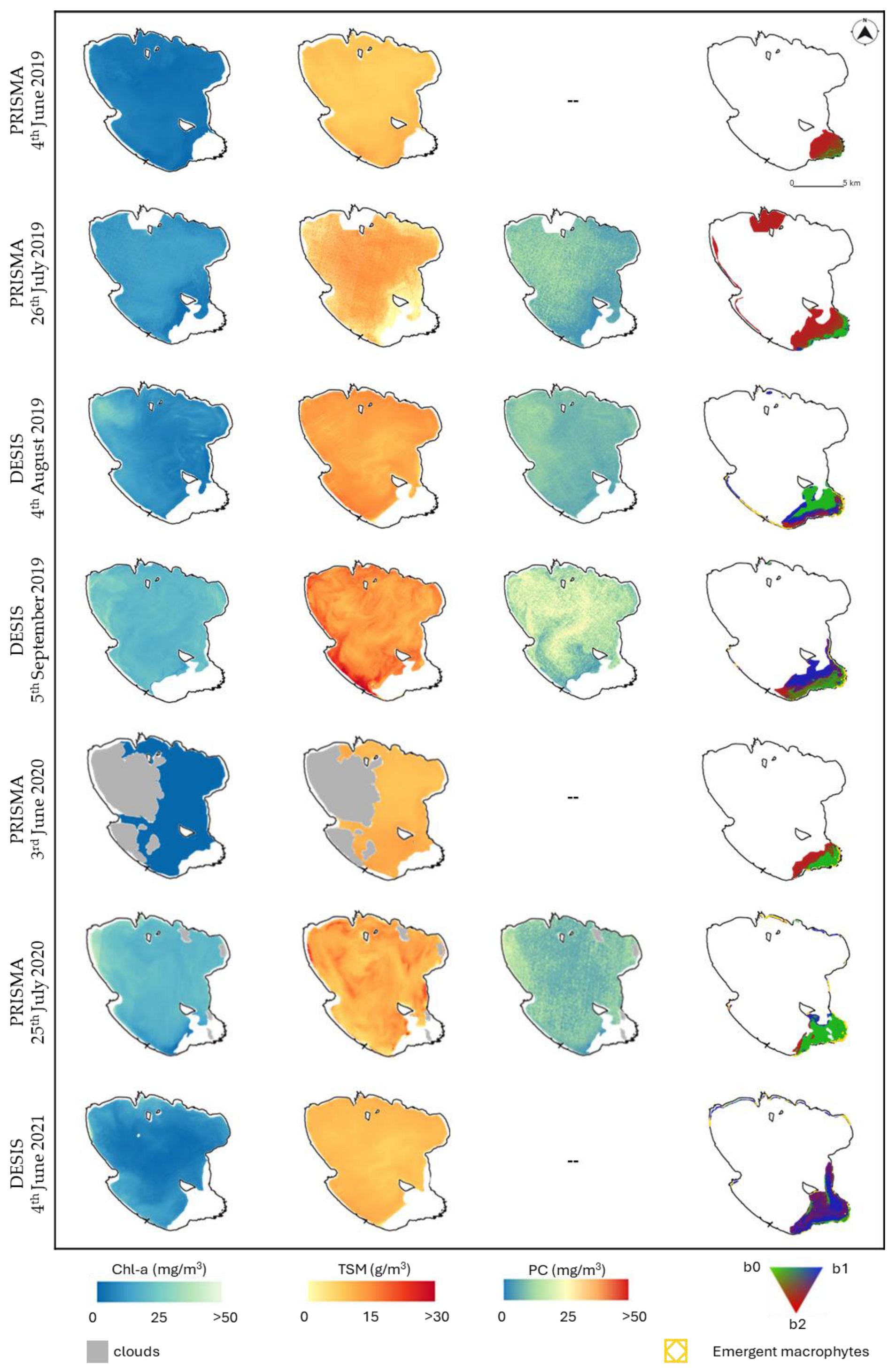
| Product | Submerged Macrophytes | Emergent Macrophytes |
|---|---|---|
| PRISMA 4 June 2019 | 135 ha (1.1%) | 0 ha |
| PRISMA 26 July 2019 | 287 ha (2.4%) | 0 ha |
| DESIS 4 August 2019 | 1140 ha (10.1%) | 52 ha (0.5%) |
| DESIS 5 September 2019 | 1190 ha (10.3%) | 25 ha (0.2%) |
| PRISMA 3 June 2020 | 300 ha (3.4%) | 19 ha (0.2%) |
| PRISMA 25 July 2020 | 878 ha (7.9%) | 37 ha (0.3%) |
| DESIS 4 June 2021 | 1523 ha (13.6%) | 33 ha (0.3%) |
| DESIS 15 October 2021 | 601 ha (5.1%) | 3 ha (<0.1%) |
| DESIS 19 June 2022 | 1790 ha (16.7%) | 149 ha (1.4%) |
| PRISMA 20 July 2022 | 2672 ha (23.0%) | 336 ha (2.9%) |
| DESIS 7 August 2022 | 1350 ha (12.3%) | 324 ha (3.0%) |
| PRISMA 12 August 2022 | 1223 ha (11.7%) | 343 ha (3.3%) |
| EnMAP 5 October 2022 | 344 ha (3.0%) | 199 ha (1.7%) |
Disclaimer/Publisher’s Note: The statements, opinions and data contained in all publications are solely those of the individual author(s) and contributor(s) and not of MDPI and/or the editor(s). MDPI and/or the editor(s) disclaim responsibility for any injury to people or property resulting from any ideas, methods, instructions or products referred to in the content. |
© 2024 by the authors. Licensee MDPI, Basel, Switzerland. This article is an open access article distributed under the terms and conditions of the Creative Commons Attribution (CC BY) license (https://creativecommons.org/licenses/by/4.0/).
Share and Cite
Fabbretto, A.; Bresciani, M.; Pellegrino, A.; Alikas, K.; Pinardi, M.; Mangano, S.; Padula, R.; Giardino, C. Tracking Water Quality and Macrophyte Changes in Lake Trasimeno (Italy) from Spaceborne Hyperspectral Imagery. Remote Sens. 2024, 16, 1704. https://doi.org/10.3390/rs16101704
Fabbretto A, Bresciani M, Pellegrino A, Alikas K, Pinardi M, Mangano S, Padula R, Giardino C. Tracking Water Quality and Macrophyte Changes in Lake Trasimeno (Italy) from Spaceborne Hyperspectral Imagery. Remote Sensing. 2024; 16(10):1704. https://doi.org/10.3390/rs16101704
Chicago/Turabian StyleFabbretto, Alice, Mariano Bresciani, Andrea Pellegrino, Krista Alikas, Monica Pinardi, Salvatore Mangano, Rosalba Padula, and Claudia Giardino. 2024. "Tracking Water Quality and Macrophyte Changes in Lake Trasimeno (Italy) from Spaceborne Hyperspectral Imagery" Remote Sensing 16, no. 10: 1704. https://doi.org/10.3390/rs16101704