
A Novel Iterative Thresholding Algorithm Based on Plug-and-Play Priors for Compressive Sampling


School of Electronic and Information Engineering, South China University of Technology, Guangzhou 510641, China
*
Author to whom correspondence should be addressed.
Future Internet 2017, 9(3), 24; https://doi.org/10.3390/fi9030024
Submission received: 17 May 2017
/
Revised: 19 June 2017
/
Accepted: 21 June 2017
/
Published: 24 June 2017
Abstract
:We propose a novel fast iterative thresholding algorithm for image compressive sampling (CS) recovery using three existing denoisers—i.e., TV (total variation), wavelet, and BM3D (block-matching and 3D filtering) denoisers. Through the use of the recently introduced plug-and-play prior approach, we turn these denoisers into CS solvers. Thus, our method can jointly utilize the global and nonlocal sparsity of images. The former is captured by TV and wavelet denoisers for maintaining the entire consistency; while the latter is characterized by the BM3D denoiser to preserve details by exploiting image self-similarity. This composite constraint problem is then solved with the fast composite splitting technique. Experimental results show that our algorithm outperforms several excellent CS techniques.
1. Introduction
In compressive sampling [1,2], we aim to estimate an image from m < n linear observations y , , where A is the measurement matrix. Since m < n, this problem is ill-posed. In order to solve this ill-posed problem, one needs some prior knowledge [3,4]. Therefore, researchers have explored the use of sophisticated structures to reflect the image priors, such as minimal total variation [5], wavelet trees [6,7], Markov mixture models [8], and non-local sparsity [9,10,11,12,13,14,15].
To establish these complicated models for image CS recovery, penalty functions are frequently used to encourage solutions of a certain form [5,6,11]. In FCSA (Fast Composite Splitting Algorithm) [5], sparsity penalty terms in wavelet and gradient domain are jointly used to constrain the solution space; while WaTMRI (wavelet tree sparsity magnetic resonance imaging) [6] superadds a tree sparse regularization to the objective function of FCSA, further forcing the parent-child wavelet coefficients to be zeros or non-zeros together. On the other hand, in Bayesian CS [8,12], graphical models are employed to describe the probabilistic relationship between measurements and the original signal. In [8], the structure of the wavelet coefficients is modeled by a hidden Markov tree (HMT).
Among these structures, nonlocal sparsity [11,12,15], which exploits the self-repetitive structure exhibited often in natural images has shown great potential. In NLR-CS (CS via nonlocal low-rank regularization) [11], a patch-based low-rank regularization model is built to enforce the low-rank property over the sets of nonlocal similar patches; while RCoS (CS recovery via collaborative sparsity) [14] uses a 3D sparsity term to maintain image nonlocal consistency. In contrast, the D-AMP (denoising-based approximate message passing) algorithm [12] exploits the image self-similarity through the use of nonlocal based denoisers, such as the BM3D (block-matching and 3D filtering) denoiser [16], which performs hard or soft thresholding with a 3D orthogonal dictionary (3D filtering) on 3D image blocks built by stacking similar patches together (block-matching). Closely relating to D-AMP, BM3D-CS [15] iteratively adds noise to the missing part of the spectra and then applies BM3D to the result. However, the above signal models cannot simultaneously utilize the global and nonlocal sparsity. Although the nonlocal sparse regularization can preserve image fine details by clustering similar components, it is based on block matching, and thus introduces visible artifacts in homogeneous regions, manifesting as low-frequency noise [17]. On the other hand, TV and wavelet sparse regularization can maintain the consistency of the entire image.
In this paper, we propose an iterative thresholding method that is competitive in quality with D-AMP, but is much simpler to implement. We combine three popular denoisers through the use of the plug-and-play prior approach [18,19], which is able to turn a denoiser into reconstruction solver. For charactering the nonlocal sparsity, we use the nonlocal wavelet denoiser. For representing the global sparsity, we use the wavelet and gradient denoiser. This multiple denoisers problem is then solved based on fast composite splitting technique [5] and the fast proximal method FISTA (fast iterative shrinkage-thresholding algorithm) [20,21]. In the frame of FISTA, the original composite regularization problem is firstly decomposed into three simpler regularization sub-problems via fast composite splitting technique; then each of them is separately solved by thresholding methods. Experimental results show that our method impressively outperforms previous methods in terms of reconstruction accuracy, and also achieves competitive advantage in computation complexity.
2. Compressive Sampling and Fast Iterative Shrinkage-Thresholding Algorithm
The compressive sampling recovery is an underdetermined problem. More than one solution can yield the same measurements, but if x is sparse, we can recover the original signal by minimizing the following L1 problem.
where is a regularization parameter.
The above problem can be efficiently solved by various methods [22,23,24,25], one of which is ISTA (iterative shrinkage-thresholding algorithm) [26]. Specifically, the general step of ISTA is summarized in Algorithm 1, where , and denotes the gradient of the function f at the point ; denotes the conjugate transpose of A; c is a step size. The undersampled Fourier matrix A = SF is used as the measurement matrix, where F is the 2D Fourier transform and S is a selection matrix containing m rows of the identity matrix. Step (b) is a proximity operator. It has a close form solution, which can be expressed as:
FISTA [21] offers an accelerated version of ISTA by adding an accelerated step (step (c)), which is summarized in Algorithm 2.
| Algorithm 1. ISTA [26] |
| Input: the CS measurements y and the measurement matrix A |
| Initialization: x0 = 0, |
| for k = 1 to K do |
| (a) |
| (b) |
| end for |
| Algorithm 2. FISTA [21] |
| Input: the CS measurements y and the measurement matrix A |
| Initialization: x0 = r1 = 0, |
| for k = 1 to K do |
| (a) |
| (b) |
| (c) ; |
| end for |
3. CS via Composite Regularization and Adaptive Thresholding
3.1. The New Composite Model
Images are generally sparse in wavelet and gradient domain, although not strictly. Moreover, there exist abundant similar image patches in natural images. These sparse priors can be utilized by using three regularizations (TV, wavelet sparse, and nonlocal wavelet regularization). The nonlocal sparse regularization can preserve image fine details, while TV and wavelet sparse regularization can maintain the consistency of the entire image. In order to gain the advantages of these regularizations, we combine the nonlocal self-similarity of patches and the global sparsity in wavelet and gradient domain to jointly enforce the solution in image CS recovery, and formulate a composite regularization problem as:
where , , and are three regularization parameters. The first item is the fidelity term; while the last three items are priori constraint terms, denoting TV norm, wavelet sparse norm, and nonlocal wavelet norm respectively. Usually, the TV norm of a 2D image X with size p × q is computed by:
and the wavelet sparse norm can be represented as where is the wavelet transform. However, these regularizations are equal to denoising operations in the solving process by adopting the plug-and-play prior approach. We characterize the image self-similarity by means of the last item in Equation (3) derived from BM3D [15], which is used to seek patch correlation in image denoising. To construct , we first stack similar image patches to 3D groups, then 3D wavelet transform is conduct on each 3D group, which is achieved by conducting 2D wavelet transform on each patch and then conducting 1D wavelet transform along the third axis.
3.2. Solving The Composite Model with Fast Composite Splitting Technique
We solve the above composite regularization problem Equation (3) based on FISTA algorithm and fast composite splitting technique [5] which decomposes the original composite problem into simpler regularization sub-problems, separately solves each of them, and then obtains the final solution by a linear combination. Algorithm 3 outlines the solving procedure of our algorithm named as PPP-CS (CS with plug-and-play priors). In step (a), the fidelity term is computed with gradient descent method to get an initial solution xg. In steps (b)–(d), variable x is split into three variables x1, x2 and x3; the corresponding proximity operator is performed over each of them. In step (e) the solution xk is obtained by linear combination of x1, x2, and x3. Step (f) is the acceleration step borrowed from FISTA. The convergence of PPP-CS is guaranteed by fast composite splitting technique and FISTA algorithm.
| Algorithm 3. CS with Plug-and-play Priors |
| Input: the CS measurements y and the measurement matrix A |
| Initialization: x0 = r1 = 0, , , c |
| for k = 1 to K do |
| (a) |
| (b) |
| (c) |
| (d) |
| (e) |
| (f) ; |
| end for |
Steps (b)–(d) are the so-called proximal map, which is formally defined in [27], i.e., given a continuous convex function and any scalar , the proximal map associated to function g is defined as:
In the plug-and-play prior approach [18,19], this proximal map is equal to a denoising operation, where is a noisy image, is a regularization corresponding to a denoiser, and is the denoising threshold. In the steps (b)–(d), we regard xg as a noisy image; then the corresponding denoising methods can be adopted to obtain the solution of each sub-problem. For step (b), we use a TV-based denoising method which is based on the FISTA algorithm [27]. For step (c), the wavelet denoisers are available; but we can solve this sub-problem easily, since it has a close form solution, which can be computed with soft thresholding (see Equation (2)). For step (d), we use the BM3D denoiser [15].
The key to success in solving Equation (3) is to determine the denoising threshold of the BM3D denoiser. The original threshold of BM3D is proportional to the noise variance of image; however, it is hard to estimate the noise variance of the current image in the CS reconstruction. Apparently, the denoising threshold should be reduced along with the iteration as the recovered image becomes more and more clear. Therefore, a natural idea is that it should be proportional to the observation residual in CS reconstruction.
where s is a scale factor and can be set empirically.
4. Experiments
To evaluate reconstruction performances of the proposed algorithm in items of average PSNR (peak signal to noise ratio), runtime, and visual quality, we compare our algorithm with four excellent algorithms. There are two algorithms based on iterative shrinkage-thresholding method FCSA [1] (using wavelet sparsity and gradient sparsity), WaTMRI [2] (using wavelet sparsity, gradient sparsity and tree sparsity) and two Bayesian CS methods Turbo-AMP [3] (using tree sparsity), D-AMP [6] (using nonlocal sparsity via BM3D denoiser). Three experiments are carried on both natural images and MR (Magnetic Resonance) images with size 256 × 256 at four sampling ratios (18, 20, 22, and 25%). The eight natural images and four MR images used in our experiments are shown in Figure 1. The undersampled Fourier matrix is generated by following the previous works [2,3], which randomly choose more Fourier coefficients from low frequency and less on high frequency. All experiments are on a desktop with 3.80 GHz AMD A10-5800K CPU. Matlab version is 7.11 (R2010b).
We set the maximum iterations K = 10 for Turbo-AMP and set K = 50 for the rest algorithms. For our algorithm PPP-CS, we use the setting = 0.001, = 0.023, c = 1. The scale factor in Equation (6) s is set to 30 in the first 20 iterations, and is fixed at 5 after 20 iterations; since the estimated threshold is basically steady at that moment. The 3D wavelet transform Г3D is composed of 2-D bior1.5 and 1-D Haar. To construct 3D groups by stacking similar patches, we need to set the following parameters: the size of each patch is 8 × 8 pixels the size of window for searching matched patches is 25 × 25 pixels; the number of best matched patches is 16; and the sliding step to process every next reference patch is set to 6. After the first five iterations, step (d) is only updated every three iterations in order to speed up the algorithm. For the rest algorithms, the default settings in their codes are used.
4.1. Quantative Evaluation
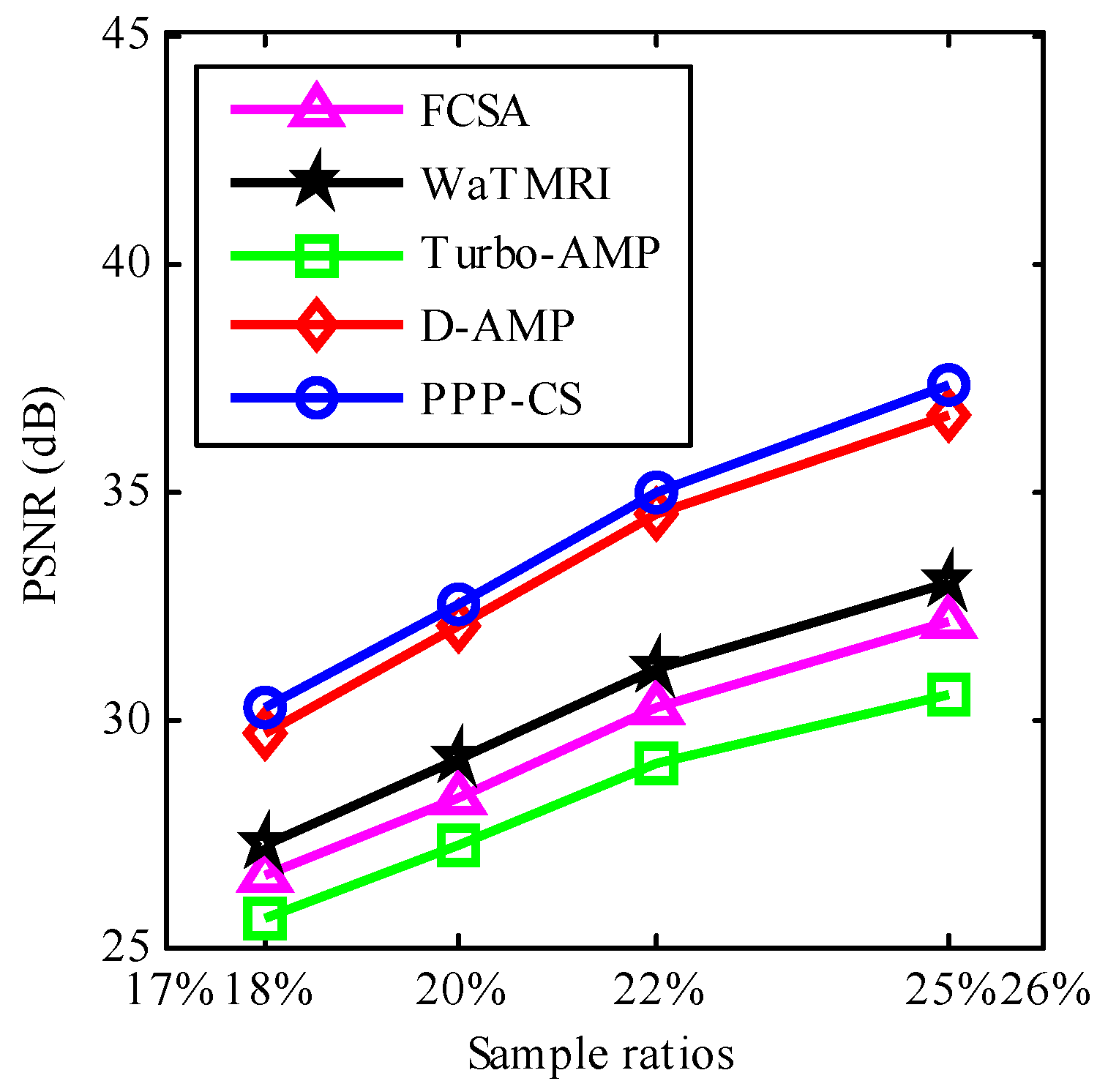
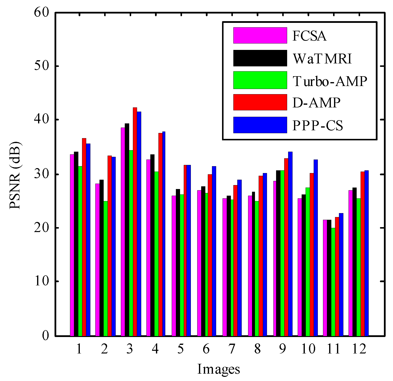
We carry all algorithms on the 12 test images with various sampling ratios, the average PSNR results by running each image five times are shown in Figure 2, from which we can see that the nonlocal sparsity-based methods PPP-CS and D-AMP are better than others. Particularly, the proposed algorithm PPP-CS achieves the highest PSNR results. By jointly using of the global and nonlocal sparsity, the proposed PPP-CS method performs much better than the D-AMP method on all sensing rates. The PSNR results of reconstructed images from the CS measurements with 20% sampling are included in Figure 3. One can see that the proposed PPP-CS method produces the highest PSNRs on almost all test images (except for three cases where PPP-CS slightly falls behind D-AMP). The average PSNR improvement over D-AMP is about 10.54 dB, which validates the superiority of the proposed algorithm in objective quality.
Figure 4 gives the average CPU time of different algorithms carried on the 12 test images by running each 5 times. FCSA spends the least CPU time; however, its PSNR results in Figure 1 are relatively poor. Note that PPP-CS spends 62.05% less CPU time to achieve higher PSNR than D-AMP, for the result that the Bayesian algorithm AMP is slower than our fast iterative shrinkage-thresholding algorithm.
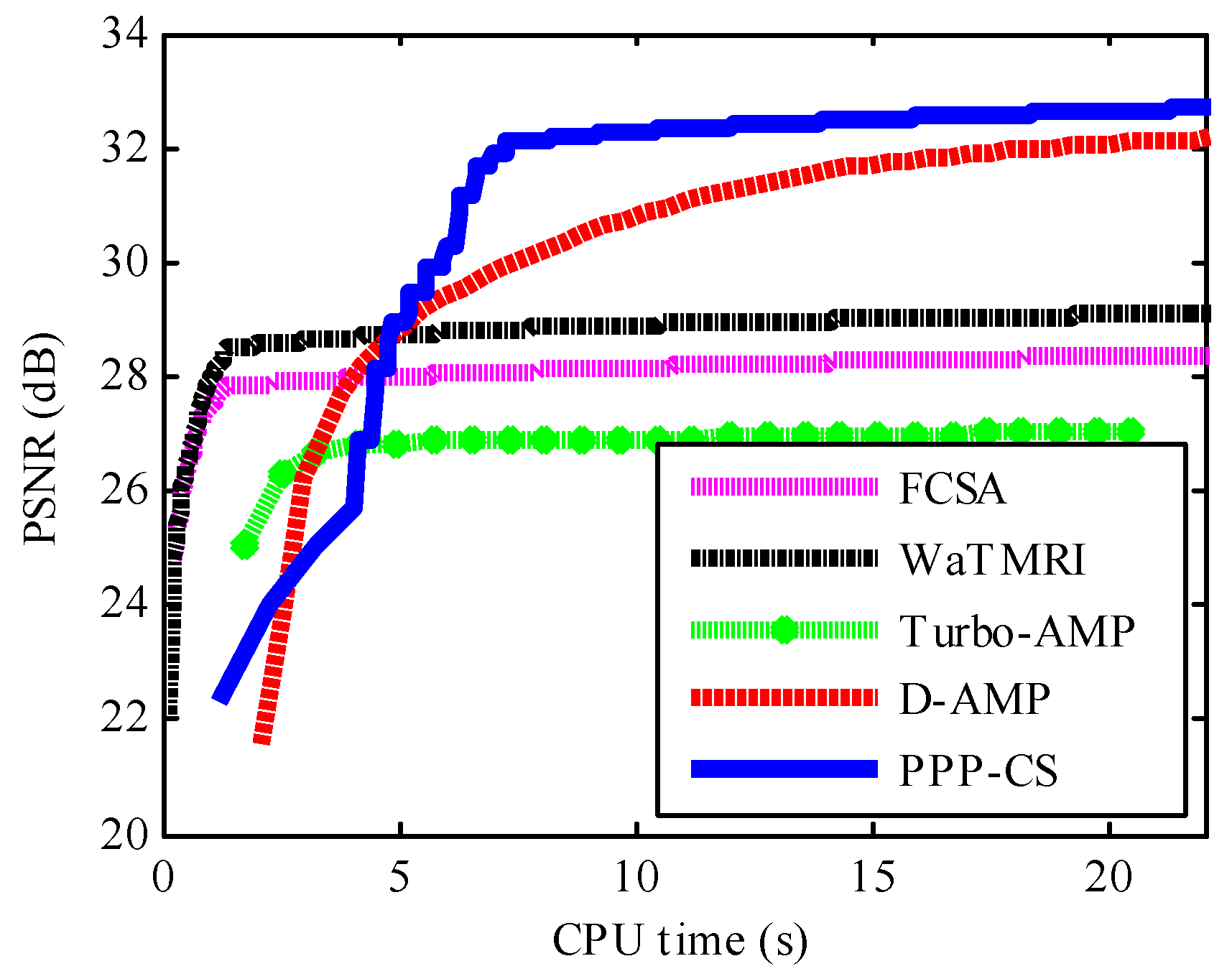
Figure 5 gives the performance comparisons between different methods in terms of the CPU time over the PSNR with 20% sampling. The PPP-CS obtains the best reconstruction results by achieving the highest PSNR in less CPU time after five seconds. Since PPP-CS is based on FISTA, it can converge fast. The D-AMP is inferior to the PPP-CS for most of the time, because of its higher cost in each iteration. These results show the effectiveness of acceleration strategies in the PPP-CS inherited from the FISTA for the image reconstruction.
4.2. Visual Quality Evaluation
Figure 6 provides the CS recovery results for image Cameraman in the case of sample rate = 20% using the test algorithms. For each algorithm, we compute the PSNR as well as the structural similarity index (SSIM) which better reflects the visual quality of the images. From Figure 6, it is clear to see that the nonlocal sparsity-based methods PPP-CS and D-AMP are still better than others. The proposed algorithm enjoys great advantages over other competing algorithms in producing more clean screens, e.g., on the area of sky. Due to the joint use of the global and nonlocal sparsity and adaptive thresholding strategy, the elimination of artifacts is more effective by applying PPP-CS.
5. Conclusions
A new image compressive sampling recovery algorithm based on the FISTA algorithm and plug-and-play priors is proposed in this paper. Our contributions are as follows: (1) jointly using of the global and nonlocal sparsity to maintain entire consistency and preserve details in image CS recovery, which can be achieved through the use of the plug-and-play prior approach; (2) applying the FISTA algorithm and fast composite splitting technique to turn the complicated composite constraint problem into three independent shrinkage-thresholding problems, and obtain a simple implementation and a fast convergence rate. Finally, we combine the FISTA algorithm with plug-and-play priors for the first time, making it easy to use the powerful denoisers in CS reconstruction. In the experiments, our algorithm is shown to outperform four excellent algorithms in reconstructed quality, and also achieve competitive advantage in runtime.
Acknowledgments
This work is partially supported by the National Natural Science Foundation of China (No. 61302120), the Science and Technology Planning Project of Guangdong Province (No. 2017A020214011), the Fundamental Research Funds for the Central Universities (No. 2017MS039), and the Specialized Research Fund for the Doctoral Program of Higher Education (No. 20130172120045). The authors also gratefully acknowledge the helpful comments and suggestions of the reviewers, which have improved the presentation.
Author Contributions
Lingjun Liu and Zhonghua Xie conceived and designed the experiments; Zhonghua Xie performed the experiments; Lingjun Liu and Cui Yang analyzed the data; Lingjun Liu wrote the paper. All authors have read and approved the final manuscript.
Conflicts of Interest
The authors declare no conflict of interest.
References
- Donoho, D.L. Compressed sensing. IEEE Trans. Inf. Theory 2006, 52, 1289–1306. [Google Scholar] [CrossRef]
- Candès, E.J.; Romberg, J.; Tao, T. Robust uncertainty principles: Exact signal reconstruction from highly incomplete frequency information. IEEE Trans. Inf. Theory 2006, 52, 489–509. [Google Scholar] [CrossRef]
- Tan, J.; Ma, Y.; Baron, D. Compressive Imaging via Approximate Message Passing with Image Denoising. IEEE Trans. Signal Process. 2015, 63, 424–428. [Google Scholar] [CrossRef]
- Zhu, Z.; Qi, G.; Chai, Y.; Chen, Y. A Novel Multi-Focus Image Fusion Method Based on Stochastic Coordinate Coding and Local Density Peaks Clustering. Future Internet 2016, 8, 53–70. [Google Scholar] [CrossRef]
- Huang, J.; Zhang, S.; Metaxas, D. Efficient MR Image Reconstruction for Compressed MR Imaging. Med. Image Anal. 2011, 15, 670–679. [Google Scholar] [CrossRef] [PubMed]
- Chen, C.; Huang, J. Exploiting the wavelet structure in compressed sensing MRI. Magn. Reson. Imaging 2014, 32, 1377–1389. [Google Scholar] [CrossRef] [PubMed]
- Wang, M.; Wu, X.; Jing, W.; He, X. Reconstruction algorithm using exact tree projection for tree-structured compressive sensing. IET Signal Process. 2016, 10, 566–573. [Google Scholar] [CrossRef]
- Som, S.; Schniter, P. Compressive imaging using approxi- mate message passing and a markov-tree prior. IEEE Trans. Signal Process. 2012, 60, 3439–3448. [Google Scholar] [CrossRef]
- Zhang, X.; Bai, T.; Meng, H.; Chen, J. Compressive Sensing-Based ISAR Imaging via the Combination of the Sparsity and Nonlocal Total Variation. IEEE Geosci. Remote Sens. Lett. 2014, 11, 990–994. [Google Scholar] [CrossRef]
- Dong, W.; Shi, G.; Wu, X.; Zhang, L. A learning-based method for compressive image recovery. J. Vis. Commun. Image Represent. 2013, 24, 1055–1063. [Google Scholar] [CrossRef]
- Dong, W.; Shi, G.; Li, X.; Ma, Y.; Huang, F. Compressive sensing via nonlocal low-rank regularization. IEEE Trans. Image Process. 2014, 23, 3618–3632. [Google Scholar] [CrossRef] [PubMed]
- Metzler, C.A.; Maleki, A.; Baraniuk, R.G. From Denoising to Compressed Sensing. IEEE Trans. Inf. Theory 2016, 62, 5117–5144. [Google Scholar] [CrossRef]
- Metzler, C.A.; Maleki, A.; Baraniuk, R.G. BM3D-AMP: A New Image Recovery Algorithm Based on BM3D Denoising. In Proceedings of the IEEE International Conference on Image Processing (ICIP), Quebec City, QC, Canada, 27–30 September 2015; pp. 3116–3120. [Google Scholar]
- Zhang, J.; Zhao, D.; Zhao, C.; Xiong, R.; Ma, S.; Gao, W. Image Compressive Sensing Recovery via Collaborative Sparsity. IEEE J. Emerg. Sel. Top. Circuits Syst. 2012, 2, 380–391. [Google Scholar] [CrossRef]
- Egiazarian, K.; Foi, A.; Katkovnik, V. Compressed Sensing Image Reconstruction via Recursive Spatially Adaptive Filtering. In Proceedings of the IEEE International Conference on Image Processing (ICIP), San Antonio, TX, USA, 16–19 September 2007; pp. I-549–I-552. [Google Scholar]
- Dabov, K.; Foi, A.; Katkovnik, V.; Egiazarian, K. Image denoising by sparse 3-D transform-domain collaborative filtering. IEEE Trans. Image Process. 2007, 16, 2080–2095. [Google Scholar] [CrossRef] [PubMed]
- Knaus, C.; Zwicker, M. Dual-Domain Filtering. SIAM J. Imaging Sci. 2015, 8, 1396–1420. [Google Scholar] [CrossRef]
- Venkatakrishnan, S.; Bouman, C.A.; Wohlberg, B. Plug-and-Play Priors for Model Based Reconstruction. In Proceedings of the IEEE Global Conference on Signal and Information Processing (Global SIP), Austin, TX, USA, 3–5 December 2013; pp. 945–948. [Google Scholar]
- Brifman, A.; Romano, Y.; Elad, M. Turning a Denoiser into a Super-Resolver Using Plug and Play Priors. In Proceedings of the IEEE International Conference on Image Processing (ICIP), Phoenix, AZ, USA, 25–28 September 2016; pp. 1404–1408. [Google Scholar]
- Liu, L.; Xie, Z.; Feng, J. Backtracking-Based Iterative Regularization Method for Image Compressive Sensing Recovery. Algorithms 2017, 10, 1–8. [Google Scholar] [CrossRef]
- Beck, A.; Teboulle, M. A fast iterative shrinkage-thresholding algorithm for linear inverse problems. SIAM J. Imaging Sci. 2009, 2, 183–202. [Google Scholar] [CrossRef]
- Hosseini, M.S.; Plataniotis, K.N. High-accuracy total variation with application to compressed video sensing. IEEE Trans. Image Process. 2014, 23, 3869–3884. [Google Scholar] [CrossRef] [PubMed]
- Ling, Q.; Shi, W.; Wu, G.; Ribeiro, A. DLM: Decentralized Linearized Alternating Direction Method of Multipliers. IEEE Trans. Signal Process. 2015, 63, 4051–4064. [Google Scholar] [CrossRef]
- Yin, W.; Osher, S.; Goldfarb, D.; Darbon, J. Bregman iterative algorithms for l1-minimization with applications to compressed sensing. SIAM J. Imaging Sci. 2008, 1, 143–168. [Google Scholar] [CrossRef]
- Qiao, T.; Li, W.; Wu, B. A New Algorithm Based on Linearized Bregman Iteration with Generalized Inverse for Compressed Sensing. Circuits Syst. Signal Process. 2014, 33, 1527–1539. [Google Scholar] [CrossRef]
- Daubechies, I.; Defriese, M.; DeMol, C. An iterative thresholding algorithm for linear inverse problems with a sparsity constraint. Commun. Pure Appl. Math. 2004, 57, 1413–1457. [Google Scholar] [CrossRef]
- Beck, A.; Teboulle, M. Fast gradient-based algorithms for constrained total variation image denoising and deblurring problems. IEEE Trans. Image Process. 2009, 18, 2419–2434. [Google Scholar] [CrossRef] [PubMed]
Figure 1.
Twelve experimental test images.
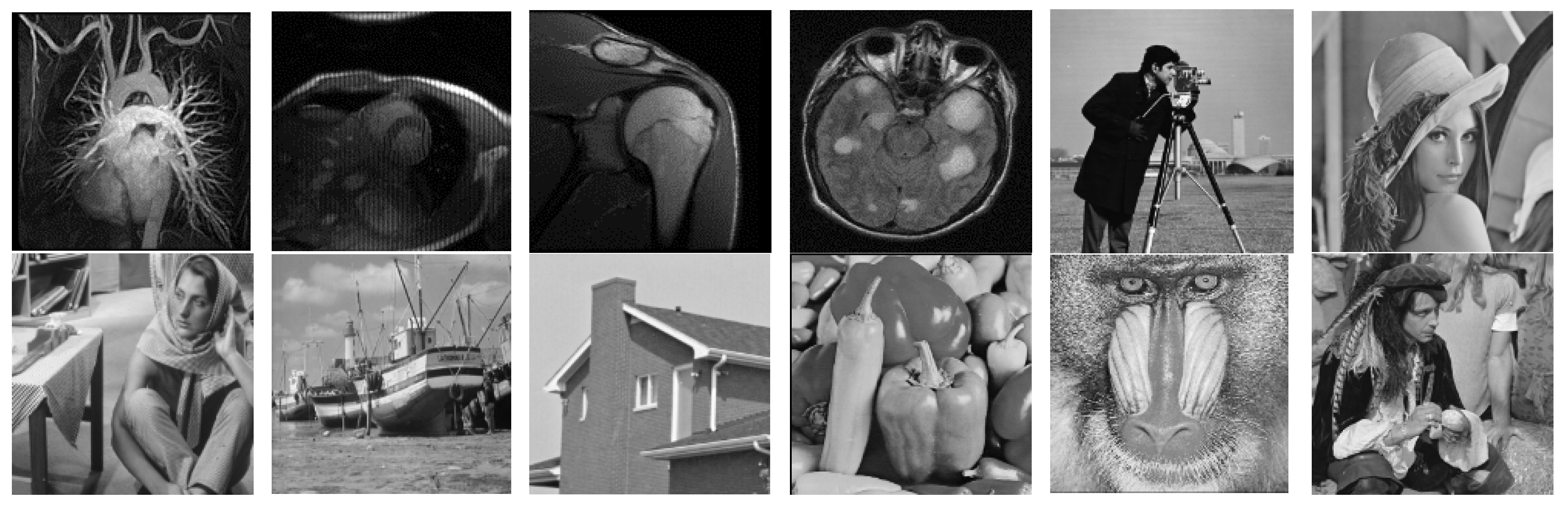
Figure 2.
Average PSNR (peak signal to noise ratio) (dB) comparisons on the 12 test images with various sampling ratios.
Figure 2.
Average PSNR (peak signal to noise ratio) (dB) comparisons on the 12 test images with various sampling ratios.

Figure 3.
Average PSNR (dB) of different images with 20% sampling.

Figure 4.
Average CPU time (s) comparisons on the 12 test images with various sampling ratios.
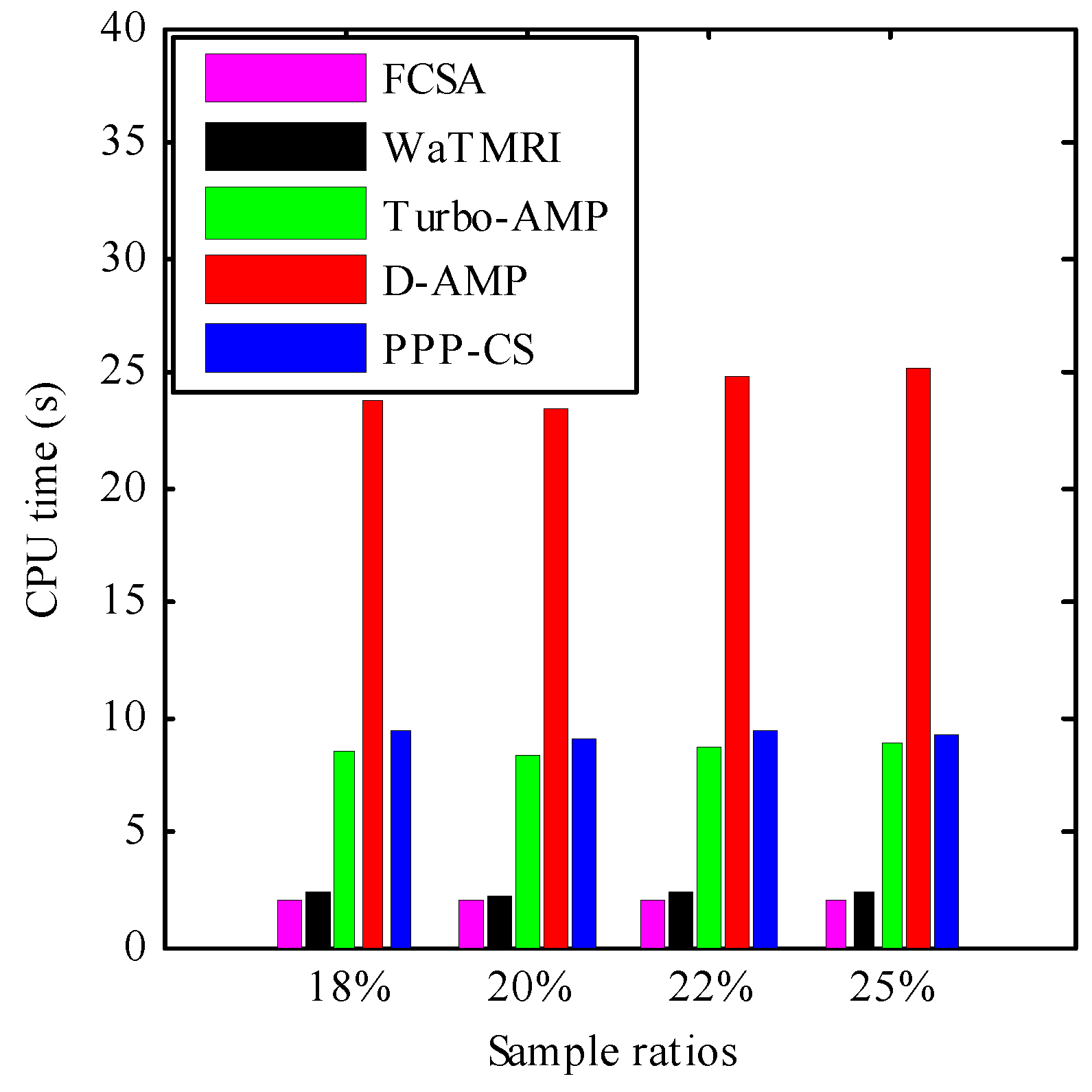
Figure 5.
Performance comparison (CPU time vs. PSNR) with 20% sampling.

Figure 6.
Visual quality comparison of image CS recovery using different algorithms for image “Cameraman” in the case of sample rate = 20%. (a) The original; (b) FCSA (PSNR = 25.92 dB, SSIM = 0.6784); (c) WaTMRI (PSNR = 27.07 dB, SSIM = 0.7451); (d) Turbo-AMP (PSNR = 27.48 dB, SSIM = 0.8523); (e) D-AMP (PSNR = 31.01 dB, SSIM = 0.9329); (f) PPP-CS (PSNR = 32.73 dB, SSIM = 0.9448).
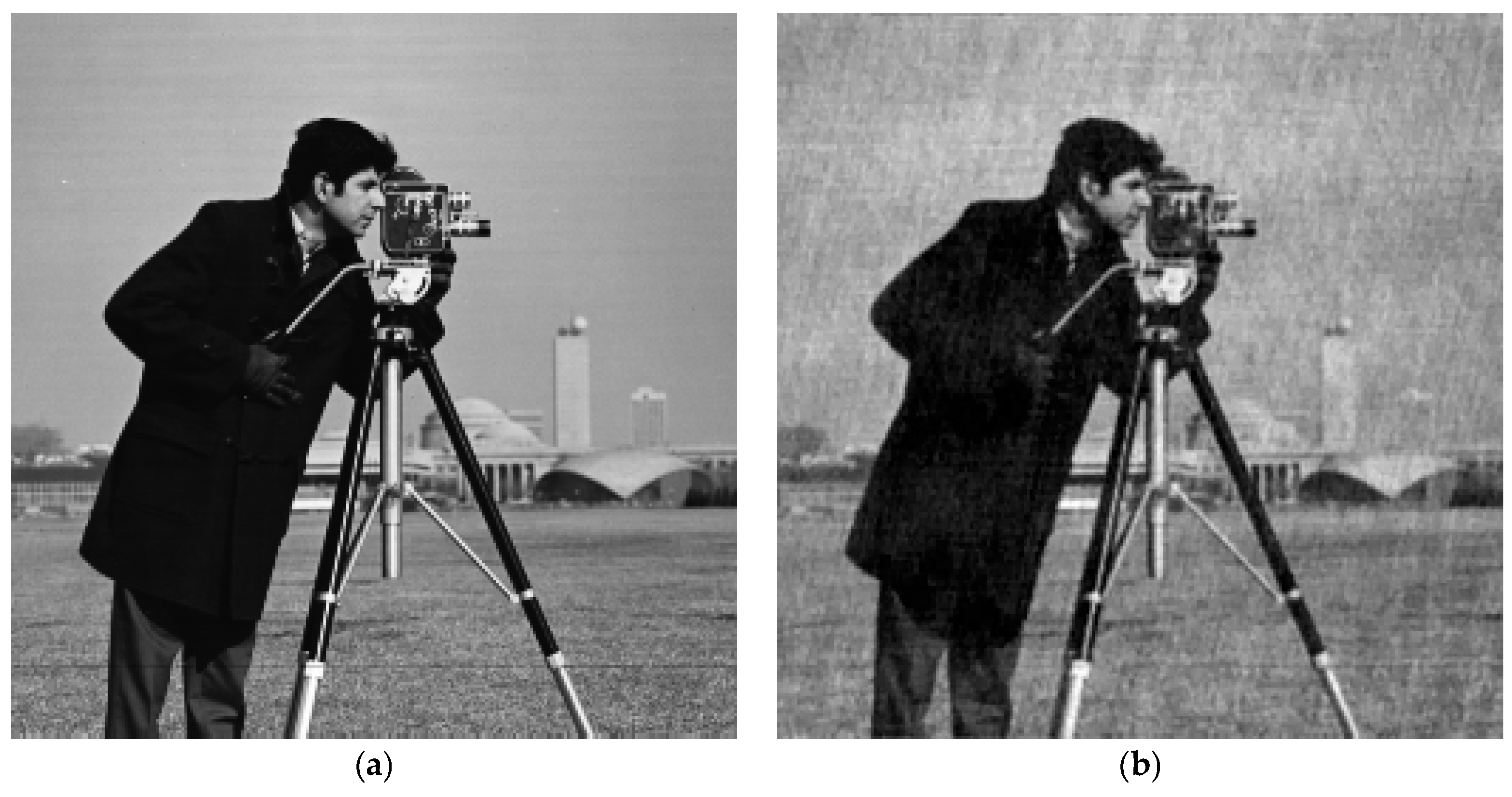
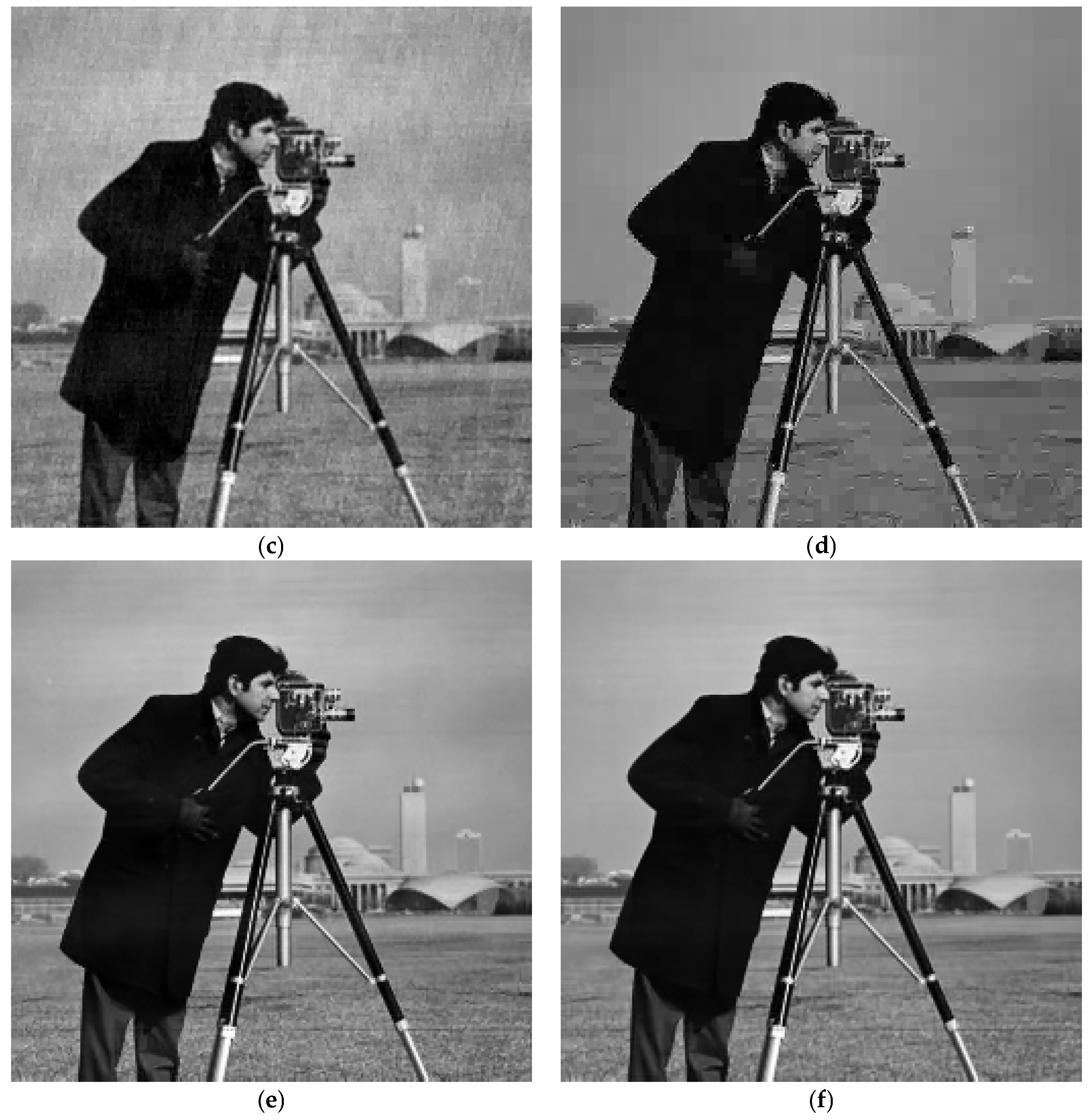
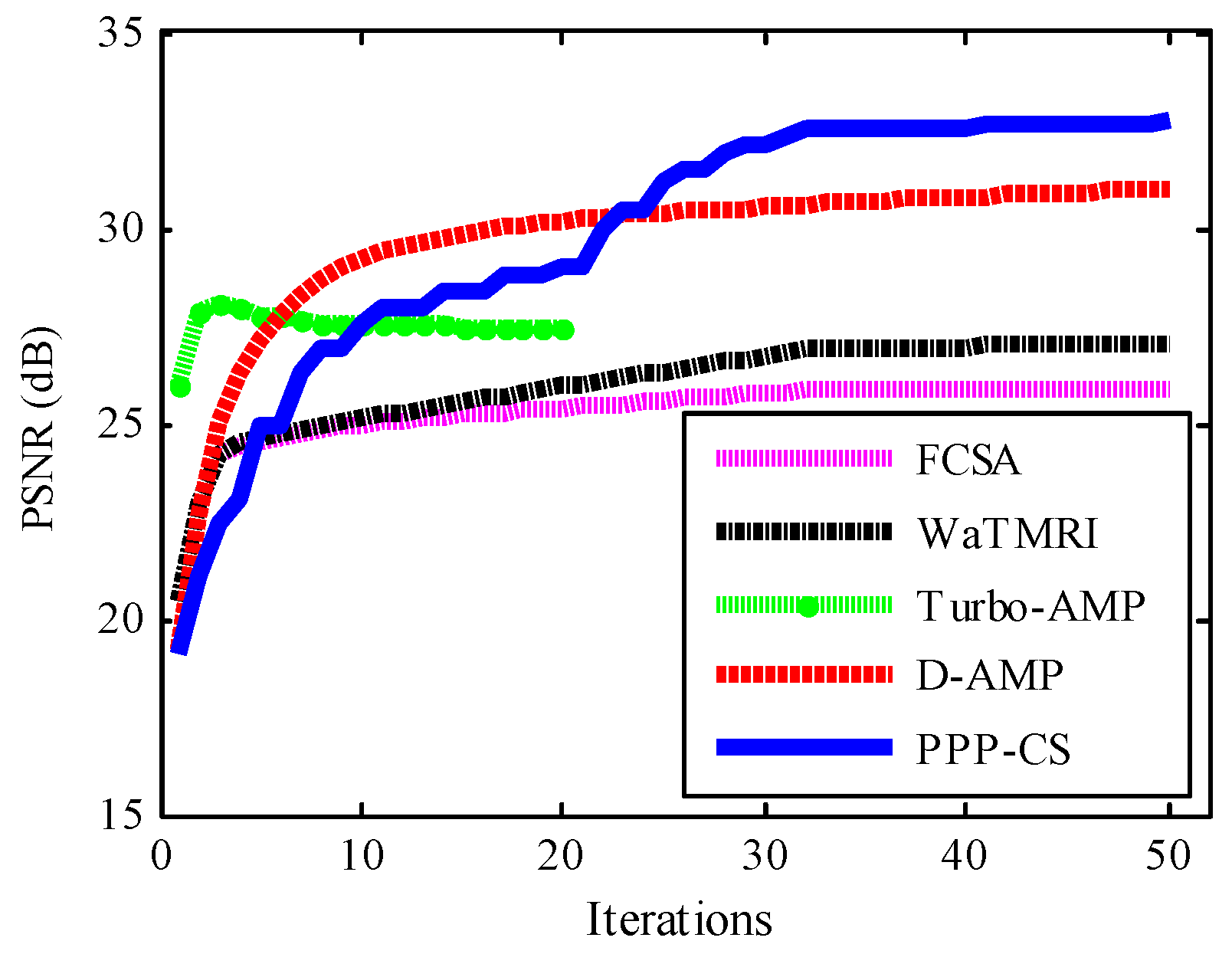
Figure 7.
Performance comparison (iterations vs. PSNR) on “Cameraman” with 20% sampling.

Figure 8.
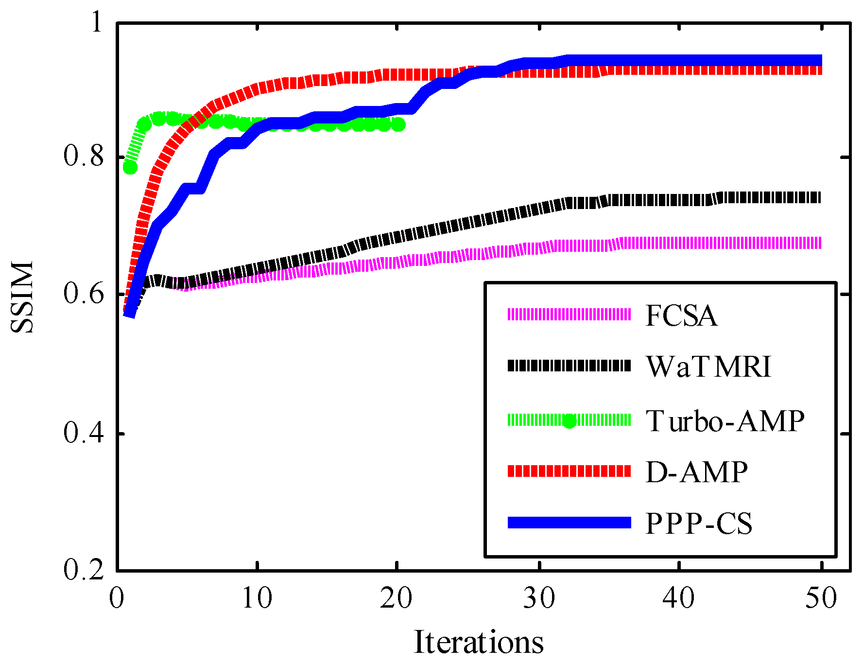
Performance comparison (iterations vs. SSIM) on “Cameraman” with 20% sampling.

© 2017 by the authors. Licensee MDPI, Basel, Switzerland. This article is an open access article distributed under the terms and conditions of the Creative Commons Attribution (CC BY) license (http://creativecommons.org/licenses/by/4.0/).
Share and Cite
MDPI and ACS Style
Liu, L.; Xie, Z.; Yang, C. A Novel Iterative Thresholding Algorithm Based on Plug-and-Play Priors for Compressive Sampling. Future Internet 2017, 9, 24. https://doi.org/10.3390/fi9030024
AMA Style
Liu L, Xie Z, Yang C. A Novel Iterative Thresholding Algorithm Based on Plug-and-Play Priors for Compressive Sampling. Future Internet. 2017; 9(3):24. https://doi.org/10.3390/fi9030024
Chicago/Turabian StyleLiu, Lingjun, Zhonghua Xie, and Cui Yang. 2017. "A Novel Iterative Thresholding Algorithm Based on Plug-and-Play Priors for Compressive Sampling" Future Internet 9, no. 3: 24. https://doi.org/10.3390/fi9030024
Note that from the first issue of 2016, this journal uses article numbers instead of page numbers. See further details here.