Adaptive Holography in Liquid Crystal Light-Valves

1
INLN, Université de Nice-Sophia Antipolis, CNRS,1361 route des Lucioles, 06560 Valbonne, France
2
Jphopto, 20 Rue Campo Formio, 75013 Paris, France
*
Author to whom correspondence should be addressed.
Materials 2012, 5(9), 1546-1559; https://doi.org/10.3390/ma5091546
Submission received: 18 July 2012
/
Revised: 13 August 2012
/
Accepted: 20 August 2012
/
Published: 27 August 2012
(This article belongs to the Special Issue Advanced Materials for Modern Holographic Applications)
Abstract
:By performing two-wave mixing experiments in a liquid crystal light-valve, optical beam amplification is obtained as a strongly resonant process to which a narrow frequency bandwidth is associated. This property is exploited to realize adaptive holographic interferometric systems able to efficiently detect displacements as small as fraction of picometers. Pressure radiation induced deformations of a reflecting membrane are measured with the same type of system. Then, when used with complex wavefronts, like speckle fields, the LCLV-based interferometer allows to detect extremely small phase modulations. The examples shown demonstrate the potentialities of the light-valve for dynamic holography applications.
1. Introduction
Since its early developments in photorefractive crystals, dynamic holography has demonstrated great potentialities for applications in different fields such as image storage and processing [1], vibration analysis [2] and continuous reconstruction of interferograms [3]. After the seminal paper of Petrov on adaptive holographic interferometry (AHI) [4], the possibility of using the dynamic holographic recording technique to achieve highly precise measurements of small displacements has been demonstrated in numerous systems [5]. Since then, AHI has been proved as a useful tool for measuring small vibration amplitudes of reflecting objects [6,7,8,9]. A similar technique has been recently employed to realize acousto-optic imaging [10]. As a general rule, the physical mechanisms at the basis of the AHI rely on resonant two-wave mixing processes, whose associated narrow frequency bandwidth realizes the filtering function allowing to reject low frequency noise and environmental disturbances.
Starting from the last 30 years a lot of research has been devoted to photorefractive materials and their applications [11], while in the last decade spatial light modulators (SLM) have also attracted a great deal of attention and have emerged as important components for optical processing [12]. Indeed, SLMs are able to affect the phase modulation and the intensity of a readout beam, thus permitting the manipulation of information in the optical domain. In optically addressed SLM the control signal is provided by an optical input beam, so that optical parallelism can be fully exploited [13]. The general structure of an optically addressed SLM comprises two components: the photoreceptor and the electro-optic material, often separated by a dielectric mirror [14]. The input beam activates the photoreceptor which produces a corresponding charge field on the electro-optic material. The read light is modulated in its double pass through the electro-optic element in a retroreflective scheme. Since the readout can provide optical gain, this type of optically addressed SLM has also been called a light-valve. Historically, the photoreceptor has been a photoconductor, such as selenium or cadmium sulfide [15], amorphous silicon [16] or GaAs [17], and the electro-optic material has been a nematic liquid crystal layer, either in the parallel or twisted configuration [18], so that optically addressable SLM are also more widely known as liquid-crystal light-valves, LCLV.
An interesting type of LCLV has been realized by associating nematic liquid crystals with photorefractive crystals. The first photorefractive LCLV has been prepared by using as a photoconductor a thin monocrystalline (BSO) crystal [19]. The BSO, well known for its photorefractive properties, is chosen for its large photoconductivity and dark resistance, while its transparency in the visible range allows the LCLV working in transmissive configurations, where the input and readout beams may in general coincide. These features make of the photorefractive LCLVs optical elements with attractive capabilities for numerous applications, as laser beam manipulation [20], coherent image amplification through dynamic holography [21], transverse pattern formation [22], optical beam amplification [23], wave-mixing [24], slow-light [25,26,27] and manipulation of singular beams [28]. Here, we will focus on two-beam coupling experiments and to the creation of dynamical holograms. By this way, adaptive holographic interferometry can be performed with the LCLV, in close analogy to what previously described with photorefractive crystals. The main advantage of the LCLV is that photoconductive and electro-optic properties are separately optimized, so that an excellent photosensitivity comes from the large photoconductivity of the BSO and a large nonlinear response comes from the high birefringence of the nematic liquid crystals. This is particularly important in view of the adaptive holography applications, since it allows decreasing considerably the required laser power. Moreover, the possibility to obtain large (lateral size of a few centimeters) BSO crystals with a high degree of spatial homogeneity and uniform dark resistance makes LCLV very attractive for operating over large areas, hence allowing interferometry with spatially extended optical beams.
The paper is organized as follows. In Section 2 we present the LCLV and its main characteristics. In Section 3 the basics of the two-wave mixing in the LCLV are reviewed. In Section 4 we present the theoretical background of adaptive holography in the LCLV and we derive the theoretical limit of the minimum detectable displacement. In Section 5 we report some representative experimental results, showing the ability to detect sub-picometer displacements of vibrating objects as well the possibility to reveal extremely small phase modulations in complex wavefronts. Finally, Section 6 are the conclusions.
2. The Liquid Crystal Light-Valve
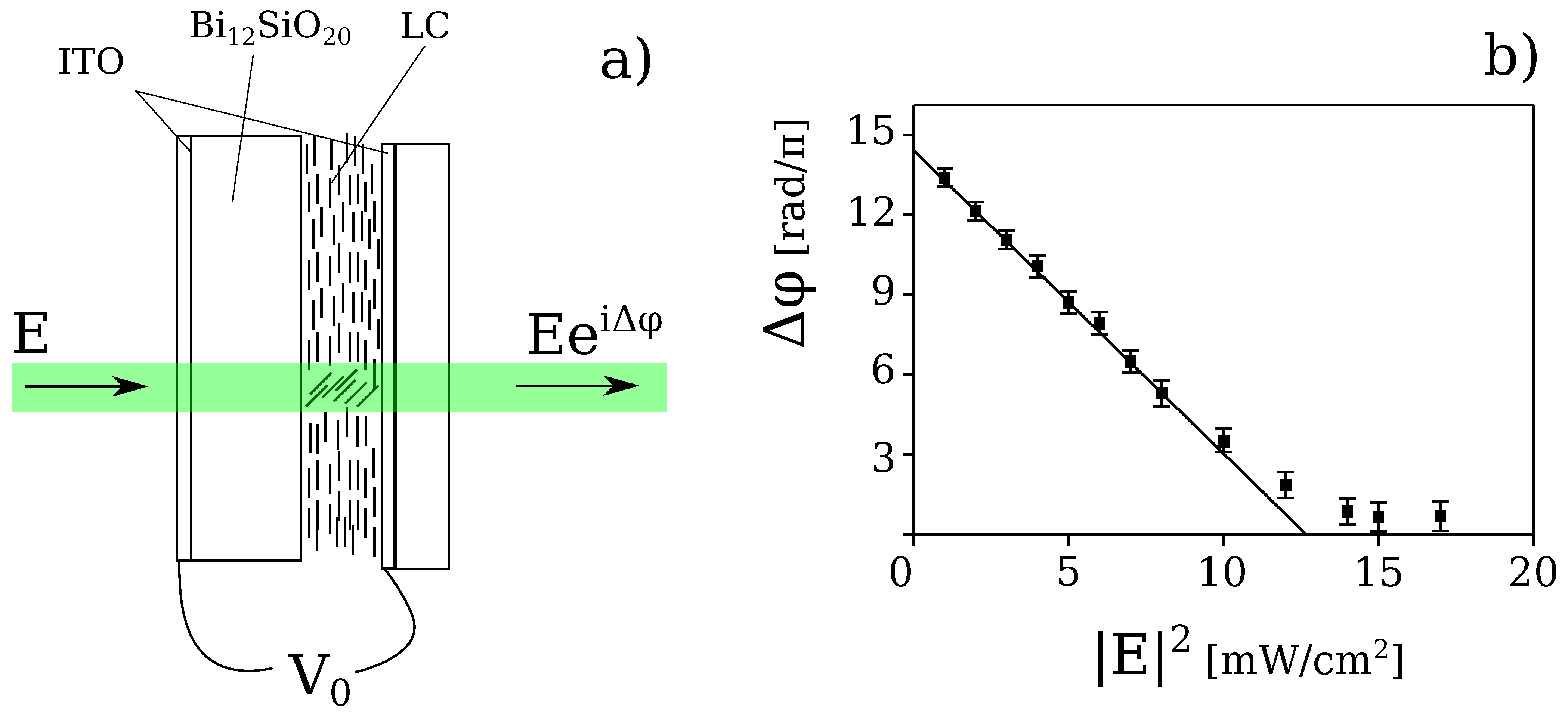
The liquid crystal light-valve is schematically depicted in Figure 1a. It is made by associating a liquid crystal (LC) layer with a photorefractive (BSO) crystal, cut in the form of a thin plate (1 thickness, 20 × 30 lateral size) [19,21]. The BSO is one of the confining wall and the other wall is a glass window. The thickness of the LC layer is typically of the order of 10 . While liquid crystals are used for their large birefringence, the BSO is used for its large photoconductivity and transparency in the visible range [11]. Transparent electrodes (Indium Tin Oxide, ITO, layers) deposited over the BSO and the glass wall allow the application of an external voltage across the LC layer. The voltage applied is AC, with a rms value from 2 to 20 V and a frequency from 50 to 20 . The liquid crystals are nematics E48 (from Merck).
Figure 1.
(a) Schematic representation of the liquid crystal light-valve; (b) Measured phase shift as a function of the input intensity .
Figure 1.
(a) Schematic representation of the liquid crystal light-valve; (b) Measured phase shift as a function of the input intensity .

The nematic phase is characterized by a long range orientational order for which all the molecules are aligned, in average, along a preferential direction, so called the nematic director [29]. Because the molecules have a different polarizability along their long and short axis, and being the dielectric susceptibility parallel, respectively, orthogonal to the long axis of the molecules, when an electric field, or a voltage , is applied across the nematic layer, an induced dipole moment arises and all the molecules reorient towards the direction of the applied field.
Because of the LC birefringence, the nematic layer as a whole behaves like a strongly birefringent material, characterized by a different refractive index for a beam polarized along the long or short molecular axis, called, respectively, the extraordinary and the ordinary index. Typical values for nematics are and , which gives birefringence as large as . Therefore, when the LC molecules reorient under the action of an applied field, their collective motion implies a change of the principal axis of the nematic layer, hence, an incoming light field experiences a corresponding refractive index change [30]. When a light beams impinges onto the LCLV, photo-generation of charges occurs at the BSO surface because of its photoconductive properties. Therefore, the local voltage across the LC layer increases, inducing a further molecular reorientation and thus an additional refractive index change. As a result, at the exit of the LCLV, the light beam acquires a phase shift that is a function of the applied voltage and of the total intensity of the incident beam.
A typical characteristic of the LCLV is shown in Figure 1b. The phase shift measured on the output beam is plotted as a function of the input intensity , where E is the amplitude of the incident light beam. In the linear region of its response, the LCLV behaves as a Kerr-like nonlinear medium, providing a refractive index change proportional to the input light intensity , where is the value fixed by the applied voltage and the nonlinear coefficient. Saturation occurs when all the LC molecules are aligned along the direction of the applied electric field. Thanks to the large LC birefringence, the nonlinear coefficient, which is the slope of the linear part of the response curve, is as large as , the minus sign accounting for the defocusing character of the nonlinearity (the refractive index changes from to , with when LC molecules reorient under the action of the electric field).
The response time is dictated by the time required by the collective motion of the LC molecules to establish over the whole thickness d of the nematic layer. This is given by
where γ is the LC rotational viscosity and K the splay elastic constant [29]. For and typical values of the LC constants, is of the order of 100 . The spatial resolution, which is the minimal size of an independently addressed area, is given by the electric coherence length of the LC
where is the dielectric anisotropy of the LC. For the usual values of , is typically of the order of 10 .
3. Two-Wave Mixing in the LCLV
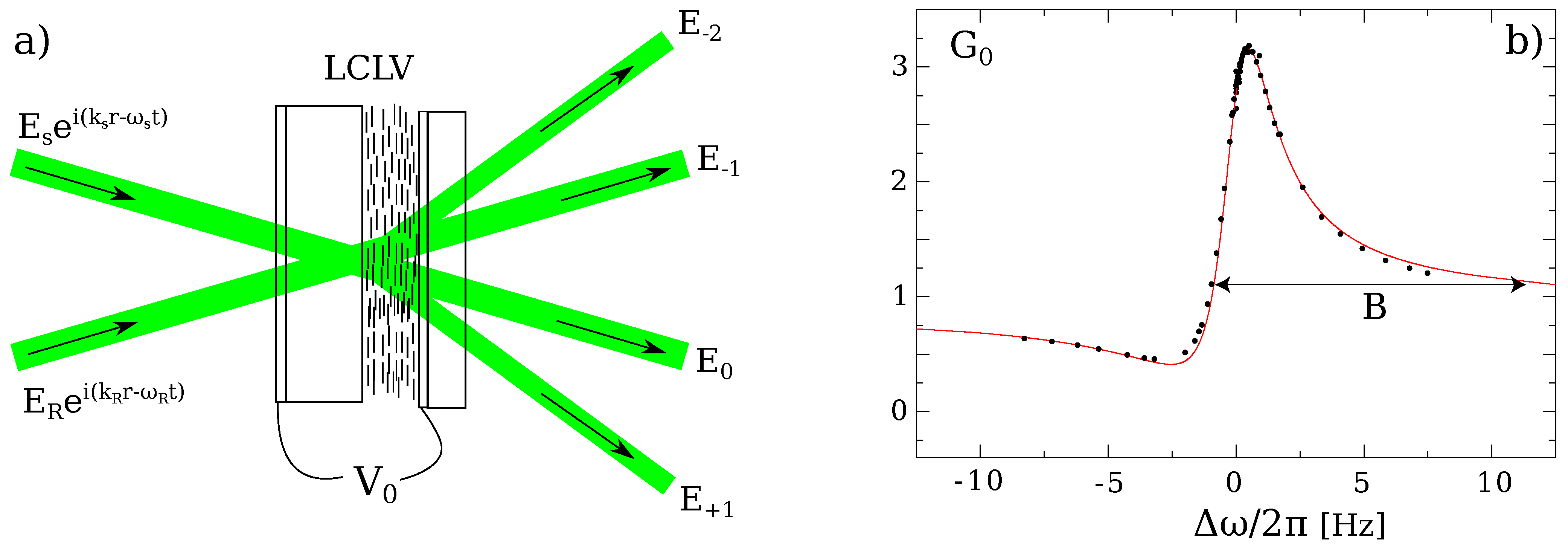
In the LCLV the active medium is the LC layer that is usually thin (of the order of 10 ) when compared to the typical fringe spacing (of the order of 100 ). Therefore, when two-wave mixing is performed in the LCLV, the beam coupling occurs in the Raman–Nath regime of diffraction. Different from the Bragg regime, for which the phase matching condition is satisfied only in one direction, the Raman–Nath diffraction produces several output order beams [31]. The interaction scheme comprises a reference beam , which is sent onto the LCLV together with a signal beam , as depicted in Figure 2a. The total electric field at the input of the LCLV can be written as
where and are the amplitudes of the reference, respectively, the signal waves, and their respective propagation vectors and , their frequencies. The two beams produce an intensity fringe pattern
where is the total input intensity, is the grating wave vector and the frequency detuning between the reference and signal. The ratio between the reference and signal intensity is usually kept much larger than one.
Figure 2.
(a) Two-wave mixing in the liquid crystal light-valve; (b) Measured (points) and theoretical (line) gain as a function of the frequency detuning between the reference and signal beam. B is the frequency bandwidth characterizing the two-beam coupling process.
Figure 2.
(a) Two-wave mixing in the liquid crystal light-valve; (b) Measured (points) and theoretical (line) gain as a function of the frequency detuning between the reference and signal beam. B is the frequency bandwidth characterizing the two-beam coupling process.

The fringe pattern induces, on its turn, a photo-induced space charge distribution, hence a molecular reorientation pattern in the LC layer, which creates a refractive index grating with the same wave vector . The spatial period of the grating is usually larger than the thickness of the LC layer. Therefore, the LC grating acts as a thin hologram, and several diffracted beams, distinguished by the numbers , are observed at the output of the LCLV. Due to self-diffraction, photons from the pump are transferred into the different output orders. The orders are amplified; that is, they receive from the reference, also called pump beam, more photons than they are losing due to the scattering on the other orders. The order is the reference beam that, even though depleted, remains of much higher intensity than the other beams [32].
To derive the full expression for the output field, we have to consider the evolution of the amplitude of the refractive index grating inside the LC layer. This is governed by a relaxation equation following the molecular orientation dynamics of the LC [29]
where is the transverse diffusion length, is the constant value of the refractive index given by the average LC orientation under the application of the voltage , and is the equivalent Kerr-like coefficient of the LCLV. By coupling the above Equation (5) with the wave propagation equation for the input electric field, one can easily shows that the m output order field can be written as [32,33,34]
where is the frequency, the wave vector and the amplitude is given by
where is the Bessel function of the first kind and of order m,
is the grating amplitude and
from the above expression Equation (7), we see that each order m receive two contributions, one is the scattering of the signal and the other is the scattering of the reference beam onto the refractive index grating.
It is useful to write each output order field in the form
where we define as the gain factor and is the associated nonlinear phase shift. Both and can be calculated from Equation (7).
Let us consider the order, which coincides with the original propagation direction of the signal
The envelope amplitude can also be written as
where is the total input intensity. The two contributions, namely the scattering of the signal and the scattering of the reference beam, sum up with their relative phases. The final effect is to produce a gain with a narrow frequency bandwidth. In Figure 2b, the gain curve is plotted as a function of the frequency detuning for parameter values close to typical experimental conditions, , , , , and and compared with the experimental data (filled circles). The maximum gain (and, correspondingly, maximum phase shift) is obtained for . In correspondence, a temporally modulated signal will experience a large dispersion, due to the strong selectivity of the gain whose frequency bandwidth is approximately .
4. LCLV-Based Adaptive Holography: Setup and Theoretical Background
Adaptive holography interferometry, AHI, is realized in the LCLV by performing two-wave mixing experiments as described above. The narrow frequency bandwidth of the gain and the high nonlinear response of the LCLV, allowing its operation at low light powers, makes the LCLV an ideal medium for adaptive holography [35]. In a similar way as it occurs for AHI in photorefractive crystals [5], the gain resonance curve acts as an optical filter able to adapt the dynamic hologram by following low frequency variations and noise disturbances (inside the two-wave mixing gain bandwidth B).
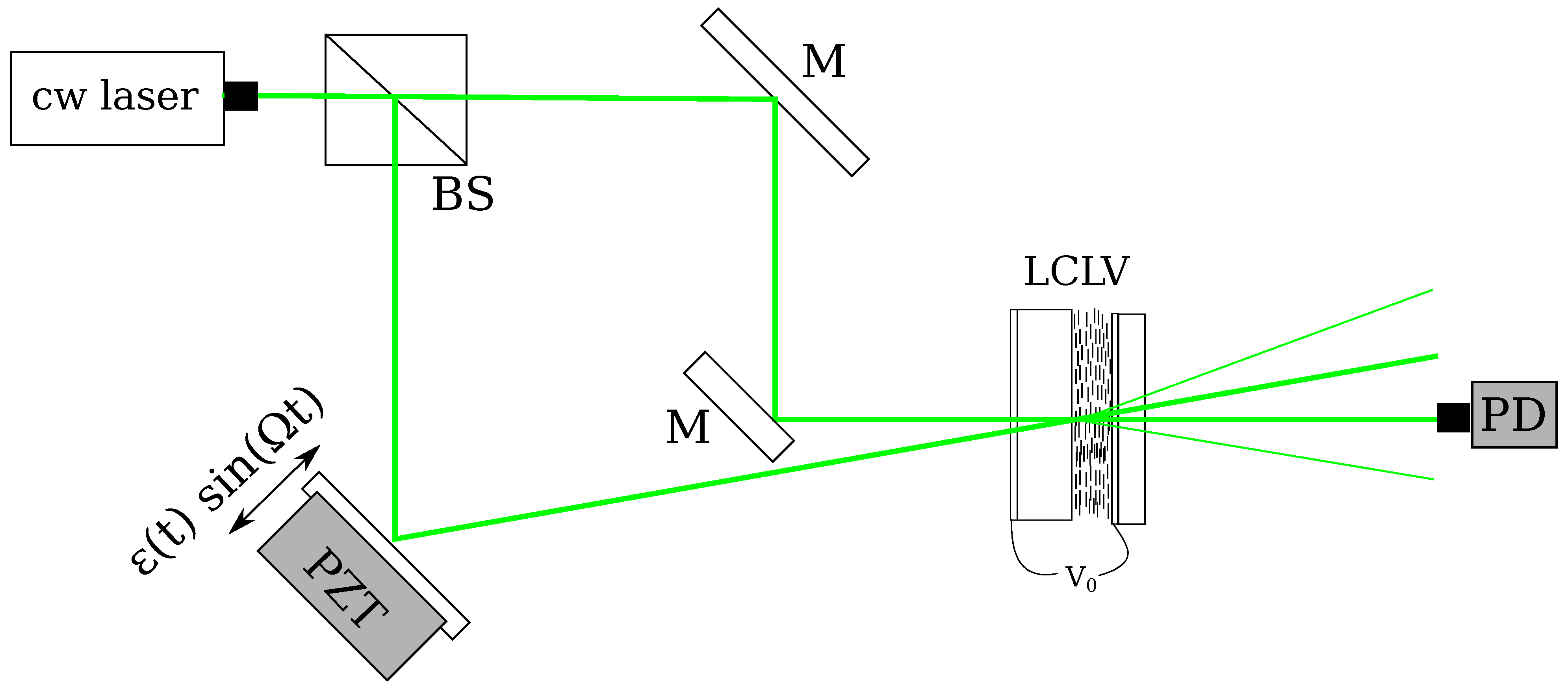
The experimental setup for AHI in the LCLV is shown in Figure 3. The input beam is from a cw doubled diode-pumped solid-state laser, wavelength 532 , with the total input intensity typically less than 5 . The laser beam is divided into a reference and a signal wave. By means of a piezoelectrically driven mirror the signal beam is phase modulated with a sinusoidal oscillation at high frequency and small amplitudes ε. The signal beam is sent onto the LCLV together with the reference beam , thus producing a thin diffraction grating. Several output beams are obtained at the exit of the LCLV. The optical power of the output beams is measured with a photodiode and a lock-in amplifier.
Figure 3.
Experimental setup of the AHI interferometer with the LCLV as adaptive hologram. The input laser is split into a reference and a signal beams that are incident on the LCLV; before arriving at the LCLV the signal is sent to a vibrating object, whose amplitude of oscillation we want to detect. PZT, piezoelectrically driven mirror. The output intensity on the −1 order is measured with a photodiode PD and converted to a voltage.

The frequency of the modulation Ω is much greater than the bandwidth B of the two-wave-mixing in the LCLV. The total intensity distribution on the LCLV is
where is the laser frequency, is the phase shift due to the vibrating object, is the small displacement that we aim to detect, χ is the incidence angle of the light beam on the vibrating surface, and Δ is the optical path difference acquired by the reference and signal before arriving at the LCLV.
Given the narrow frequency bandwidth of the gain, the grating formation automatically filters out the high frequency and the amplitude of the phase grating reads as [36]
Because of the large value of the LCLV nonlinear coefficient , the process is very efficient and the output diffracted beams are easily detected. By solving the wave propagation equation in the Raman–Nath regime [35], we obtain for the optical power of the m output order
where is the total absorption coefficient of the LCLV, the thickness of the photoconductor, the ratio between the signal and reference power and the Bessel function of the first kind and of order m. By substituting in Equation (15) the expression for θ, we find the component at the modulation frequency Ω
where we have made use of the component parts of the Fourier–Bessel expansion [37]. Either the zero order beam, which coincides with the direction of the signal, or the beam, which coincides with the direction of the reference, is detected with a photodiode and a lock-in amplifier. These orders are also used to calibrate the system. Indeed, if and for we have
which has a maximum at . As already done in other AHI setups [38,39], this property has been used to find the relation between the displacement ε and the measured lock-in voltage .
4.1. Relative Detection Limit
For small displacements we can approximate and the detection becomes linear with ε, which automatically gives the highest sensitivity of the AHI interferometer. In classical interferometers, to achieve this condition the average phase difference between the interfering beams has to be set to (quadrature condition). Moreover, the AHI system does not require the stabilization with respect to variations of the optical path difference Δ, since the beam coupling is self-adapted. The sensitivity of the AHI system is obtained by considering the limit given by the photon shot-noise. The signal to noise ratio in this case can be expressed as [7,35]
where η is the quantum efficiency of the photodiode and is the bandwidth of the electronic detection system. The minimum detectable displacement is calculated by setting SNR. In order to compare the performances of the AHI with classical homodyne detection, the relative detection limit has to be considered. In the case of a classical interferometer in quadrature configuration and lossless, the ideal detection limit is [7]
thus, we obtain
the minimum is obtained for the order. Correspondingly, the maximum signal to noise ratio is obtained and the minimum detectable phase is of the order of 7 .
5. Experimental Results: Picometer Detection
The typical experimental setup for AHI with the LCLV is displayed in Figure 3. In the following set of measurements the frequency of the modulation was fixed at , which is much greater than the bandwidth of the two-wave-mixing in the LCLV. A photodiode () was placed on one of the diffracted orders and the output optical power was measured by using a lock-in amplifier (1 bandwidth). The signal was detected at the order, for which the theoretical curves predict the maximum sensitivity. The data are plotted in Figure 4a as a function of the mirror displacement ε. The intensity of the signal beam was 3 and .
Figure 4.
(a) Linear and (b) log scale plot of the signal detected at the output of the LCLV (−1 order) versus the mirror displacement ε; frequency of modulation , , , ; the solid curves are the fits with the theoretical curve . From Reference [35].
Figure 4.
(a) Linear and (b) log scale plot of the signal detected at the output of the LCLV (−1 order) versus the mirror displacement ε; frequency of modulation , , , ; the solid curves are the fits with the theoretical curve . From Reference [35].
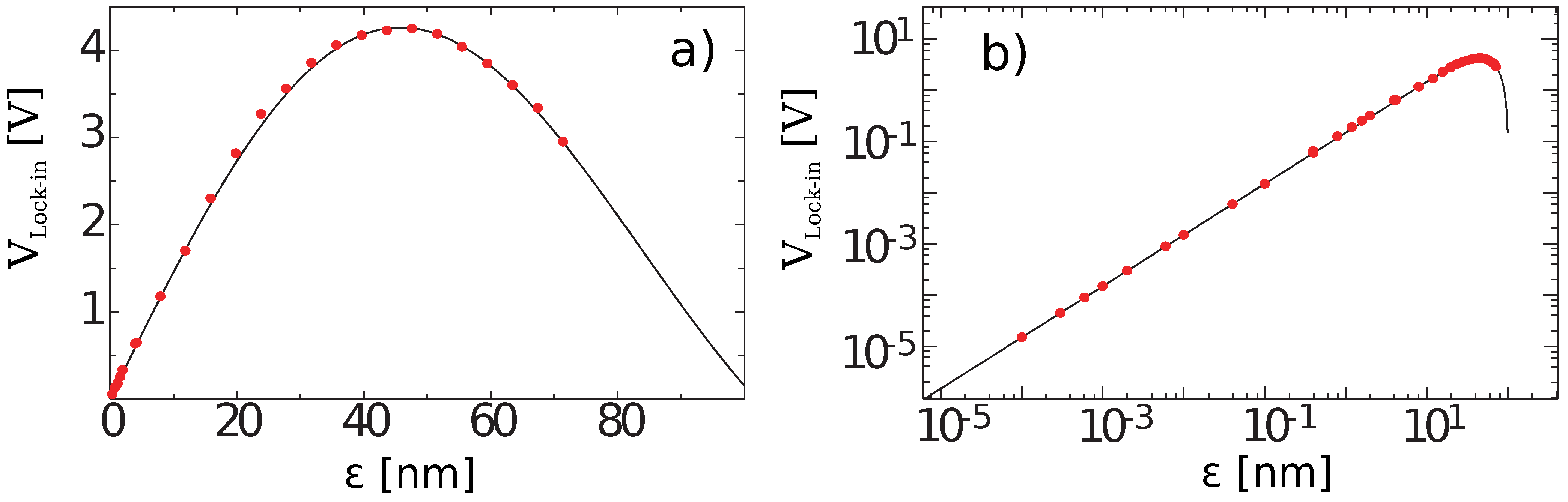
In Figure 4b the same data as in Figure 4a are plotted in logarithmic scale, from which it can be clearly seen that for small displacements the detection is linear. Mirror displacements as small as are efficiently detected. Similar results can be obtained on the zero order. The theoretical detection limit is not reached, mainly because the smallest displacement that could be achieved was limited by the sensitivity of the vibrating system. The ultimate relative detection limit, theoretically predicted to be times that of an ideal interferometer, could be reached in future by using more sophisticated electronics and better isolated working conditions.
5.1. Pressure Radiation Measurements
It is well known that the pressure P of normally incident cw light experienced by a macroscopic object with a plane surface has a linear dependence on the light intensity I
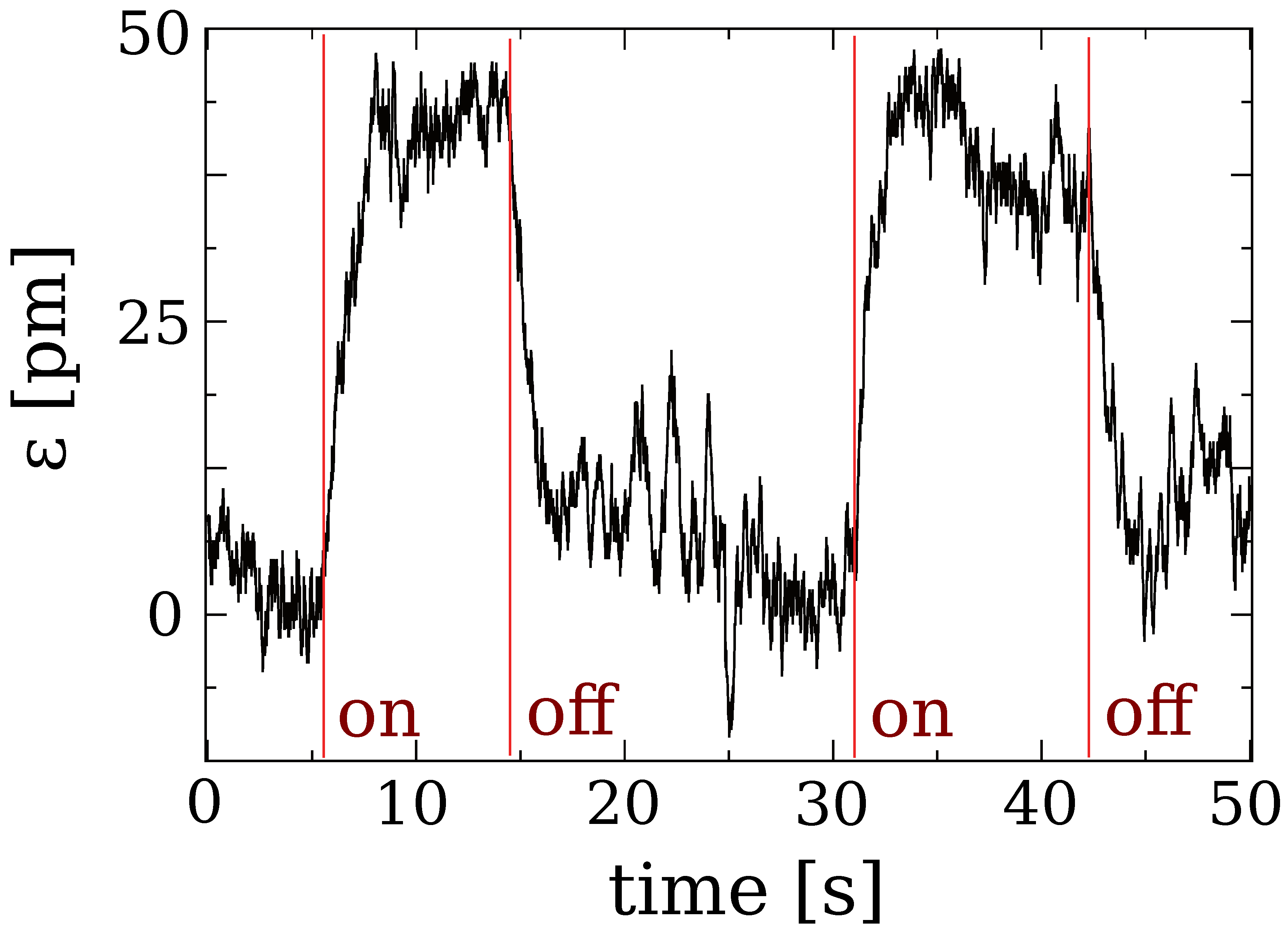
where c is the speed of light and R is the reflectivity of the illuminated surface of the object. It was demonstrated by using a photorefractive crystal that AHI is an efficient tool to measure light pressure radiation [39]. Successive experiments have demonstrated the ability of AHI to detect light radiation pressure by using the LCLV. The setup is similar to that depicted in Figure 3. A 5 thick nitrocellulose membrane with a reflective coating was used as a vibrating object. The membrane was placed inside a vacuum box in order to reduce air pressure perturbations. A laser beam with power 45 , and waist 3 impinged on the rear side of the membrane. The laser was square modulated at a frequency 10 and could be switched on/off by external control.
The detected signal reflected by the membrane is shown in Figure 5. The laser-induced displacement can be clearly detected. The transition rate of 1 is due to the bandwidth of the lock-in, whereas the noise is related to fluctuations of the membrane under the laser-induced deformation and subsequent relaxation.
Figure 5.
Laser-induced membrane displacement; on/off indicates the state of the laser.

5.2. Multimode Fiber: Acoustic Detection
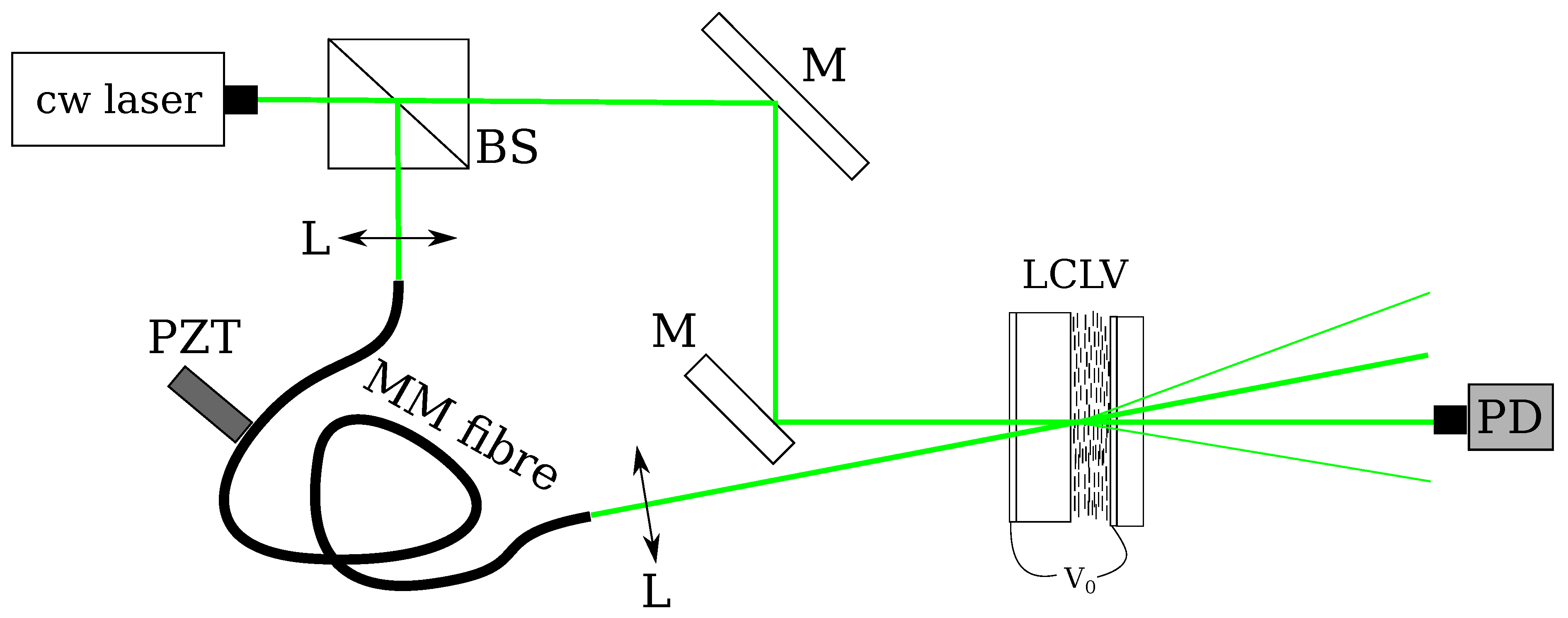
In order to test the ability of the LCLV to work with complex wavefronts, we have performed AHI by taking as signal the optical field distribution at the exit of a multimode fiber. The setup is sketched in Figure 6. A high frequency modulation is created by sending on the fiber an acoustic wave at through a piezoelectric transducer. Low frequency perturbations are induced by local, and small, disturbances, induced, for example, by touching the fiber. At the exit of the fiber, the optical field distribution has a speckle pattern with a slow dynamics.
Figure 6.
(color online). Schematic setup for the detection of phase modulations of a speckle field at the exit of a multimode fiber, MM. PZT is a piezoelectric transducer modulating in contact with the multimode fiber.
Figure 6.
(color online). Schematic setup for the detection of phase modulations of a speckle field at the exit of a multimode fiber, MM. PZT is a piezoelectric transducer modulating in contact with the multimode fiber.

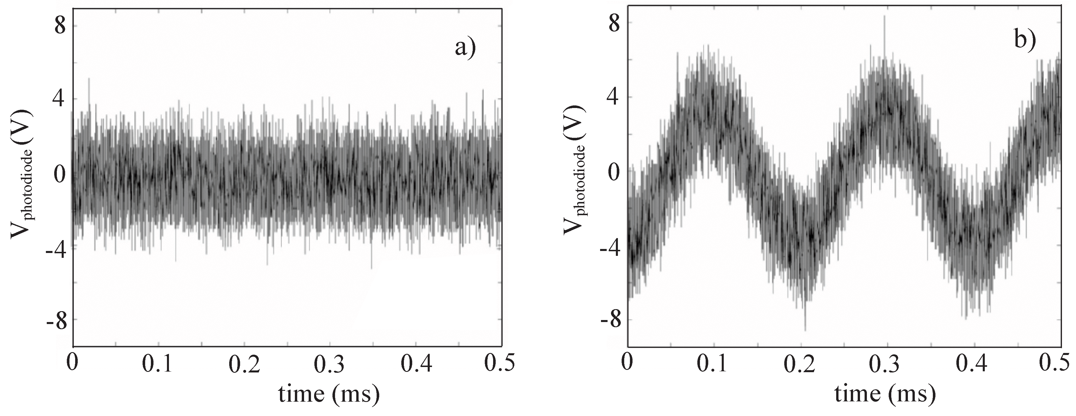
In the case of a classical interferometer the phase modulations of the signal are completely hidden by the noise, as shown in Figure 7a. In the case of AHI, the two-wave mixing in the LCLV provides a narrow frequency bandwidth that filters out low frequency noise fluctuations, and the acoustic wave modulating the signal can be clearly distinguished. This is evident in Figure 7b, which plots the time evolution of the photodiode signal measured after the LCLV in the adaptive interferometer setup.
Figure 7.
(color online). Signal detected as a function of time in the case of (a) a Michelson interferometer and (b) after the LCLV in the AHI system.
Figure 7.
(color online). Signal detected as a function of time in the case of (a) a Michelson interferometer and (b) after the LCLV in the AHI system.
6. Conclusions
Nonlinear optical interactions can be efficiently implemented in liquid crystal light-valves by performing wave-mixing experiments. Optical beam amplification is obtained via two-wave mixing and a narrow frequency bandwidth is associated to the resonant character of the two-beam coupling process. This property can be exploited to realize self-adaptive interferometric systems that have been demonstrated efficient for the detection of displacements as small as fractions of picometers. Moreover, the self-adaptive character of the nonlinear process allows to perform phase detection with spatially complex wavefronts, such as speckles or distorted fields, and to detect acoustic waves in noisy environment.
Acknowledgments
U.B. and S.R. acknowledge financial support of the ANR ASTRID program, project ANR- 11-ASTR-0012, MEDUSE.
References
- Petrov, M.P. Introduction to Optical Signal Processing with Photorefractive Materials; Gunter, P., Ed.; Springer-Verlag: New York, NY, USA, 1987; pp. 284–290. [Google Scholar]
- Petrov, M.P.; Stepanov, S.I.; Khomenko, A.V. Photorefractive Crystals in Coherent Optical Systems; Springer: Berlin, Germany, 1991. [Google Scholar]
- Kamshilin, A.A.; Petrov, M.P. Continuous reconstruction of holographic interferograms through anisotropic diffraction in photorefractive crystals. Opt. Commun. 1985, 53, 23–25. [Google Scholar] [CrossRef]
- Petrov, M.P.; Petrov, V.M.; Zouboulis, I.S.; Xu, L.P. Two-wave and induced three-wave mixing on a thin Bi12TiO20 hologram. Opt. Commun. 1997, 134, 569–579. [Google Scholar] [CrossRef]
- Kamshilin, A.A.; Romashko, R.V.; Kulchin, Y.N. Adaptive interferometry with photorefractive crystals. J. Appl. Phys. 2009, 105, 031101:1–031101:11. [Google Scholar] [CrossRef]
- Petrov, V.; Denz, C.; Petter, J.; Tschudi, T. Enhancing the sensitivity of an adaptive holographic interferometer using non-Bragg diffraction orders. Opt. Lett. 1997, 22, 1902–1904. [Google Scholar] [CrossRef] [PubMed]
- De Montmorillon, L.A.; Delaye, P.; Launay, J.C.; Roosen, G. Novel theoretical aspects on photorefractive ultrasonic detection and implementation of a sensor with an optimum sensitivity. J. Appl. Phys. 1997, 82, 5913–5922. [Google Scholar] [CrossRef]
- Kamshilin, A.A.; Grachev, A.I. Adaptive interferometer based on wave mixing in a photorefractive crystal under alternating electric field. Appl. Phys. Lett. 2002, 81, 2923–2925. [Google Scholar] [CrossRef]
- Di Girolamo, S.; Kamshilin, A.A.; Romashko, R.V.; Kulchin, Y.N.; Launay, J.C. Fast adaptive interferometer on dynamic reflection hologram in CdTe:V. Opt. Exp. 2006, 15, 545–555. [Google Scholar] [CrossRef]
- Lesaffre, M.; Jean, F.; Ramaz, F.; Boccara, A.C.; Gross, M.; Delaye, P.; Roosen, G. In situ monitoring of the photorefractive response time in a self-adaptive wavefront holography setup developed for acousto-optic imaging. Opt. Exp. 2007, 15, 1030–1042. [Google Scholar] [CrossRef]
- Gunter, P.; Huignard, J.P. Photorefractive Materials and their Applications 1, 2 and 3; Springer: New York, NY, USA, 2006. [Google Scholar]
- Efron, U.; Liverscu, G. Spatial Light Modulator Technology: Materials, Devices and Applications; Dekker: New York, NY, USA, 1995. [Google Scholar]
- Collings, N. Optical Pattern Recognition Using Holographic Techniques; Addison-Wesley: Reading, MA, USA, 1998. [Google Scholar]
- Armitage, D.; Thackara, J.I.; Eades, W.D. Photoaddressed liquid crystal spatial light modulators. Appl. Opt. 1998, 28, 4763–4771. [Google Scholar] [CrossRef] [PubMed]
- Grinberg, J.; Jacobson, A.; Bleha, W.; Miller, L.; Fraas, L.; Boswell, D.; Myer, G. A new real-time non-coherent to coherent light image converter—The hybrid field effect liquid crystal light valve. Opt. Eng. 1975, 14, 217–225. [Google Scholar] [CrossRef]
- Ashley, P.R.; Davis, J.H. Amorphous silicon photoconductor in a liquid crystal spatial light modulator. Appl. Opt. 1978, 26, 241–246. [Google Scholar] [CrossRef] [PubMed]
- Akhmanov, S.A.; Vorontsov, M.A.; Ivanov, V. Iu. Large-scale transverse nonlinear interactions in laser beams–New types of nonlinear waves, onset of “optical turbulence". JETP Lett. 1988, 47, 707–711. [Google Scholar]
- Efron, U.; Wu, S.T.; Bates, T.D. Nematic liquid crystals for spatial light modulators: Recent studies. J. Opt. Soc. Am. B 1986, 3, 247–252. [Google Scholar] [CrossRef]
- Aubourg, P.; Huignard, J.P.; Hareng, M.; Mullen, R.A. Liquid crystal light valve using bulk monocrystalline Bi12SiO20 as the photoconductive material. Appl. Opt. 1982, 21, 3706–3712. [Google Scholar] [CrossRef] [PubMed]
- Sanner, N.; Huot, N.; Audouard, E.; Larat, C.; Huignard, J.P.; Loiseaux, B. Programmable focal spot shaping of amplified femtosecond laser pulses. Opt. Lett. 2005, 30, 1479–1481. [Google Scholar] [CrossRef] [PubMed]
- Brignon, A.; Bongrand, I.; Loiseaux, B.; Huignard, J.P. Signal-beam amplification by two-wave mixing in a liquid-crystal light valve. Opt. Lett. 1997, 22, 1855–1857. [Google Scholar] [CrossRef] [PubMed]
- Bortolozzo, U.; Residori, S.; Petrosyan, A.; Huignard, J.P. Pattern formation and direct measurement of the spatial resolution in a photorefractive liquid crystal light valve. Opt. Commun. 2006, 263, 317–321. [Google Scholar] [CrossRef]
- Bortolozzo, U.; Residori, S.; Huignard, J.P. Enhancement of the two-wave-mixing gain in a stack of thin nonlinear media by use of the Talbot effect. Opt. Lett. 2006, 31, 2166–2168. [Google Scholar] [CrossRef] [PubMed]
- Residori, S.; Bortolozzo, U.; Huignard, J.P. Slow light using wave mixing in liquid crystal light valve. Appl. Phys. B 2009, 95, 551–557. [Google Scholar] [CrossRef]
- Residori, S.; Bortolozzo, U.; Huignard, J.P. Slow and fast light in liquid crystal light valves. Phys. Rev. Lett. 2008, 100, 203603:1–203603:4. [Google Scholar] [CrossRef] [PubMed]
- Bortolozzo, U.; Residori, S.; Huignard, J.P. Slow-light birefringence and polarization interferometry. Opt. Lett. 2010, 35, 2076–2078. [Google Scholar] [CrossRef] [PubMed]
- Bortolozzo, U.; Residori, S.; Rubin, J.; Huignard, J.P. Sagnac interferometer with adaptive nonlinear detection. Opt. Lett. 2011, 36, 520–522. [Google Scholar] [CrossRef] [PubMed]
- Lenzini, F.; Residori, S.; Arecchi, F.T.; Bortolozzo, U. Optical vortex interaction and generation via nonlinear wave mixing. Phys. Rev. A 2011, 84, 061801:1–061801:4. [Google Scholar] [CrossRef]
- De Gennes, P.G.; Prost, J. The Physics of Liquid Crystals; Oxford Science Publications: Clarendon, TX, USA, 1993. [Google Scholar]
- Khoo, I.C. Liquid Crystals: Physical Properties and Nonlinear Optical Phenomena, 2nd ed.; Wiley Interscience: New York, NY, USA, 2007. [Google Scholar]
- Yariv, A. Optical Waves in Crystals; John Wiley & Sons: Hoboken, NJ, USA, 2003; pp. 354–358. [Google Scholar]
- Bortolozzo, U.; Residori, S.; Huignard, J.P. Tuning the group delay of optical wave packets in liquid-crystal light valves. Phys. Rev. A 2009, 79, 053835:1–053835:9. [Google Scholar] [CrossRef]
- Bortolozzo, U.; Residori, S.; Huignard, J.P. Slow and fast light: Basic concepts and recent advancements based on nonlinear wave-mixing processes. Laser Photonics Rev. 2010, 4, 483–498. [Google Scholar] [CrossRef]
- Bortolozzo, U.; Residori, S.; Huignard, J.P. Adaptive holography and slow-light in liquid-crystal light-valves. J. Hologr. Speckles 2009, 5, 1–8. [Google Scholar] [CrossRef]
- Bortolozzo, U.; Residori, S.; Huignard, J.P. Picometer detection by adaptive holographic interferometry in a liquid-crystal light valve. Opt. Lett. 2009, 34, 2006–2008. [Google Scholar] [CrossRef] [PubMed]
- Huignard, J.P.; Marrakchi, A. Two-wave mixing and energy transfer in Bi12SiO20 crystals: Application to image amplification and vibration analysis. Opt. Lett. 1981, 6, 622–624. [Google Scholar] [CrossRef] [PubMed]
- Wagner, J.W.; Spicer, J.B. Theoretical noise-limited sensitivity of classical interferometry. J. Opt. Soc. Am. B 1987, 4, 1316–1326. [Google Scholar] [CrossRef]
- Petrov, V.; Denz, C.; Petter, J.; Tschudi, T. Enhancing the sensitivity of an adaptive holographic interferometer using non-Bragg diffraction orders. Opt. Lett. 1997, 22, 1902–1904. [Google Scholar] [CrossRef] [PubMed]
- Petrov, V.; Hahn, J.; Petter, J.; Petrov, M.; Tschudi, T. Precise subnanometer control of the position of a macro object by light pressure. Opt. Lett. 2005, 30, 3138–3140. [Google Scholar] [CrossRef] [PubMed]
© 2012 by the authors; licensee MDPI, Basel, Switzerland. This article is an open access article distributed under the terms and conditions of the Creative Commons Attribution license (http://creativecommons.org/licenses/by/3.0/).
Share and Cite
MDPI and ACS Style
Bortolozzo, U.; Residori, S.; Huignard, J.-P. Adaptive Holography in Liquid Crystal Light-Valves. Materials 2012, 5, 1546-1559. https://doi.org/10.3390/ma5091546
AMA Style
Bortolozzo U, Residori S, Huignard J-P. Adaptive Holography in Liquid Crystal Light-Valves. Materials. 2012; 5(9):1546-1559. https://doi.org/10.3390/ma5091546
Chicago/Turabian StyleBortolozzo, Umberto, Stefania Residori, and Jean-Pierre Huignard. 2012. "Adaptive Holography in Liquid Crystal Light-Valves" Materials 5, no. 9: 1546-1559. https://doi.org/10.3390/ma5091546