Fuel Economy Improvement of a Heavy-Duty Powertrain by Using Hardware-in-Loop Simulation and Calibration

Abstract

Fuel economy efficiency is one of the most important parameters for vehicle powertrains, which is of particular interest for heavy-duty powertrain calibration. Conventionally, this work relies heavily on road tests, which cost more and may lead to long duration product development cycles. The paper proposes a novel hardware-in-loop modeling and calibration method to work it out. A dSPACE hardware-based test bench was successfully established and validated, which is valuable for a more efficient and easier shift schedule in calibration. Meanwhile, a real-time dynamic powertrain model, including a diesel engine, torque converter, gear box and driver model was built. Typical driving cycles that both velocity and slope information were constructed for different road conditions. A basic economic shift schedule was initially calculated and then optimal calibrated by the test bench. The results show that there is an optimal relationship between an economic shift schedule and speed regulation. By matching the best economic shift schedule regulation to different road conditions; the fuel economy of vehicles can be improved. In a smooth driving cycle; when the powertrain applies a larger speed regulation such as 12% and the corresponding shift schedule; the fuel consumption is smaller and is reduced by 13%. In a complex driving cycle, when the powertrain applies a smaller speed regulation such as 5% along with the corresponding shift schedule; the fuel consumption is smaller and is reduced by 5%. The method thus can provide guidance for economic calibration experiments of off-road heavy-duty vehicles.

1. Introduction

Vehicles with good fuel economy can reduce the operating cost of vehicles, reduce a country’s dependence on importing oil, save oil resources and reduce engine emissions [1]. The standard methods of measuring fuel economy are the constant velocity fuel consumption test and driving cycle fuel consumption test [2]. The first method measures a vehicle’s fuel consumption when the vehicle runs 100 km in the highest gear on a good road and under a certain load. However, the constant velocity driving cycle cannot comprehensively reflect the actual operation of the vehicle. Based on tracking, measurements and statistics of actual vehicles, many countries have established some typical driving cycles to simulate the real vehicle running status [3]. The most popular driving cycles are the American driving cycle, European driving cycle and Japanese driving cycle. Among them FTP (Federal Test Program) of America and ECE (Economic Commission for Europe) of Europe are used more widely [4].

In the American FTP75, vehicles run 2475 s. The highest velocity is 91.2 km/h and average velocity is 31.4 km/h. In order to revise FTP, researchers have developed many driving cycles to reflect more realistic traffic conditions, and the main achievements were some supplementary versions of the FTP. The FTP has been applied to vehicle emission tests of production vehicles since 2001 and the highway cycle is applied to vehicles running on the highway [5].

Europe is applying the ECE + European Urban Driving Cycle (EUDC) at present. The ECE + EUDC can be divided into two parts. The first part is a traditional urban driving cycle which consists of 15 driving modes. In the driving cycle, vehicles are tested for 780 s and its distance is 4.052 km and average velocity is 18.7 km/h. The second part is a suburban driving cycle that reflects suburban vehicle driving conditions. In this driving cycle, vehicles are tested for 400 s and the distance is 6.955 km. The highest velocity is 120 km/h and the average velocity is 62.6 km/h. To develop new power vehicles, European researchers have studied many driving cycles, the most famous work of which is Modem-hyzem [6].

Before 1991 Japan applied the Japan 10 test, which reflects vehicle driving conditions in city center areas. Japan 11 reflects vehicle driving conditions from suburban to urban or in the suburban area. By modifying Japan 10, Japan established Japan10–15 due to the changes to the urban structure and traffic flow. In the driving cycle, vehicles are tested for 460 s, the highest velocity is 70 km/h and the average velocity is 22.7 km/h [7].

Divided according to the different experimental places used, methods of measuring the vehicle fuel economy can be road tests and bench tests, both of which have shortcomings of high test costs and long test periods, etc. Besides, the results may not be accurate because the bench test method cannot simulate rolling resistance, air resistance and inertia resistance accurately. Meanwhile, as discussed by Sun [8], an optimal relationship between economic shift schedule and speed regulation exists for the best economic performances, which tends to be a new spotlight in this field of study. For these reasons, this paper puts forward a new method of virtual calibration of an economic shift schedule for heavy-duty vehicle powertrains based on a typical driving cycle and applies hardware-in-the-loop simulation.

By bringing the mathematical optimization theory into the parameter calibration of the engine electronic control system, it guarantees the engine achieves the highest efficiency while satisfying certain constraints. This method which uses experimental data to fit the model and carry out parameter optimization is also based on the model calibration technology [9].

As the electronic control units (ECU) in vehicles become more complex, the calibration requirements are also increasing, and the development of automatic test technique provides new space for development of the calibration techniques. Automated tests can significantly reduce the test time and can acquire many test points, allowing engineers to get a clear image to understand the characteristics of the engine [10]. The leading companies in the automatic calibration field are AVL in Austria and SCHENCK in Germany. For the automatic calibration system, the AVL uses the software CAMEO as its kernel and the SCHENCK equipment uses the software VEGA as the kernel, both of which are based on the Association for Standardization of Automation and Measuring Systems (ASAM) platform. In recent years, many researchers have used AVL CAMEO to run intelligent engine calibration to minimize the testing effort on the basis of the Design of Experiment approach [11,12,13]. Meanwhile, in this paper the dSPACE system is chosen as the virtual calibration platform. Compared with other calibration systems, it is easier to operate and has greater functionality.

2. Methods

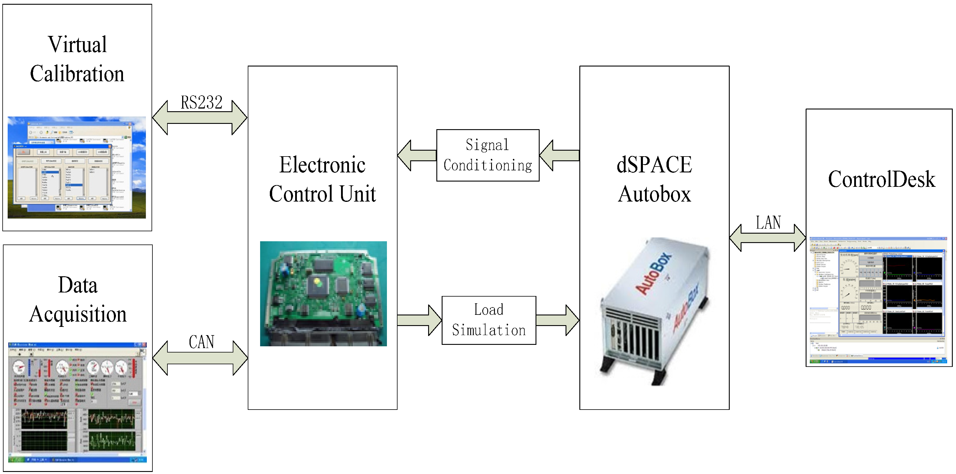
2.1. Virtual Calibration Platform

The dSPACE system is a development and testing platform based on a MATLAB/Simulink control system. It can connect seamlessly with MATLAB/Simulink. The dSPACE real-time system has a hardware system of high speed calculation ability (including CPU, I/O, etc.), so as to generate or download real-time code conveniently and has a software environment for experiments and debugging as discussed by Li [14]. This paper applies the hardware-in-the-loop simulation platform based on the Autobox-dSPACE. The platform provides a real-time environment for testing powertrain software and hardware systems which can simulate vehicle driving conditions more accurately. By using the platform, the virtual calibration of an economic shift schedule is studied under the varied conditions of different speed regulation regimes.

The virtual calibration platform hardware consists of four parts: the virtual calibration system based on LabVIEW software (Version 8.0), the real-time data acquisition system based on a CAN bus, the powertrain control unit and the real-time dynamic model of powertrain based on the dSPACE/Autobox toolbox. The structure of the virtual calibration platform is shown in Figure 1.

The virtual calibration system is a system based on LabVIEW software and transfers data via a RS232 serial port communication protocol. In order to calibrate some control parameters, the system has the ability of writing the underlying software code and transferring the parameters to the upper computer interface as shown in Figure 2.

The data acquisition system is a based on LabVIEW software and transfers data with the J1939 communication protocol. The system can communicate real-time data with the powertrain control unit and also can record the data.

Figure 1. Virtual calibration platform.

Figure 1. Virtual calibration platform.

Figure 2. The calibration interface based on LabVIEW.

Figure 2. The calibration interface based on LabVIEW.

The powertrain control is a real system to control the engine and gearbox in an integrated unit. The system can monitor and gather powertrain state parameters rapidly and accurately. According to the designed control strategies, the system can control the fuel delivery of the engine, shift signals of the gearbox, locking signal of the torque converter and other related procedure. By adopting the CAN communication protocol, the system can communicate with the vehicle to meet the driver’s intentions. The system also has online calibration ability to optimize the vehicle performance.

The Autobox is the core part of the powertrain virtual calibration platform, where the real-time dynamic model of powertrain runs. The Autobox, developed by the German company dSPACE, is used for rapid prototyping and hardware testing in a loop simulation based on MATLAB/Simulink software [15]. The main functions of the Autobox can be subdivided into four steps: firstly, the drive signals which are sent from the powertrain control unit to the actuator model is gathered by using the I/O board. Secondly, the controlled object model built in the upper computer is compiled. Thirdly, the model is downloaded and run on the processor board. Finally, the related parameters to be changed into recognizable output signals and passed on to the powertrain control unit. This forms a complete hardware-in-the-loop simulation.

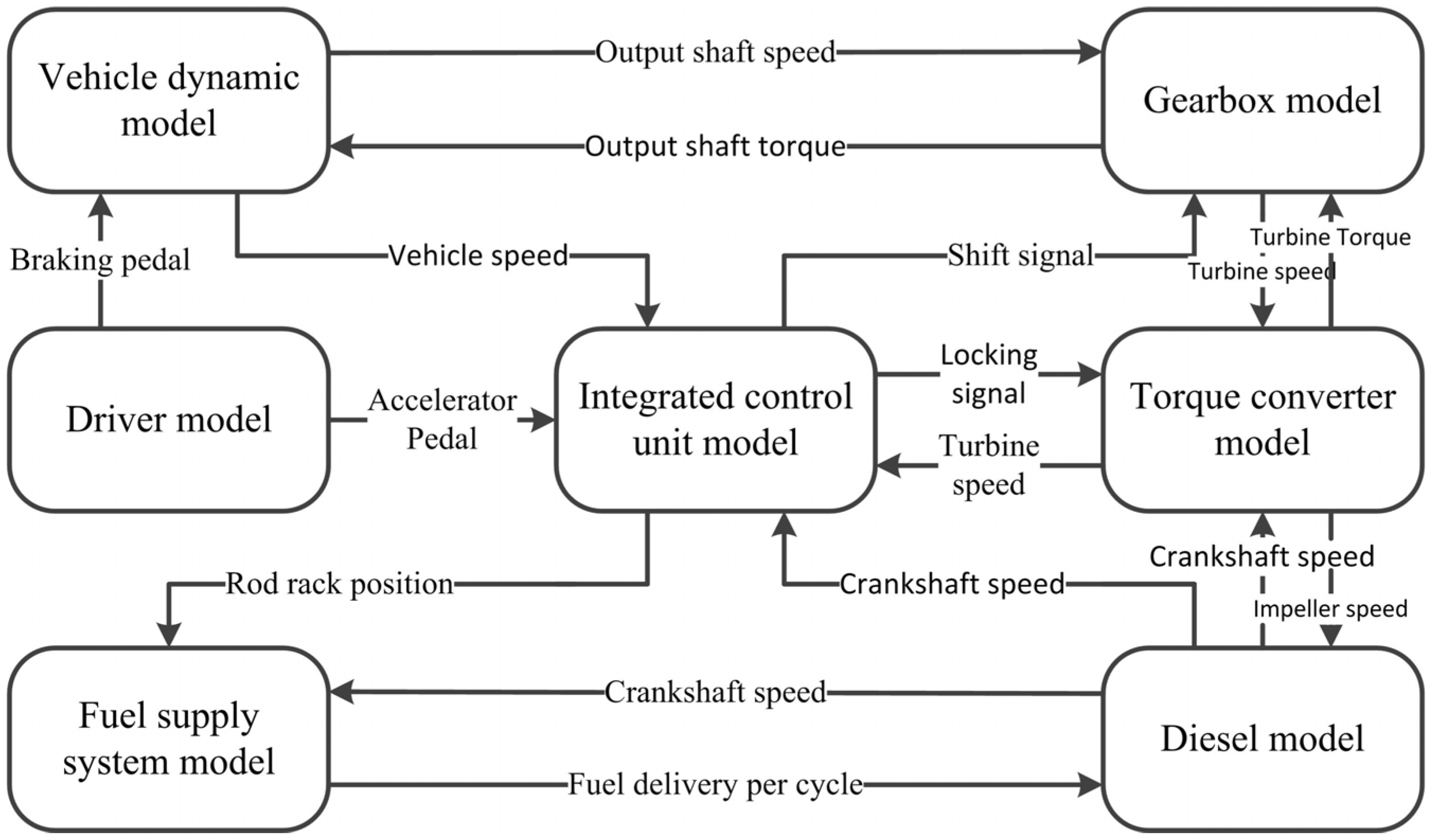
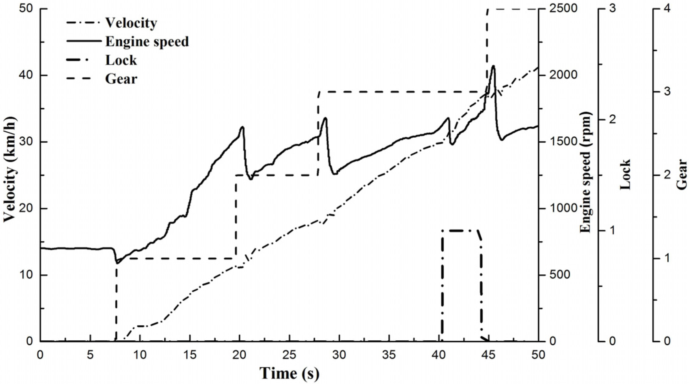
2.2. Real-Time Dynamic Model of Powertrain

The real-time dynamic model of powertrain contains a diesel model, torque converter model, gearbox model, integrated control unit model and vehicle dynamic model. The external parameters which are imported into the driver model are the accelerator pedal position, braking pedal position and vehicle road driving conditions. The structure of the powertrain real-time dynamic model is shown in Figure 3 [16].

Figure 3. Real-time model structure.

Figure 3. Real-time model structure.

2.2.1. Diesel Model

The diesel model contains a compressor model, intercooler model, intake manifold model, exhaust pipe model, turbine model, supercharger rotor dynamic model, fuel supply system model, combustion model and crankshaft dynamic model [17].

2.2.2. Torque Converter Model

The torque converter consists of an impeller, turbine and reactor fastened to the crust. The impeller is connected with the torque converter input shaft, and the turbine is connected with the torque converter output shaft [18]. The torque of impeller shaft and the torque of turbine can be calculated as follows:

$$M_b={\text{λ}}_b\text{γ}{n}_b^2{D}^5$$

(1)

$$M_w={\text{λ}}_w\text{γ}{n}_b^2{D}^5$$

(2)

In the formulas, $M_b$ is the torque of the impeller shaft, $M_w$ is the torque of the turbine, γ is the density of the liquid in the torque converter, $D$ is the effective diameter of the impeller, $n_b$ is the speed of the impeller, ${\text{λ}}_b$ is the torque ratio of the impeller, and ${\text{λ}}_w$ is the torque of the turbine.

2.2.3. Gearbox Model

The gearbox, which is hydraulic-mechanical, contains the input shaft, countershaft, output shaft and four clutches identified as CL, CH, C1 and C2. The relation between gears and clutches is shown in Table 1 [19].

Table 1. Relationship between gears and clutches.

Gear Number	1	2	3	4
CL	√		√
CH		√		√
C1	√	√
C2			√	√

Table 1. Relationship between gears and clutches.

Gear Number	1	2	3	4
CL	√		√
CH		√		√
C1	√	√
C2			√	√

2.2.4. Driver Model

The driver model is established for simulating the real driving cycle of a heavy-duty vehicle. In the model, the real velocity of the current step is used as the input signal and contrasted with the target velocity of the particular driving cycle [20]. By inputting into the PID (Proportion Integration Differentiation) control the difference between the vehicle’s real and target velocity, the accelerator pedal signal and the braking pedal signal are calculated and then converted into voltage signals by way of D/A conversion channel of dSPACE. The signals are delivered to the powertrain integrated control unit to follow the target velocity [21].

By gathering and analyzing the driving parameters of heavy-duty vehicles, the driving cycle is established in statistical theory. This paper applies the method of establishing the driving cycle of heavy-duty vehicles developed by Lu et al. [22]. The form of the driving cycle is a velocity-time curve. What’s more, the building process of the driving cycle, shown in Figure 4, contains five steps: Step 1: the kinematic sample is obtained, which is defined as a complete one circle driving test. Step 2: the characteristic value of each sample is calculated. Step 3: the correlation analysis is conducted to select the representative sample. Step 4: the distribution characteristic value of the sample is calculated for further helping the selection in Step 3. Step 5: the slope information of the driving cycle is added for off-road heavy-duty vehicles. By doing the steps mentioned above, two typical driving cycles are obtained, which can simulate the majority of heavy-duty vehicle driving conditions. Meanwhile, the road surface roughness, the driving cycles and the road grade-distance are also considered. Besides, the road gradient resistance of the vehicle dynamic model reflects the influence on the vehicle. As for results, a smooth driving cycle is shown in Figure 5 and Figure 6. The complex driving cycle is shown in Figure 7 and Figure 8.

Figure 4. The building process of driving cycle.

Figure 4. The building process of driving cycle.

Figure 5. Smooth driving cycle (velocity-time).

Figure 5. Smooth driving cycle (velocity-time).

Figure 6. Smooth driving cycle (road grade-distance).

Figure 6. Smooth driving cycle (road grade-distance).

Figure 7. Complex driving cycle (velocity-time).

Figure 7. Complex driving cycle (velocity-time).

Figure 8. Complex driving cycle (road grade-distance).

Figure 8. Complex driving cycle (road grade-distance).

2.2.5. Vehicle Dynamic Model

The external resistances during heavy-duty vehicle driving are rolling resistance, gradient resistance and air resistance. They are calculated as follows:

$$R_l=fG\cos \alpha$$

(3)

$$R_p=G\sin \alpha$$

(4)

$$R_k=CA{v}^2$$

(5)

In the formulas, R_l denotes the rolling resistance, while f stands for the rolling resistance coefficient, G for the gravity of the vehicle, and α for the road slope angle; R_p for the gradient resistance, R_k for the air resistance, C for the air drag coefficient, A for the vehicle’s positive projection area, and v for the velocity.

While the heavy-duty vehicle is accelerating, the inertia force of the mass is called acceleration resistance. The acceleration resistance is obtained as follows:

$$R_j=\text{δ}m\frac{dv}{dt}$$

(6)

In the formula, R_j represents the acceleration resistance, δ is the mass addition coefficient, m is the mass of the vehicle. Considering the powertrain efficiency, the driving force is as follows:

$$F_q=\frac{T_{e}i{\text{η}}_d{\text{η}}_c}{r}$$

(7)

In this formula, Fq is the driving force, Te is the engine output shaft torque, i is the ratio of the engine output shaft to the wheel, ${\text{η}}_d$ is the coefficient of the power plant, ${\text{η}}_c$ is the coefficient of the transmission, and r is the wheel radius. By Newton’s second law, the vehicle driving force is equated with the resistances, namely:

$$F_q=R_l+R_p+R_k+R_j$$

(8)

3. Results

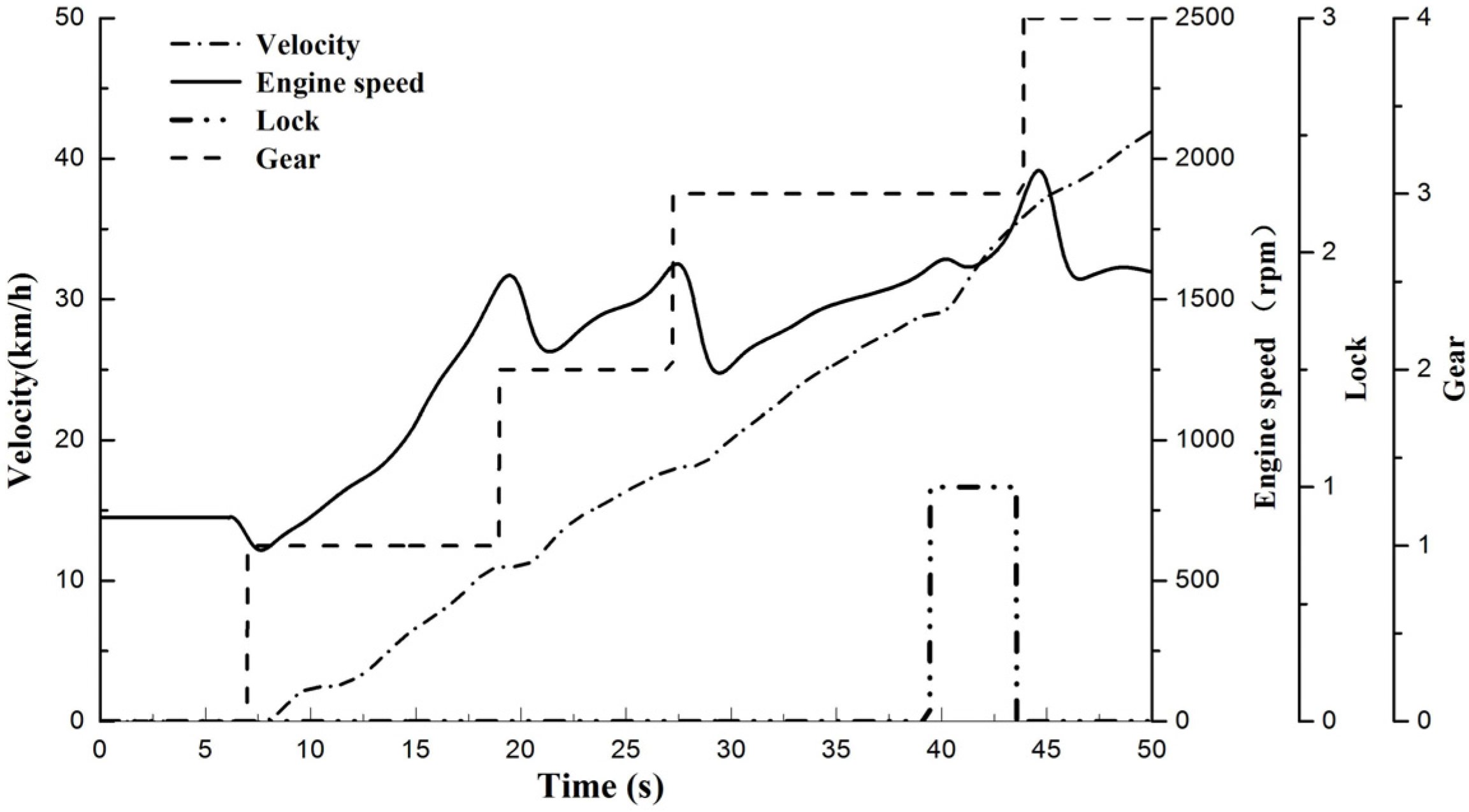
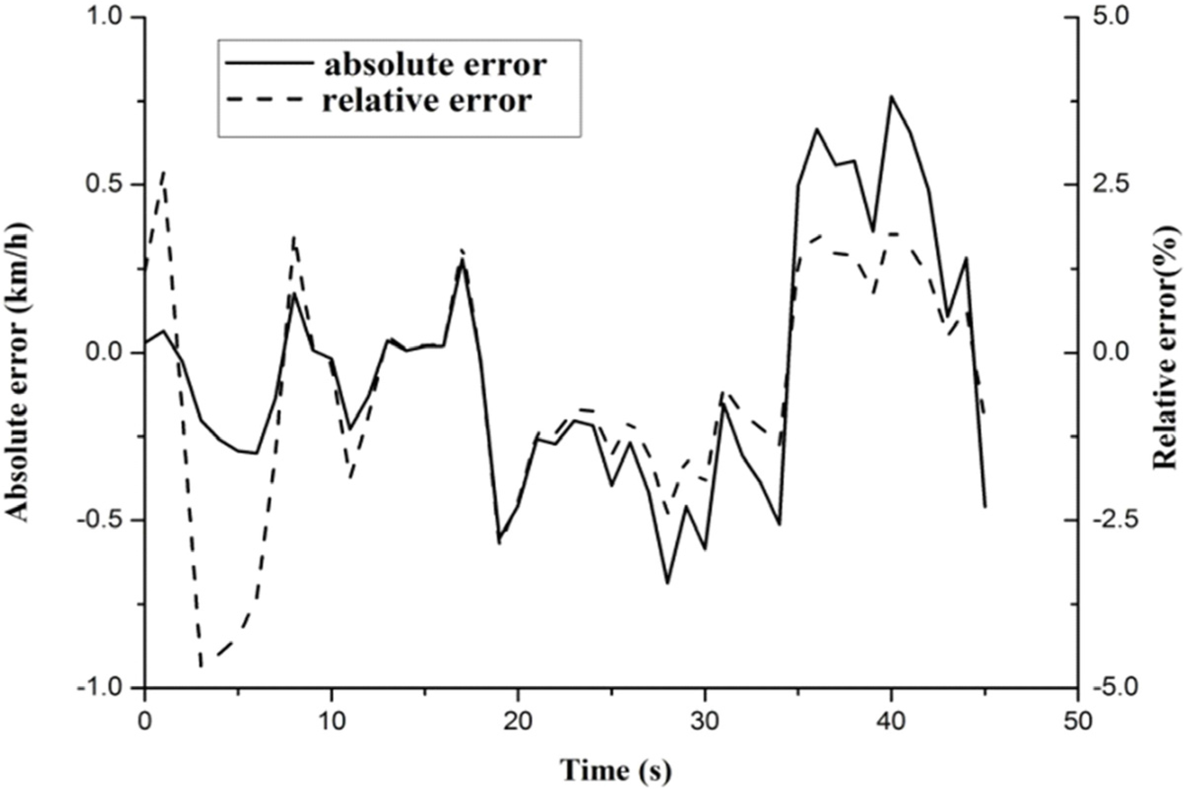
3.1. Certifying the Virtual Calibration Platform

After establishing the virtual calibration platform, the real time performance, the precision and the manageability of the platform should be certified. Then the virtual calibration can replace the bench test and the road test to a certain degree.

Therefore, the results of the virtual calibration in the smooth driving cycle are compared with the real experimental data of some heavy-duty vehicles in an experimental field which corresponds with a smooth driving cycle. The real experimental data is shown in Figure 9. From the figure, the real driving manners of the real vehicle can be obtained. Then the manners are input into the driver model of the virtual calibration platform. The results of the virtual calibration are shown in Figure 10. Figure 11 is the comparison between the simulation velocity and the real velocity.

To compare the data distinctly, this paper selects the previous 50 s of the entire cycle as shown in Figure 9 and Figure 10. From the figures, the trend of the corresponding curves is identical. The times (the shift time, the locking time, the acceleration time, etc.) coincide. The corresponding deviations of the times are less than 5%, so the virtual calibration platform has a good real time performance. From Figure 11, it can be seen that the relative error between the simulation velocity and the real velocity is less than 5% in the whole acceleration process, so the virtual calibration platform has good precision. Therefore, the virtual calibration can simulate the real driving conditions.

Figure 9. Real vehicle experimental data.

Figure 9. Real vehicle experimental data.

Figure 10. Simulation data of the virtual calibration system.

Figure 10. Simulation data of the virtual calibration system.

Figure 11. Error between the simulation velocity and the real velocity.

Figure 11. Error between the simulation velocity and the real velocity.

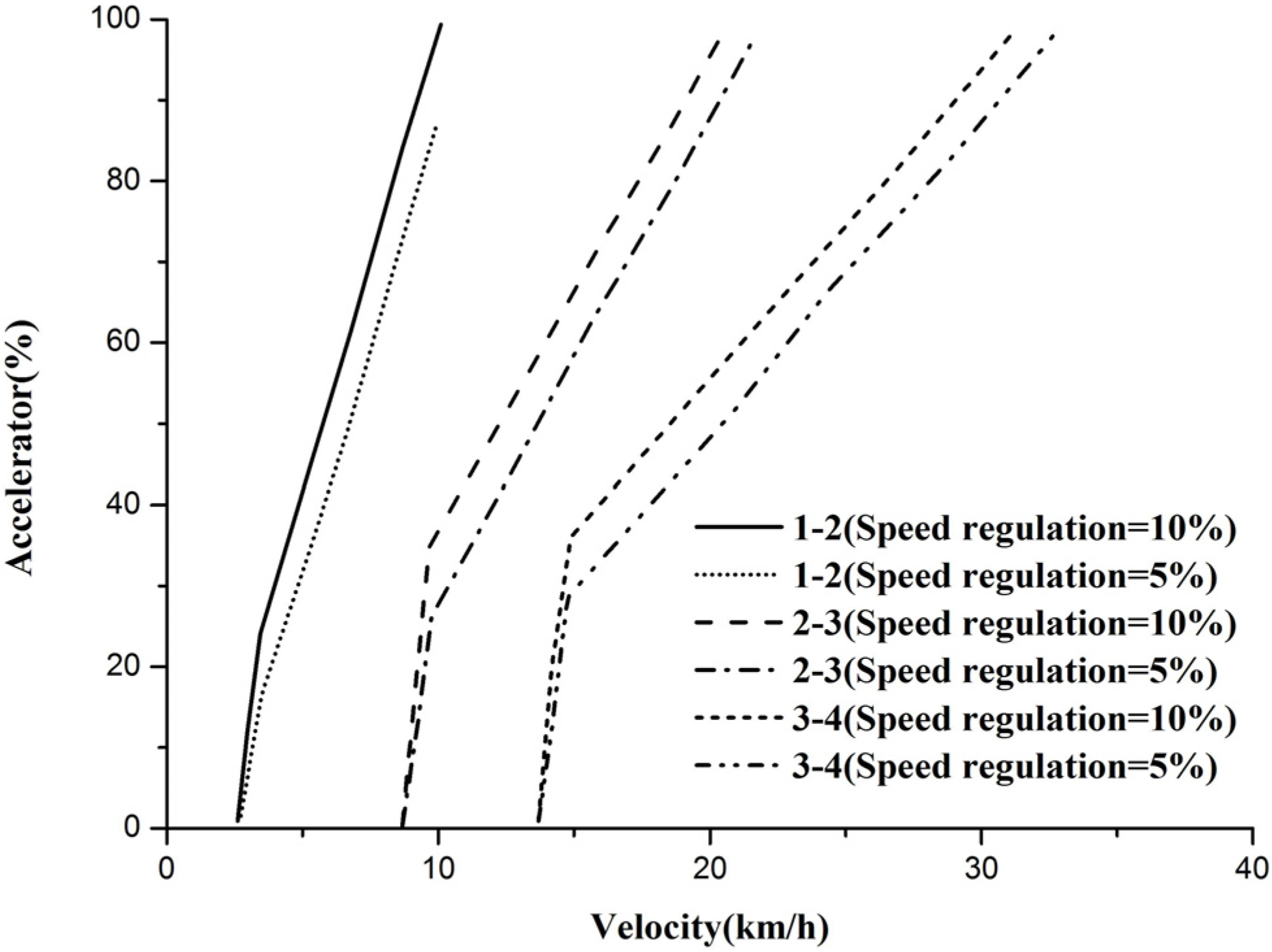
3.2. Economic Shift Schedule

The economic shift schedule is a function of the acceleration and the velocity. The economic shift schedule is made up of four steps: (1) the fuel consumption-speed curve at each gear is obtained while the vehicle is running at a certain acceleration velocity. (2) The intersection points of adjacent fuel consumption curves are set as the shift points (1-2, 2-3, 3-4) at this acceleration velocity. (3) Acceleration and speed at each shift point are obtained. (4) The discrete points at different acceleration velocities are used to draw the acceleration-speed curve and that is one economic shift schedule.

By changing the speed regulation and repeating the above operations, the economic shift schedules of different speed regulations are obtained, as shown in Figure 12.

Figure 12. Economic shift schedules with different speed regulation.

Figure 12. Economic shift schedules with different speed regulation.

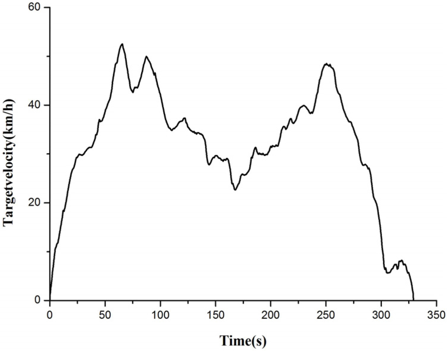
3.3. Virtual Calibration of Economic Shift Schedule Based on Driving Cycles

By applying the smooth driving cycle as shown in Figure 5 and Figure 6 and setting the economic shift schedule of different speed regulations to the integrated control unit of the powertrain, the virtual calibration platform does real-time simulations. The fuel consumptions are obtained from the vehicle’s fuel consumption model in the entire cycle. The fuel consumption percentage in the smooth driving cycle is shown in Figure 13. The fuel consumption percentage is defined as 100% when the vehicle applies the original speed regulation and shift schedule. By applying the complex driving cycle as shown in Figure 7 and Figure 8, and repeating the above operations, the fuel consumption percentage in the complex driving cycle is obtained, as shown in Figure 14.

In Figure 13, the abscissa is the speed regulation and the ordinate is the fuel consumption percentage. When the speed regulation is 6%, the fuel consumption percentage is 100% which is the maximum. As the speed regulation gets bigger, the consumption percentage gets smaller. When the speed regulation is 12%, the fuel consumption percentage is the minimum and reduced by 13%, so in the smooth driving cycle, when the powertrain applies a larger speed regulation and the corresponding shift schedule, the vehicle has better economic performance.

In Figure 14, when the speed regulation is 5%, the fuel consumption percentage is the minimum and reduced by 5%. As the speed regulation gets bigger, the consumption percentage gets larger. When the speed regulation is 12%, the fuel consumption percentage is 99.36% and reduced by 0.64%, which is the maximum, so in the complex driving cycle, when the powertrain applies a smaller speed regulation and the corresponding shift schedule, the vehicle has better economic performance.

Figure 13. Fuel consumption percentage in the smooth driving cycle.

Figure 13. Fuel consumption percentage in the smooth driving cycle.

Figure 14. Fuel consumption percentage in the complex driving cycle.

Figure 14. Fuel consumption percentage in the complex driving cycle.

3.4. Real Vehicle Confirmatory Experiment

In order to certify the results from the virtual calibration platform, the paper describes real road tests which correspond the smooth and complex driving cycle as shown in Figure 4, Figure 5 and Figure 6. The experimental vehicle is same as the one applied in the virtual calibration platform. The experimental fields are prototypes of the smooth and complex driving cycles.

The heavy-duty vehicle applies the original speed regulation and shift schedule and performs the smooth and complex road tests. In the field which corresponds the smooth driving cycle, the fuel consumption percentage of the real vehicle confirmatory experiment in the smooth road is obtained as shown in Figure 15, by setting the speed regulation at 12% and the corresponding shift schedule to the integrated control unit of powertrain. In the field which corresponds the complex driving cycle, the fuel consumption percentage of real vehicle confirmatory experiment in the complex road is obtained as shown in Figure 16, by setting the speed regulation as 5% and the corresponding shift schedule to the integrated control unit of powertrain.

Figure 15. Fuel consumption percentage of real vehicle confirmatory experiment in the smooth driving cycle.

Figure 15. Fuel consumption percentage of real vehicle confirmatory experiment in the smooth driving cycle.

Figure 16. Fuel consumption percentage of real vehicle confirmatory experiment in the complex driving cycle.

Figure 16. Fuel consumption percentage of real vehicle confirmatory experiment in the complex driving cycle.

In Figure 15, when the heavy-duty vehicle applies the regulation on a level of 12% and abides by corresponding shift schedule, the fuel consumption can be reduced be 11.2%. In Figure 16, when the heavy-duty vehicle applies the regulation 5% and abides by the corresponding shift schedule, the fuel consumption is reduced by 5.7%. The results correspond to one of the virtual calibration platforms, thus it proves that the proposed virtual calibration platform is feasible.

4. Conclusions

• Fuel economy improvement for a heavy-duty powertrain was performed on a dSPACE hardware-in-loop simulation and calibration test bench, which is valuable for a more efficient and easier shift schedule calibration for an off-road heavy-duty powertrain.
• For diesel powertrains, especially when an all-speed governor is employed, optimization of the speed governing rate and shift schedule should be conducted. For the first time, by using the s virtual calibration platform, the corresponding work was successfully performed.
• A real road test which corresponds to the smooth and complex driving cycles was performed in order to verify the results of the virtual calibration platform. As the results show, it is reasonable and effective to carry out virtual calibration of economic shift schedules for heavy-duty vehicles. This is proved conclusively to be instructive for calibrating a real heavy-duty vehicle’s economic performance.
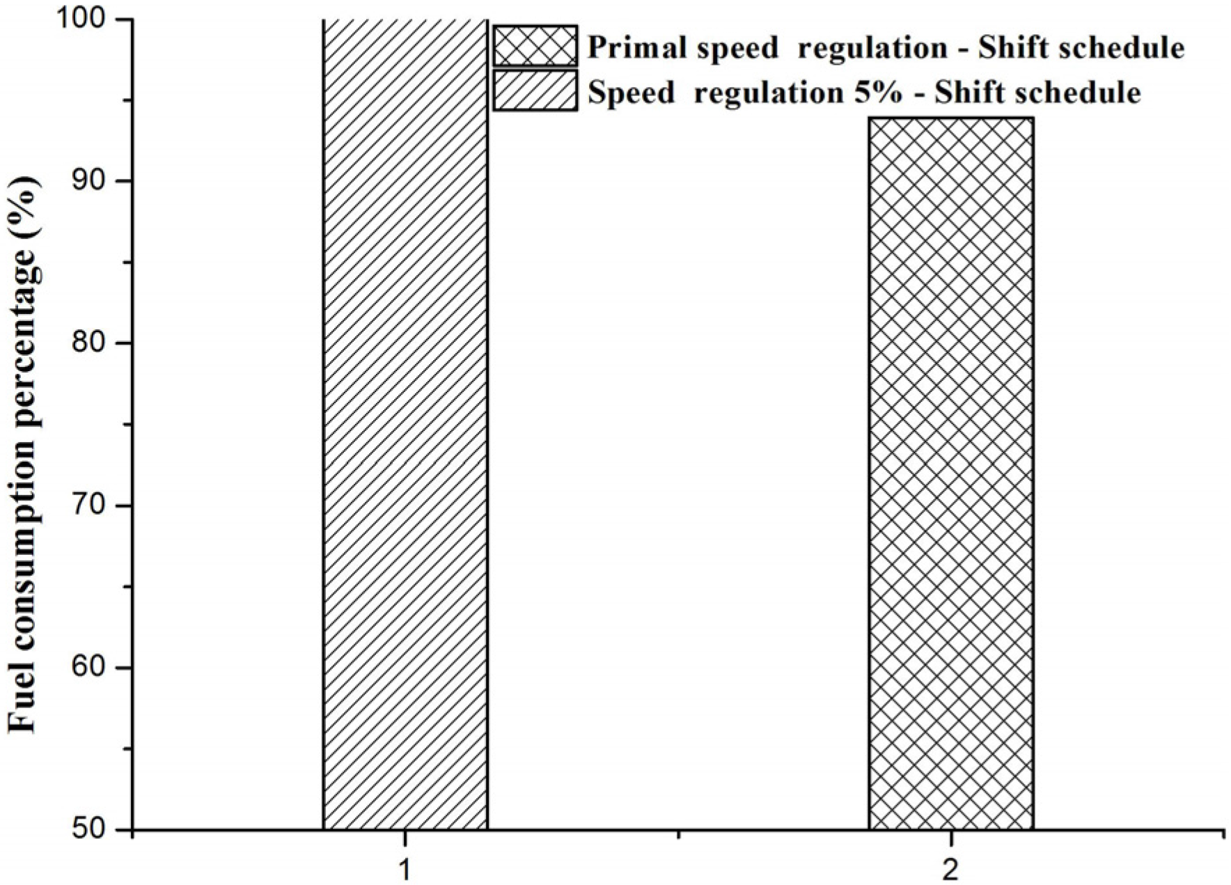
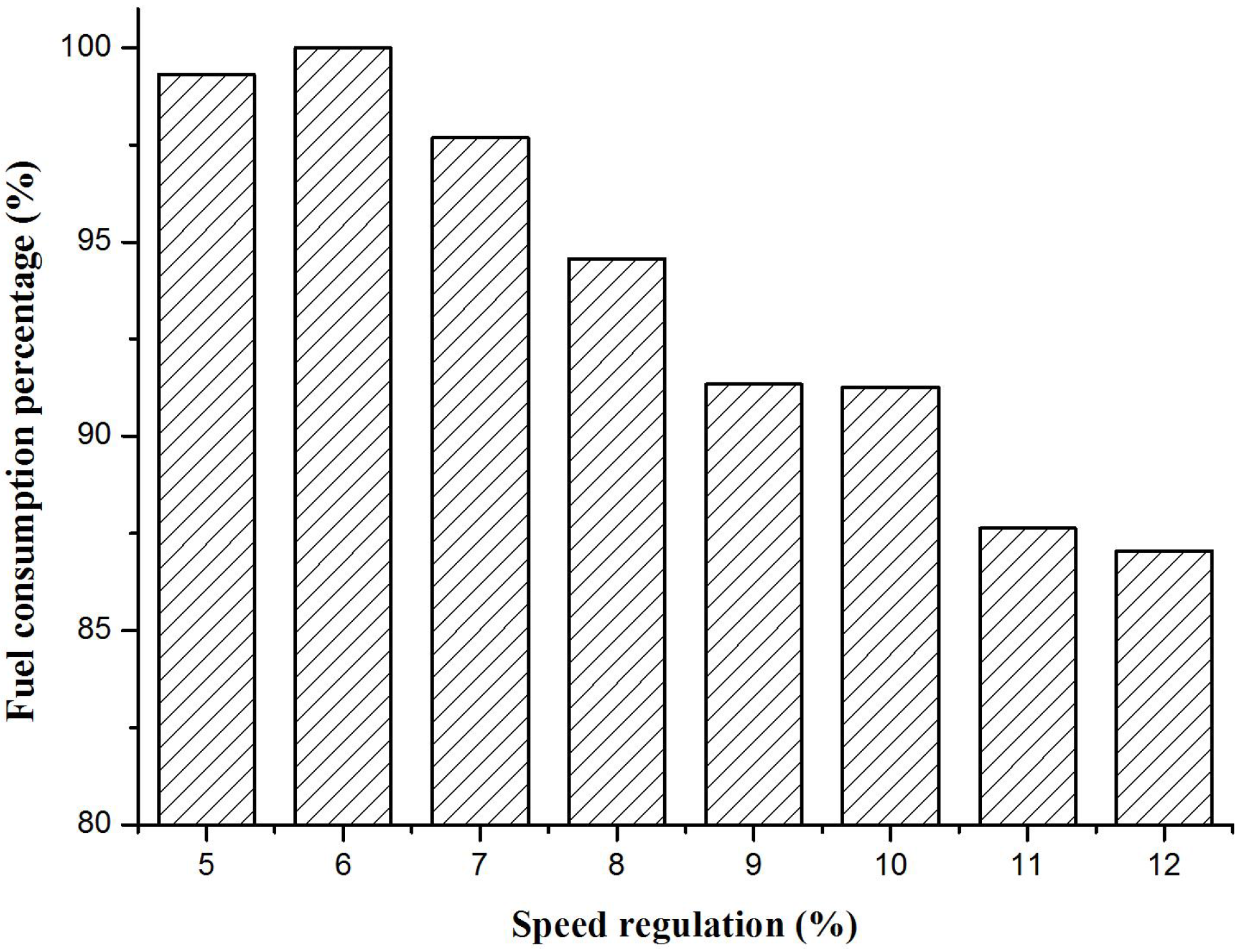
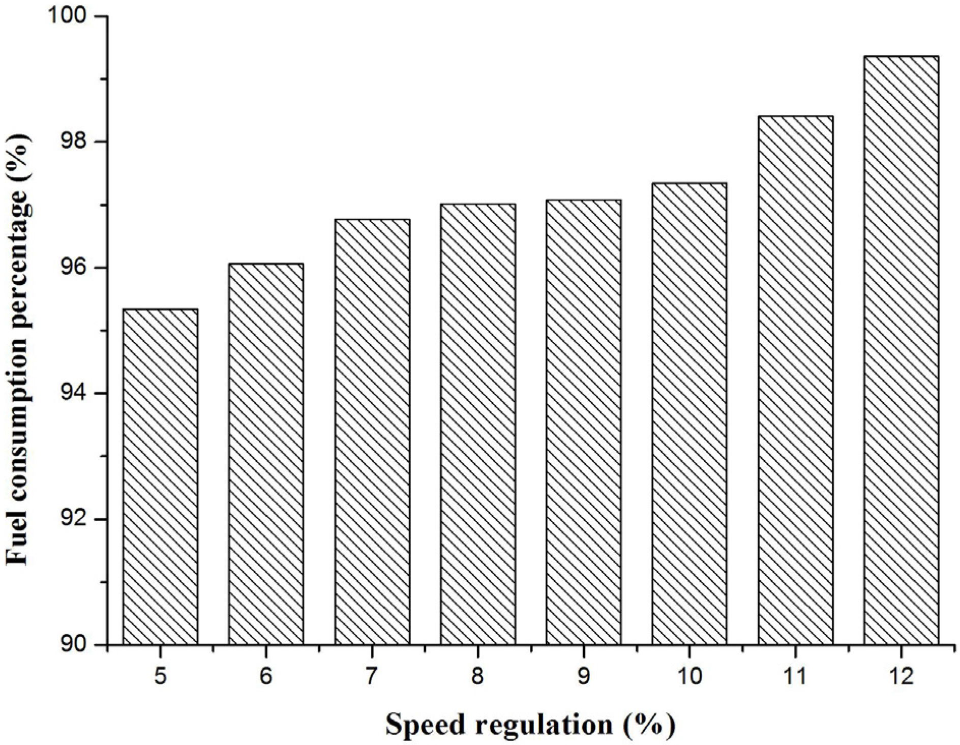
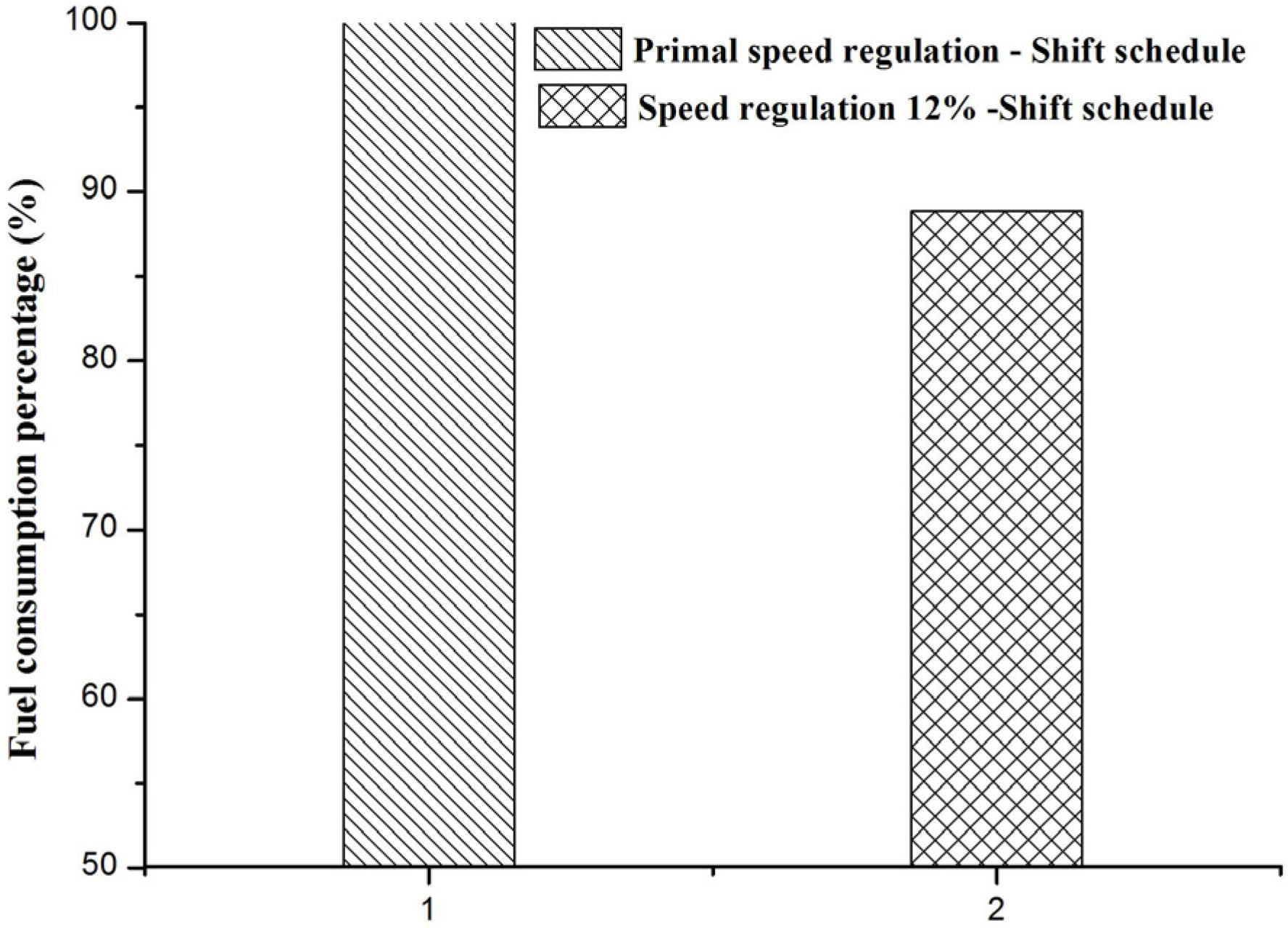
• By virtual calibration, it is shown that in the smooth driving cycle, when the powertrain applies a larger speed regulation such as 12% and the corresponding shift schedule is used, the fuel consumption is smaller and reduced by 13%. In the complex driving cycle, when the powertrain applies a smaller speed regulation such as 5% and the corresponding shift schedule, the fuel consumption is smaller and reduced by 5%. By matching the best regulation of economic shift schedule under different road conditions, the fuel economy of vehicles can be improved.

References

1. Pelkmans, L.; de Keukeleere, D.; Bruneel, H.; Lenaers, G. Influence of Vehicle Test Cycle Characteristics on Fuel Consumption and Emissions of City Buses; SAE Technical Paper No.2001-01-2002; SAE International: Warrendale, PA, USA, 2001. [Google Scholar]
2. Yu, Z.S. Automobile Theory; China Machine Press: Beijing, China, 2009. (In Chinese) [Google Scholar]
3. Bruneel, H. Heavy Duty Testing Cycles Development: A New Methodology; SAE Technical Paper No.2000-01-1860; SAE International: Warrendale, PA, USA, 2000. [Google Scholar]
4. Zhang, F.X. Study on Urban Vehicle Conditions. Master’s Thesis, Wuhan Polytechnics University, Wuhan, China, 2005. [Google Scholar]
5. Zhang, J.W.; Li, M.L.; Ai, G.H.; Zhang, F.X.; Zhu, X.C. Study on vehicle driving cycles and performances. Automot. Eng. 2005, 27, 220–224. [Google Scholar]
6. Song, B.Z. Study on Real Driving Cycles in Xi’an. Master’s Thesis, Traffic Environment and Safety Technology of Changan University, Xi’an, China, 2009. [Google Scholar]
7. Pan, Z.Y. Study on Driving Cycles of Urban Buses. Master’s Thesis, Dalian University of Technology, Dalian, China, 2009. [Google Scholar]
8. Sun, Y.G.; Zhao, C.L.; Liu, B.L.; Zhang, F.J. Active control technology of engine forpowertrain plant during upshifting. Acta Armamentarii 2014, 35, 312–317. (In Chinese) [Google Scholar]
9. Zhang, S.M. An Investigation on Model-Based Virtual Calibration System of Engines with EFI. Master’s Thesis, Tianjin University, Tianjin, China, 2008. [Google Scholar]
10. Chen, L.Y. An Investigation on Model-Based Virtual Calibration System of High Pressure Common Rail Diesel Engine. Master’s Thesis, Tianjin University, Tianjin, China, 2007. [Google Scholar]
11. Catania, A.E.; Finesso, R.; Spessa, E. Predictive zero-dimensional combustion model for DI diesel engine feed-forward control. Energy Convers. Manag. 2011, 52, 3159–3175. [Google Scholar] [CrossRef]
12. Finesso, R.; Spessa, E. A real time zero-dimensional diagnostic model for the calculation of in-cylinder temperatures, HRR and nitrogen oxides in diesel engines. Energy Convers. Manag. 2014, 79, 498–510. [Google Scholar] [CrossRef]
13. d’Ambrosio, S.; Finesso, R.; Fu, L.; Mittica, A.; Spessa, E. A control-oriented real-time semi-empirical model for the prediction of NOx emissions in diesel engines. Appl. Energy 2014, 130, 265–279. [Google Scholar] [CrossRef]
14. Li, C.W.; Zhang, H.B.; Zhao, C.L.; Zhang, F.J.; Huang, Y.; Sun, Y.B. Study on electronic control unit hardwares in the loop simulation platform of engine control systems based on dSPACEsystem. Acta Armamentarii 2004, 25, 402–406. (In Chinese) [Google Scholar]
15. Hanselmann, H. Hardware-in-the-loop Simulation as a Standard Approach for Development, Customization and Production Test; SAE 931953; SAE International: Warrendale, PA, USA, 1993. [Google Scholar]
16. Goldsmith, S. A Practical Guide to Real-Time Systems Development; Prentice-Hall, Inc.: Upper Saddle River, NJ, USA, 1993. [Google Scholar]
17. Isermann, R.; Sinsel, S.; Schaffnit, J. Modeling and Real-Time Simulation of Diesel Engines for Control; SAE 980796; SAE International: Warrendale, PA, USA, 1998. [Google Scholar]
18. Ma, C. Study on Locking Control of Lock-up Torque Converter. Master’s Thesis, Beijing Institute of Technology, Beijing, China, 2004. [Google Scholar]
19. Yan, Q.D.; Zhang, L.D.; Zhao, Y.Q. Structure and Design of Tank (Part II); Beijing Institute of Technology Press: Beijing, China, 2007. (In Chinese) [Google Scholar]
20. Zhou, Y.B.; Yan, Q.D.; Li, H.C. Road roughness research of tracked vehicle compliance simulation experiment. J. Syst. Simul. 2006, 18, 95–97. [Google Scholar]
21. Yuan, H.J.; Zhang, F.J. Simulation about power performance of tracked vehicles and analysis of parameters of the law. Veh. Power Technol. 2010, 1, 20–25. [Google Scholar]
22. Lu, H.Z.; Zhang, F.J.; Zhao, C.L.; Shi, Y.; Yuan, H.J. Investigation on a construction method of driving cycle for tracked vehicle. Acta Armamentarii 2011, 32, 1041–1046. (In Chinese) [Google Scholar]