Economic and Environmental Performances of Small-Scale Rural PV Solar Projects under the Clean Development Mechanism: The Case of Cambodia

Abstract

The two core objectives of the Clean Development Mechanism (CDM) are cost-effective emission reduction and sustainable development. Despite the potential to contribute to both objectives, solar projects play a negligible role under the CDM. In this research, the greenhouse gas mitigation cost is used to evaluate the economic and environmental performances of small-scale rural photovoltaic solar projects. In particular, we compare the use of absolute and relative mitigation costs to evaluate the attractiveness of these projects under the CDM. We encourage the use of relative mitigation costs, implying consideration of baseline costs that render the projects profitable. Results of the mitigation cost analysis are dependent on the baseline chosen. To overcome this drawback, we complement the analysis with a multi-objective optimization approach, which allows quantifying the trade-off between economic and environmental performances of the optimal technologies without requiring a baseline.

1. Introduction

Countries committed to the Kyoto Protocol must meet greenhouse gas (GHG) emission reduction targets primarily through national measures. As an additional means of compliance, the Kyoto Protocol launched three market-based mechanisms, thereby creating the “carbon market”. These mechanisms are (i) Emissions Trading (ET); (ii) Joint Implementation (JI); and (iii) the Clean Development Mechanism (CDM). The ET allows countries that have spare emission units to sell this excess capacity to countries that are over their targets. The JI and CDM are both project-based mechanisms that feed the carbon market. The former enables industrialized countries to carry out joint projects with other developed countries, while the latter involves investment in sustainable development projects that reduce emissions in developing countries [1]. Moreover, in the CDM, projects can earn saleable certified emission reduction (CER) credits—each equivalent to one ton of CO₂—that can be used towards meeting the Kyoto targets [2].

In particular, the CDM is designed to meet two objectives, namely to help Annex I parties (developed countries with specific limitation targets for GHG emissions) to cost-effectively meet part of their reduction targets and to assist non-Annex I parties (developing countries under the Kyoto Protocol without legally binding emission reduction targets) in achieving sustainable development [3]. In literature, it is argued that both objectives are contradictory, with the cost-effective reduction objective overshadowing the sustainable development goal. Amongst others, Sutter and Parreño [4] find a trade-off strongly in favor of the cost-effective emission reduction objective, while neglecting the sustainable development goal. Based on a literature review, Olsen [5] confirms that a trade-off between the CDM’s twin objectives exists and that, when left to market forces, the CDM does not significantly contribute to sustainable development. Moreover, Pearson [6] states that the CDM fails to promote sustainable development, a problem of which the cause is fundamental and stems from the CDM structure in which the search for least-cost carbon credits is the paramount consideration. Hence, he argues that most industrialized countries use the CDM merely to reduce their cost of compliance, searching for projects that deliver large volumes of cheap credits. Over the years, most issued CERs came from hydrofluorocarbons (HFC) and nitrous oxide (N₂O) projects, which are argued to yield the least sustainable development benefits [4,7].

Renewable energy projects on the other hand are less commonly implemented under the CDM, despite their large potential to contribute to sustainability. Especially, solar technologies are underrepresented, claiming on average 0.05% of all the issued CERs. Pearson [6] states that questioning whether the CDM is promoting sustainable development can be framed primarily in terms of whether it is promoting renewables in developing countries. Del Rio [8] encourages the deployment of renewable electricity projects such as solar PV, as—apart from contributing to the GHG emission reduction—they provide substantial local economic, social and environmental sustainability benefits to host countries. Kim et al. [9] find that technologies whose primary benefits are sustainable development (such as solar PV) are more likely to be neglected under the CDM. The scarce amount of CER credits from solar projects mainly results from on-grid solar (96% of all registered solar projects are grid-connected installations). Since the deployment of the CDM, no more than 14 off-grid photovoltaic (PV) solar projects (all small-scale projects) have been registered [10]. On average, these small-scale projects are found to contribute to a slightly higher number of sustainable development benefits than large-scale projects. In particular, they deliver more economic and social benefits than large scale projects [7]. Besides providing local villagers in rural areas with household lighting, the small solar lighting projects can provide lighting for night fishing [11] and street vendors [12], amongst other purposes. Hence, in this research, we focus on small-scale rural PV technologies, which play a negligible role under the CDM.

A possible measure to assess the attractiveness of CDM projects is the mitigation cost, that is the average cost per ton CO₂ reduced (mathematical formulae in Section 2.1). A comprehensive analysis of the mitigation cost implies (i) the assessment of the economic costs of the project and (ii) the assessment of the amount of CO₂ equivalent emissions avoided by the project over its lifetime. Low mitigation cost projects imply low economic costs as well as highly avoided CO₂ emission reductions, which are in turn rewarded with saleable CER units. Hence, projects with low mitigation costs are most attractive for the investors to implement, as they enable low-cost procurement of CER credits [9]. The United Nations Framework Convention on Climate Change (UNFCCC) finds solar photovoltaics to be the most expensive technology deployed in the CDM, with an average mitigation cost of $326 per ton CO₂ equivalents [3]. In this research, we evaluate the mitigation cost of small-scale rural solar PV projects. In particular, we compare “absolute” and “relative” mitigation costs. With absolute mitigation costs, we refer to the mitigation cost defined by the UNFCCC [3], in which the complete omission of baseline costs is assumed. To calculate relative mitigation costs on the other hand, avoided baseline costs are deducted from project costs [13].

The mitigation cost analysis allows ranking technologies or projects in order of decreasing cost of emissions abatement or hence in order of increasing attractiveness for the potential CDM project implementer. We note however that the results of this analysis are always dependent on the baseline or reference technology chosen [14]. To overcome this drawback, we propose to complement the mitigation cost analysis with a multi-objective approach in which economic and environmental objectives are simultaneously optimized. Multi-objective optimization is of particular interest when the objectives to be optimized are conflicting [15]. In this case, plural optimal solutions exist. In this research, we use multi-objective optimization to simultaneously optimize off-grid solar technologies from economic and environmental viewpoints. The project implementer can then choose amongst these optimal solutions, according to personal preferences.

Section 2 demonstrates the methods used, including the absolute versus relative costs of mitigation. In Section 3, we apply these methods to two types of small-scale rural PV projects, i.e., solar light emitting diode (LED) lighting and small solar home systems (SHS). We end the paper with a conclusion and discussion of the findings in Section 4.

2. Methodology

2.1. Mitigation Cost Analysis

2.1.1. Absolute Mitigation Cost

To calculate the absolute mitigation cost, we assume complete omission of avoided baseline costs. This approach is used by the UNFCCC [3], in which the methodology for calculating the mitigation costs of CDM projects is described as follows:

“The mitigation cost is the total cost of the project, including initial outlay of capital, the annual operational expenditure and revenues per CER expected for each project. As shown in Equation (1) below, project mitigation cost is defined as the net present value of a project’s annual operations costs less its non-CDM related revenues (e.g., income from electricity sales for wind projects), plus the capital expenditures, all divided by the amount of GHG emission reductions it expects to achieve over its crediting period.”

(p. 93)

$$MC{\left(absolute\right)}_i=\frac{{{\displaystyle \sum }}_{t=1}^{cp}\frac{\left(O{C}_{i,t}-R_{i,t}\right)}{{\left(1+r\right)}^t}+I_{0,\text{i}}}{{{\displaystyle \sum }}_{t=1}^{cp}{A}_{i,t}}=\frac{{{\displaystyle \sum }}_{t=1}^{cp}\frac{\left(O{C}_{i,t}-R_{i,t}\right)}{{\left(1+r\right)}^t}+I_{0,\text{i}}}{{{\displaystyle \sum }}_{t=1}^{cp}{E}_{b,t}-E_{i,t}}$$

(1)

where: MC(absolute)_i is the absolute mitigation cost of project i (in $/t CO₂eq); t denotes a given year during the project crediting period; cp is the length of its crediting period(s) (up to 10 or 21 years); OC_i,t is the operating cost of project i in year t (in $); R_i,t is the non-CER revenue of project i in year t (in $); I_0,i is the initial investment of project i (in $); A_i,t is the abatement (expected emission reduction) achieved in year t (in t CO₂eq), which is defined as the difference between the baseline emissions (E_b,t) and the project emissions (E_i,t) according to CDM baseline methodologies; r is the discount rate (expressed as a decimal; 1% = 0.01).

We define the discounted operating cost minus the non-CER revenue of the project the numerator in Equation (1) as the operating and maintenance cost (O&M cost). As mentioned before, this definition implies the omission of the baseline costs, i.e., costs related to the baseline technology that are avoided due to implementation of the project. Further, the crediting period rather than the operational lifetime is used for the calculation, also in cases in which the operational lifetime exceeds the crediting period. The project participants may choose between two options for the length of a crediting period: (i) a “fixed” crediting period with no possibility of renewal or extension with a length of maximum 10 years or (ii) a “renewable” crediting period with single crediting periods of maximum seven years which may be renewed two times at most (maximum 21 years). The amount of expected emission reductions is determined as the difference between baseline and project emissions, using prescribed CDM baseline methodologies. Note that the mitigation cost defined as such is calculated from the viewpoint of the project developer.

2.1.2. Relative Mitigation Cost

To calculate the relative mitigation cost, avoided baseline costs are deducted from project costs. This is according to the definition of Lazarus et al. [13], in which the greenhouse gas mitigation cost of technology i is defined as the economic cost per ton carbon dioxide equivalents (CO₂eq) avoided when using technology $i$ to replace the baseline technology $\text{b}$. The mitigation cost is considered from the project developer’s point of view. To calculate this cost, we determine the GHG mitigation potential and the additional economic costs of the project technology $\text{i}$ as compared to the reference or baseline technology $\text{b}$ over the technologies’ lifetime $t$ Equation (2). For purposes of comparison, we apply the terminology used in Equation (1). The differences with the absolute mitigation cost in Equation (1) are indicated in grey.

$$\begin{array}{ll}MC{\left(relative\right)}_i& =\frac{{{\displaystyle \sum }}_{t=1}^n\frac{\left(O{C}_{i,t}-R_{i,t}\right)}{{\left(1+r\right)}^t}+I_{0,\text{i}}-{{\displaystyle \sum }}_{t=1}^n\frac{\left(O{C}_{b,t}-R_{b,t}\right)}{{\left(1+r\right)}^t}+I_{0,\text{b}}}{{{\displaystyle \sum }}_{t=1}^n{A}_t}\\ & =\frac{{{\displaystyle \sum }}_{t=1}^n\frac{\left(O{C}_{i,t}-R_{i,t}\right)}{{\left(1+r\right)}^t}+I_{0,\text{i}}-{{\displaystyle \sum }}_{t=1}^n\frac{\left(O{C}_{b,t}-R_{b,t}\right)}{{\left(1+r\right)}^t}+I_{0,\text{b}}}{{{\displaystyle \sum }}_{t=1}^n{E}_{b,t}-E_{i,t}}\end{array}$$

(2)

where: MC(relative)_i is the relative mitigation cost of project i (in $/t CO₂eq); t denotes a given year during the project lifetime; n is the operational lifetime of the project; i refers to the project implemented; b refers to the replaced baseline technology; OC_t is the operating cost in year t (in $); R_t is the non-CER revenue in year t (in $); I₀ is the initial investment (in $); At is the abatement (expected emission reduction) achieved in year t (in t CO₂eq), which is defined as the difference between the baseline emissions (E_b,t) and the project emissions (E_i,t) determined by means of a life cycle analysis (LCA) model; r is the discount rate (expressed as a decimal; 1% = 0.01).

According to this definition, the avoided baseline costs are deducted from the project’s costs. In this research, the replaced baseline technology is determined according to the applicable CDM methodology for purposes of comparison with the absolute mitigation cost. This implies the existence of a replaced baseline technology. Economic costs are calculated over the technologies’ operational lifetime (rather than over the crediting period) by means of life cycle costing. To calculate the amount of emission abatement, we make use of life cycle analysis (LCA); a method to quantify the environmental impact of a product or service over their full life cycle [16]. When undertaking an LCA, there are a number of methodological choices that need to be made. Choosing either an attributional or a consequential modeling approach may have a great influence on the overall outcomes of the study [17]. Each approach however has its own benefits and drawbacks. It may be argued that a consequential approach may be the more appropriate choice for this study, since this research attempts to support future decision-making. However, a consequential LCA requires detailed data on marginal changes in the technological system as a consequence of a choice for a certain product. In this light, one may wonder, for example, how the PV production technology would be affected by an increasing demand for solar lanterns, or where the crude oil would come from if energy demand were to increase. As many of this required data is either unavailable or very uncertain, the authors have opted to use an attributional LCA model in this study. Hence, we make use of average values for current technologies, as available in the EcoInvent database. To calculate the mitigation cost correctly, both the economic analysis and the environmental life cycle analysis must relate to the same functional unit. Amongst others, this approach has been demonstrated by De Schepper et al. [18].

2.2. Multi-Objective Optimization

Results of the mitigation cost analysis are dependent upon the baseline technology chosen. We propose to overcome this drawback by complementing the analysis with a multi-objective optimization approach. Multi-objective optimization is concerned with the simultaneous optimization of plural objective functions. For a nontrivial multi-objective optimization problem, no single solution exists that optimizes all objectives at the same time. In that case, the objective functions are said to be conflicting and plural optimal solutions exist. These solutions are also referred to as “Pareto optimal” or “efficient” solutions. A feasible solution $\widehat{\text{x}}\in \text{X}$ is called efficient or Pareto optimal if there is no other $\text{x}\in \text{X}$ that performs better with respect to all objectives and strictly better on at least one objective. The set of all efficient solutions is called the efficient set. We use the following mathematical formulation [15,19]:

$$\begin{array}{c}\text{Min} z_k\left(x\right) k=1,\dots ,p p\text{ objective functions}\hfill \\ \text{subject to} g_j\left(x\right)\left\{\begin{array}{c}\le \\ =\end{array}\right\}0\hspace{0.17em}\hspace{0.17em}\hspace{0.17em}\hspace{0.17em}j=1,\dots ,m m\text{ constraints}\hfill \\ x_i\in {ℝ}^n\hspace{0.17em}\hspace{0.17em}\hspace{0.17em}\hspace{0.17em}\hspace{0.17em}\hspace{0.17em}\hspace{0.17em}i=1,\dots ,n n\text{ variables}\end{array}$$

In our research, we want to determine the optimal combinations of technologies to provide a certain demand, while simultaneously minimizing economic costs and environmental emissions. To formulate a mathematical model that represents the optimization of the combined use of different technologies of the same type from economic and environmental viewpoint, we refer to De Schepper, et al. [20]. The decision variables, i.e., the amount of technology $\text{i}$ used in the combination of technologies, are denoted by $x_i$. The model contains two objectives: (i) minimizing economic costs and (ii) minimizing environmental emissions. As regards the economic objective function, we distinguish between (i) minimizing lifecycle costs, as is the case for any rational investor and (ii) minimizing solely the cost of investment, as the latter may constitute a huge implementation barrier for poor households. The economic lifecycle (investment) costs and environmental emissions implied by one unit of technology i are represented respectively by the data $c_i^1\left(c_i^{1\prime }\right)$ and $c_i^2$. Furthermore, a required demand d has to be satisfied. In this constraint, qi is defined as the amount of output provided by one unit of technology i. We note that the demand d in our multi-objective optimization problem must correspond to the functional unit of the mitigation cost analysis in order to establish the link between the mitigation cost analysis and the multi-objective optimization approach. Hence, assuming linear relations, the optimization of the use of technologies i to satisfy required demand d can be formulated as a multi-objective linear programming problem (MOLP), which can be solved using a multi-objective simplex method. The MOLP is defined as follows:

$$\begin{array}{c}\text{Min} {\displaystyle \sum }_{i=1}^n{c}_i^1{x}_i\hspace{1em}\hspace{1em}\hspace{1em}\hspace{1em}\hspace{1em}\hspace{1em}\hspace{1em}\hspace{1em}\text{ Economic objective function}\hfill \\ \text{Min} {\displaystyle \sum }_{i=1}^n{c}_i^2{x}_i \hspace{1em}\hspace{1em}\hspace{1em}\hspace{1em}\hspace{1em}\text{ Economic objective function}\hfill \\ \text{Subject to} {\displaystyle \sum }_{i=1}^n{q}_i{x}_i=d \hspace{0.17em}\hspace{0.17em}\text{ Demand constraint}\end{array}$$

3. Case: Small-Scale Rural Solar PV Projects under the CDM

In our research, we focus on two types of small-scale rural solar PV projects with lighting purposes, which play a negligible role under the CDM in spite of their large sustainability potential. More specifically, we consider small-scale portable solar LED lanterns and small off-grid solar home systems (SHS). In particular, we consider a case in Cambodia, where the electrification rate is merely 24% [21] and the market for modern off-grid lighting is nascent [22]. The Kamworks company is one of the few that provides off-grid lighting to local villagers. They produce and distribute portable solar lanterns—a.k.a. “The Moonlight”—as well as the SHS. In practice, the SHS produce more electricity than is needed for lighting purposes only. Nonetheless, to compare the SHS with the other lighting systems in our analysis, we assume that all available energy is used for lighting. This approach is, amongst others, also used in [23]. The case is hypothetical and did not apply for registration under the CDM. For each type of technology, we discuss (i) The projects and methodologies approved under the CDM; (ii) A brief description, including economic and technical data; and (iii) The calculation of the absolute and relative greenhouse gas mitigation cost, including a sensitivity analysis of the results. As functional unit of our GHG mitigation cost calculation, we consider the provision of light of 100,000 households with typical lighting needs in Cambodia, i.e., the provision of household lighting with a strength of 90 lumens for 3.5 h a day, 365 days per year, during a period of 10 years (the lifetime of the project technologies). Hence, our functional unit totals 114,975 million lumen-hours over a 10-year time span. As a result, the project and baseline technologies have the same size.

3.1. Mitigation Cost Analysis: Portable Solar LED Lanterns

3.1.1. Approved CDM Projects and Methodologies

Note that in this research, we focus on solar LED lanterns rather than on solar CFL lanterns. This is due to the fact that LED based lanterns are about 20% less expensive than CFL lanterns, and they are hence slowly replacing CFL in solar lighting systems [24]. For portable solar LED systems, two CDM methods are applicable. In January 2003, the Approved Methodology for Small-scale CDM project activities (AMS) I.A “Electricity generation by the user” [25] was launched, applicable to renewable electricity generation such as solar, hydro, wind, or biomass gasification implemented to replace fossil-fuel-fired generation. In November 2010, a specific standardized baseline method AMS-III.AR for “Substituting fuel based lighting with LED/CFL lighting systems” was introduced [26]. To date, no more than 12 solar LED lantern projects have been registered. An overview of the registered solar LED lighting projects sorted by date including the estimated emission reductions in metric tonnes of CO₂eq per annum can be found at the UNFCCC website [10]. We note that, since its introduction, eight out of nine solar LED lighting projects were approved under AMS-III.AR. Accordingly, in this research, we apply the approved baseline AMS-III.AR to determine the solar LED lantern’s absolute mitigation cost. We note that the solar lanterns under consideration fulfill the criteria required by this methodology, i.e., the project activity replaces portable fossil fuel based lamps with LED based lighting systems in residential applications, the project lamps are charged with a photovoltaic system and have a minimum lifetime of 10,000 h with a warranty of more than one year, no more than five lamps per household—three to be precise—are distributed, and measures are limited to emission reductions of less than 60 kt CO₂ equivalents annually. Note that this methodology assumes kerosene lanterns as a standardized baseline technology to be replaced by solar lanterns.

3.1.2. Case Description

Portable solar LED lanterns are considered an alternative for kerosene lanterns in developing countries. An estimated 1.06 million households in Cambodia use kerosene as their primary source for lighting. These are primarily poorer households [22]. Hence, in this research, we consider kerosene lanterns as the baseline technology to be replaced by solar LED lanterns, which is in correspondence with AMS-III.AR of the CDM. Economic and technical data regarding the lanterns is presented in Appendix A. The total light output of one solar lantern with a lighting strength of 30 lumens that is used 3.5 h/day, 365 days/y, over a lifetime of 10 years equals 383,250 lumen-hours. Hence, to provide the total of 114,975 million lumen-hours, 300,000 project solar lanterns are distributed to 100,000 households.

3.1.3. Greenhouse Gas Mitigation Costs

3.1.3.1. Absolute Greenhouse Gas Mitigation Cost

We start by calculating the absolute GHG mitigation cost of solar LED lanterns as defined in Equation (1) (Section 2.1.1). Additionally, as higher purchase prices constitute a huge barrier for implementation, we calculate the absolute mitigation cost when considering merely the cost of investment rather than the full life cycle costs. Economic parameter values (operating costs OC_t, initial investment costs I₀, crediting period cp, and discount rate r) can be found in Appendix A. Note that there are no operational revenues R_t from electricity generation, as the project lamps are not grid-connected. Reduced emissions are calculated as the difference between baseline and project emissions according to AMS-III.AR [26]. The expected emission reduction A_t is detailed in Equation (3), which is adapted from Paragraph 24 in AMS-III.AR (note that references to “Paragraph x” in the remainder of this section always refers to paragraphs in AMS-III.AR). In this equation, N_i stands for the number of solar lanterns distributed and OF_t,i represents the percentage of project lamps distributed to end users that are still operating and in service in the year t. The latter is fixed to 100% for years one, two, and three. For project lamps that claim emission reductions for up to seven years, ex-post monitoring surveys must be conducted to determine the percentage of project lamps that are still operating and in service in years four, five, six, and seven. We assume in our analysis that this number equals to 100% throughout the whole lifetime of the product. We note though that assuming that all lamps are operational up to year seven represents an overestimation of the actual number of lamps in service. Baseline emissions, i.e., avoided emissions from the equivalent baseline lighting system, are calculated according to Paragraph 18, which provides a default emissions factor of 0.092 t CO₂eq per project lamp, assuming a utilization rate of 3.5 h/day, 365 days/y, and a fuel use rate of 0.03 L/h for kerosene lanterns. Project emissions of solar lanterns are nonexistent (Paragraph 21). Results are presented in Table 1(A). Additionally, we have calculated the absolute mitigation cost of solar LED lanterns over a hypothetical crediting period of 10 years. These results will be used in the multi-objective optimization analysis (Section 3.3).

$$A_t=N_i·\left(Baseline emissio{n}_{t,i}-Project emissio{n}_{t,i}\right)*\left(O{F}_{t,i}\right)$$

(3)

Table 1. Greenhouse Gas (GHG) mitigation costs of solar light emitting diode (LED) lanterns vs. kerosene lanterns.

Mitigation costs and emissions	Absolute (7 y)	Absolute (10 y)	Relative (10 y)	Relative (7 y)
(A) Mitigation Cost Analysis
(1) Project inv cost ($): $I_{0,i}$	4,500,000.00	4,500,000.00	4,500,000.00	4,500,000.00
(2) Project O&M cost ($): ${\displaystyle \sum }_t\frac{\left(O{C}_{i,t}-R_{i,t}\right)}{{\left(1+r\right)}^t}$	3,706,261.92	4,760,142.02	4,760,142.02	3,706,261.92
(3) Baseline inv cost($): $I_{0,\text{b}}$	not applicable	not applicable	584,279.92	485,917.78
(4) Baseline O&M cost ($): ${\displaystyle \sum }_t\frac{\left(\text{O}{C}_{b,t}-R_{b,t}\right)}{{\left(1+r\right)}^t}$	not applicable	not applicable	46,411,356.74	34,344,357.03
(1) + (2) − (3) − (4) Additional project cost ($)	8,206,261.92	9,260,142.02	−37,735,494.64	−26,624,012.89
(5) Project emission (t CO2eq)	0.00	0.00	1,602.00	1,518.00
(6) Baseline emission (t CO2eq)	193,158.00	275,940.00	283,605.00	198,523.50
(6) − (5) Emission reduction: ${\displaystyle \mathbf{\sum }}_{\mathit{t}}{\mathit{A}}_{\mathit{t}}$ (t CO2eq)	193,158.00	275,940.00	282,003.00	197,005.50
[(1) + (2) − (3) − (4)]/[(6) − (5)] GHG MC LCC ($/t CO2eq)	42.48	33.56	−133.81	−135.14
[(1) − (3)]/[(6) − (5)] GHG MC I0 ($/t CO2eq)	23.30	16.31	13.89	20.38
(B) Monte Carlo Sensitivity Analysis on GHG MC LCC
Range($/t CO2eq)	[35.49; 50.87]	[27.98; 40.24]	[−186.04; −93.68]	[−190.07; −92.38]
Sensitivity with respect to	Kerosene emission (−67.7%)	Kerosene emission (−67.7%)	Fuel use rate (−34.8%)	Fuel use rate (−34.8%)
	I0 solar lantern (+19.0%)	I0 solar lantern (+16.7%)	Cost of kerosene (−34.8%)	Cost of kerosene (−34.8%)
	Battery cost (+12.8%)	Battery cost (+14.8%)	Kerosene emissions (+23.4%)	Kerosene emissions (+21.3%)

Table 1. Greenhouse Gas (GHG) mitigation costs of solar light emitting diode (LED) lanterns vs. kerosene lanterns.

Mitigation costs and emissions	Absolute (7 y)	Absolute (10 y)	Relative (10 y)	Relative (7 y)
(A) Mitigation Cost Analysis
(1) Project inv cost ($): $I_{0,i}$	4,500,000.00	4,500,000.00	4,500,000.00	4,500,000.00
(2) Project O&M cost ($): ${\displaystyle \sum }_t\frac{\left(O{C}_{i,t}-R_{i,t}\right)}{{\left(1+r\right)}^t}$	3,706,261.92	4,760,142.02	4,760,142.02	3,706,261.92
(3) Baseline inv cost($): $I_{0,\text{b}}$	not applicable	not applicable	584,279.92	485,917.78
(4) Baseline O&M cost ($): ${\displaystyle \sum }_t\frac{\left(\text{O}{C}_{b,t}-R_{b,t}\right)}{{\left(1+r\right)}^t}$	not applicable	not applicable	46,411,356.74	34,344,357.03
(1) + (2) − (3) − (4) Additional project cost ($)	8,206,261.92	9,260,142.02	−37,735,494.64	−26,624,012.89
(5) Project emission (t CO2eq)	0.00	0.00	1,602.00	1,518.00
(6) Baseline emission (t CO2eq)	193,158.00	275,940.00	283,605.00	198,523.50
(6) − (5) Emission reduction: ${\displaystyle \mathbf{\sum }}_{\mathit{t}}{\mathit{A}}_{\mathit{t}}$ (t CO2eq)	193,158.00	275,940.00	282,003.00	197,005.50
[(1) + (2) − (3) − (4)]/[(6) − (5)] GHG MC LCC ($/t CO2eq)	42.48	33.56	−133.81	−135.14
[(1) − (3)]/[(6) − (5)] GHG MC I0 ($/t CO2eq)	23.30	16.31	13.89	20.38
(B) Monte Carlo Sensitivity Analysis on GHG MC LCC
Range($/t CO2eq)	[35.49; 50.87]	[27.98; 40.24]	[−186.04; −93.68]	[−190.07; −92.38]
Sensitivity with respect to	Kerosene emission (−67.7%)	Kerosene emission (−67.7%)	Fuel use rate (−34.8%)	Fuel use rate (−34.8%)
	I0 solar lantern (+19.0%)	I0 solar lantern (+16.7%)	Cost of kerosene (−34.8%)	Cost of kerosene (−34.8%)
	Battery cost (+12.8%)	Battery cost (+14.8%)	Kerosene emissions (+23.4%)	Kerosene emissions (+21.3%)

3.1.3.2. Relative Greenhouse Gas Mitigation Cost

In this section, we calculate the relative GHG mitigation cost of portable solar LED lanterns according to Equation (2) (Section 2.1.2). The project costs are calculated identically to those in Equation (1), with the only exception being the lifetime, which is assumed to be 10 years (Appendix A). Additionally, this calculation requires determination of the baseline costs, i.e., the avoided costs of using kerosene lanterns that would have provided the equivalent amount of lighting. Economic parameter values of kerosene lanterns are provided in Appendix A. Emission reductions A_t are calculated as the difference between baseline and project emissions by means of life cycle analysis. To this end, we updated the model described by Durlinger in [23] and [27], which is an attributional LCA model. Ecoinvent v2.2 data was used to model the background data [28]. The impact assessment method ReCiPe [29] was used to generate characterized results. More precisely, this study applies the result of the mid-point impact category “Climate Change”. The software SimaPro 7.2.2 (PRé consultants, Amersfoort, The Netherlands) was used to model the LCA and to generate results. The life cycle inventory as modeled in SimaPro^® is listed in Appendix A. For purposes of comparison, we also calculate the mitigation cost according to Equation (2) over a lifetime of seven years, which is the maximum crediting period prescribed under AMS-III.AR (n = cp = 7). Results are listed in the last two columns of Table 1. Project costs of the solar lanterns under both methods (absolute and relative) are now equal.

To verify the sensitivity on the deterministic values used in this approach, a Monte Carlo sensitivity analysis is conducted on the GHG mitigation cost considering lifecycle costs, assuming 500,000 trial runs. For each input parameter value, a triangular distribution is assumed with minimum and maximum deviations of −10% and +10% with respect to the assumed values. Results are presented in Table 1(B). We indicate the range of GHG mitigation cost values and the sensitivity information as the percent of the mitigation cost variance due to the spread in the three most influencing parameters. Note that a negative (positive) sign indicates that the GHG mitigation cost will decrease (increase) with an increase of this parameter.

3.1.3.3. Results

From our analysis in which we compared absolute and relative GHG mitigation costs of solar LED lanterns, we conclude the following: It is a major difference whether or not baseline costs are included. The absolute mitigation cost assumes the complete omission of baseline costs, even though the avoided costs of kerosene lanterns are approximately five times higher than those of solar lanterns to provide the equivalent amount of lighting. Moreover, sensitivity analysis of the relative mitigation cost indicates that the baseline costs are the most important parameters to determine the mitigation cost. This provides a clear motivation for using relative rather than absolute mitigation costs to assess the attractiveness of projects. Nonetheless, the UNFCCC defined and applies the absolute mitigation cost for this purpose. They recognize, however, that baseline costs can be significant for many projects, and that the avoided costs of fossil-fired generation render renewable energy projects viable despite their high mitigation costs [3]. Indeed, in our analysis of the solar LED lighting, absolute mitigation costs are found positive while relative mitigation costs are negative. The sensitivity analysis indicates that these signs are maintained despite maximal variations in the parameter values between +10% and −10%. Note that a negative sign in this case means that replacing kerosene with solar LED lanterns provides net benefits to society, with the financial benefits outweighing the costs even before considering the value of reduced emissions. A second difference is the use of a limited crediting period under AMS-III.AR. Moreover, AMS-III.AR restricts the crediting period to a maximum of seven years, while Kamworks assures a solar LED technology operational lifetime of 10 years. Avoided kerosene (baseline) emission is relevant, particularly in determining the absolute mitigation cost. This points to the importance of providing a good estimate of kerosene emissions under AMS-III.AR. Kerosene emissions according to AMS-III.AR (193,158 t CO₂eq) deviate no more than 2% from the emissions assessed using our LCA model (197,006 t CO₂eq), assuming equal utilization, fuel use rates, and lifetimes. We note though that in reality, results can differ due to other fuel consumption rates or use patterns. Furthermore, as our LCA indicates that project emissions (1518 t CO₂eq) represent less than 1% of avoided baseline emissions (198,524 t CO₂eq), it seems reasonable to assume that they are negligible, as is the case in AMS-III.AR. Finally, we note that the purchase price of the solar lanterns (+16.7%) and the batteries (+14.8%)—which constitutes a huge barrier for widespread implementation- indeed has an important impact on the mitigation cost. Nonetheless, the sensitivity analysis indicates that the avoided kerosene emissions have the greatest impact on the mitigation cost (−67.7%).

3.2. Mitigation Cost Analysis: Small-Scale Rural Solar Home Systems

3.2.1. Approved CDM Projects and Methodologies

Under the CDM, small-scale rural solar home systems (SHS) can be registered under two methodologies. One option is to register under AMS-I.A “Electricity generation by the user”, which is in place since January 2003 [25]. Another option is to register under AMS-I.L “Electrification of rural communities using renewable energy”, which was introduced in March 2012 [30]. At this moment, only two small-scale rural SHS projects have been registered, both under AMS-I.A. Accordingly, we apply this method to determine the SHS absolute mitigation cost. With a capacity of 40 Wp per system (Appendix A) or 343kWp in total, this project falls largely under the CDM limit of 15 MW for small-scale systems. We note that AMS-I.A does not specify a baseline for solar home systems. Indeed, in their project design documents, we find that the two registered SHS projects use different baselines. Moreover, “Photovoltaic kits to light up rural households in Morocco” [31] assumes diesel generators for baseline calculations, while “Installation of solar home systems in Bangladesh” [32] assumes the usage of kerosene and batteries charged at shops from small diesel generators as baseline technologies.

3.2.2. Case Description

In Cambodia, the key off-grid lighting sources are kerosene and batteries powered by diesel generators at local shops [22]. Hence, these technologies are considered as baseline for solar home systems. Assuming a lifetime of 10 years, electricity production of 117 Wh/day and a luminous efficacy of 50 Lm/W (data in Appendix A), each SHS provides 21,352,500 lumen-hours. Thus, 5384 SHS are needed to provide the total functional unit of 114,975 million lumen-hours. To provide the equivalent amount of lighting, 22,532 batteries charged with diesel generators or 1,000,000 kerosene lanterns are required.

3.2.3. Greenhouse Gas Mitigation Costs

3.2.3.1. Absolute Greenhouse Gas Mitigation Cost

We start with calculating the absolute GHG mitigation cost of solar home systems according to Equation (1) (Section 2.1.1). Additionally, we calculate the absolute mitigation cost when considering merely the cost of investment rather than the full life cycle costs. Economic parameter values of the SHS are presented in Appendix A. As the systems are not grid-connected, there are no operational revenues (R_t = 0). The expected emission abatement A_t is calculated as the difference of baseline and project emissions minus potential leakage over the crediting period according to AMS-I.A [25]. The energy baseline is the fuel consumption that would have been used in the absence of the project activity to provide the equivalent quantity of lighting. We compare the choice of (i) kerosene and (ii) batteries powered at diesel stations as baselines.

The kerosene baseline is calculated according to option 3 of AMS-I.A (Paragraph 8). In the remainder of this section, all “Paragraph” references refer to the paragraphs in AMS-I.A. In correspondence with Paragraph 10, the baseline emissions in year t (E_b,t) due to the replacement of kerosene consumption is calculated in Equation (4), with N_t the number of kerosene lamps replaced in year t (1,000,000 lamps with a lifetime of two years over a period of 10 years or hence 200,000 lamps each year), FC_t the amount of kerosene consumption per lamp in year t (0.03 L/h × 3.5 h/day × 365 days/y × 0.8026 kg/L = 30.76 kg/y), NCV the net caloric value of kerosene (43.8 TJ/Gg [33]) , and EFCO₂ the CO₂ emission factor of kerosene (71.9 kgCO₂/GJ [33]). This leads to an annual emission of 0.097 t CO₂eq/kerosene lamp. We note that this differs from the default value described under AMS-III.AR (0.092 t CO₂eq/project lamp), although it relates to the exact same baseline technology. Baseline emissions of kerosene lanterns in year t equal 19,374 t CO₂eq. There are no project emissions (Paragraph 13). Leakage is assumed to be zero. Results are shown in the first column of Table 2(A).

$$E_{b,t}=N_t·F{C}_t·NCV·E{F}_{CO2}$$

(4)

When considering batteries powered at diesel stations as baseline, emissions (E_b,t) are calculated according to option 2 of AMS-I.A (Paragraph 8) in Equation (5) as the sum of the annual output of all i renewable energy technologies implemented as part of the project activity (${\displaystyle \sum }_{\text{i}}E{G}_i)$, considering average annual distribution losses ($l$) that would have been observed in diesel-powered mini-grids. Each SHS produces 117 Wh/day (Appendix A) and no distribution losses are considered ($l=0)$. Given a total of 5384 SHS, the energy baseline thus equals 229,950 kWh per year. Baseline emissions can then be calculated according to Paragraph 9 as the energy baseline times a default emissions factor Equation (6) below). For the latter, we use the prescribed default value of 0.8 kgCO₂eq/kWh, which is derived from diesel generation units (Paragraph 9). We note however that this value can easily be altered: “…with adequate justification, a higher emission factor from Table I.F.1 under the category AMS-I.F may be used”. Indeed, the Bangladesh SHS project [32] uses the default value of 0.8 kg CO₂eq/kWh (leading to a very small potential for CO₂ savings that is eventually ignored for final baseline calculations), while the Moroccan SHS [31] project applies a value of 1.9 kg CO₂eq/kWh.

Table 2. GHG mitigation costs of solar home systems vs. (i) kerosene or (ii) batteries powered with diesel generators.

Mitigation costs and emissions	Absolute	Relative	Absolute	Relative
	Baseline: Kerosene		Baseline: Batteries Powered with Diesel Generator at Local Shop
(A) Mitigation Cost Analysis
Project inv cost ($): $I_{0,\text{i}}$	1,857,480.00	1,857,480.00	1,857,480.00	1,857,480.00
Project O&M cost ($): ${\displaystyle \sum }_t\frac{\left(O{C}_{i,t}-R_{i,t}\right)}{{\left(1+r\right)}^t}$	478,151.48	478,151.48	478,151.48	478,151.48
Baseline inv cost ($): $I_{0,\text{b}}$	n.a.	584,279.92	n.a.	826,302.86
Baseline O&M cost ($): ${\displaystyle \sum }_t\frac{\left(O{C}_{b,t}-R_{b,t}\right)}{{\left(1+r\right)}^t}$	n.a.	46,411,356.74	n.a.	2,534,828.98
Additional proj cost ($)	2,335,631.48	−44,660,005.18	2,335,631.48	−1,025,500.37
Project emissions (t CO2eq)	0	990.77	0.00	990.77
Baseline emissions (t CO2eq)	193,740.00	283,600.00	1,839.60	3,752.85
Emission Reductions: ${\mathbf{\sum }}_{\mathit{t}}{\mathit{A}}_{\mathit{t}}$ (t CO2eq)	193,740.00	282,609.23	1,839.60	2,762.08
GHG mitigation cost LCC ($/t CO2eq)	12.06	−158.03	1,269.64	−371.28
GHG mitigation cost I0 ($/t CO2eq)	9.58	4.51	1009.72	373.33
(B) Monte Carlo Sensitivity Analysis
Range($/t CO2eq)	[13.64; 27.45]	[−171.8; −137.5]	[1,070.73; 1,519.54]	[−687.90; −2.28]
Sensitivity with respect to	Light output SHS (−22.2%) Lifetime SHS (−21.9%) Light output kerosene lantern (+21.5)	Emissions kerosene (+98.3%)	Electr production SHS (−61.2%) Purchase price SHS (+37.4%)	Electricity from diesel generator (−21.1%)
				Electricity cost (−20.4%)
				Lifetime SHS (−17.9%)

Table 2. GHG mitigation costs of solar home systems vs. (i) kerosene or (ii) batteries powered with diesel generators.

Mitigation costs and emissions	Absolute	Relative	Absolute	Relative
	Baseline: Kerosene		Baseline: Batteries Powered with Diesel Generator at Local Shop
(A) Mitigation Cost Analysis
Project inv cost ($): $I_{0,\text{i}}$	1,857,480.00	1,857,480.00	1,857,480.00	1,857,480.00
Project O&M cost ($): ${\displaystyle \sum }_t\frac{\left(O{C}_{i,t}-R_{i,t}\right)}{{\left(1+r\right)}^t}$	478,151.48	478,151.48	478,151.48	478,151.48
Baseline inv cost ($): $I_{0,\text{b}}$	n.a.	584,279.92	n.a.	826,302.86
Baseline O&M cost ($): ${\displaystyle \sum }_t\frac{\left(O{C}_{b,t}-R_{b,t}\right)}{{\left(1+r\right)}^t}$	n.a.	46,411,356.74	n.a.	2,534,828.98
Additional proj cost ($)	2,335,631.48	−44,660,005.18	2,335,631.48	−1,025,500.37
Project emissions (t CO2eq)	0	990.77	0.00	990.77
Baseline emissions (t CO2eq)	193,740.00	283,600.00	1,839.60	3,752.85
Emission Reductions: ${\mathbf{\sum }}_{\mathit{t}}{\mathit{A}}_{\mathit{t}}$ (t CO2eq)	193,740.00	282,609.23	1,839.60	2,762.08
GHG mitigation cost LCC ($/t CO2eq)	12.06	−158.03	1,269.64	−371.28
GHG mitigation cost I0 ($/t CO2eq)	9.58	4.51	1009.72	373.33
(B) Monte Carlo Sensitivity Analysis
Range($/t CO2eq)	[13.64; 27.45]	[−171.8; −137.5]	[1,070.73; 1,519.54]	[−687.90; −2.28]
Sensitivity with respect to	Light output SHS (−22.2%) Lifetime SHS (−21.9%) Light output kerosene lantern (+21.5)	Emissions kerosene (+98.3%)	Electr production SHS (−61.2%) Purchase price SHS (+37.4%)	Electricity from diesel generator (−21.1%)
				Electricity cost (−20.4%)
				Lifetime SHS (−17.9%)

Hence, the annual baseline emissions in this case equal 229,950 kWh/y × 0.8 kg CO₂eq/kWh or 183,960 kg CO₂eq per year or 1839 t CO₂eq over the period of 10 years. Indeed, as in the Bangladesh project, we agree that this amount is negligible compared to the baseline emissions of the kerosene lanterns (193,740 t CO₂eq). Results are presented in the third column of Table 2(A).

$$E_{BL,t}={\displaystyle \sum }_{i}E{G}_{i,t}/\left(1-l\right)$$

(5)

$$B{E}_{CO2,t}=E_{BL,t}·E{F}_{CO2}$$

(6)

3.2.3.2. Relative Greenhouse Gas Mitigation Cost

In this section, we calculate the relative GHG mitigation cost of SHS according to Equation (2) (Section 2.1.2), assuming kerosene lanterns (and batteries powered with diesel generators) as baseline. The project costs are calculated identically to those in Equation (1), as the lifetime and the crediting period are equal in this case (n = cp = 10 y). For the calculation of baseline costs and baseline emissions of kerosene, we refer to Section 3.1.3.2. The life cycle inventory is presented in Appendix A. Results are presented in the second and last column of Table 2(A).

A Monte Carlo sensitivity analysis is conducted on the life cycle GHG mitigation cost in a similar way as the solar LED case study Results of the sensitivity analysis on the SHS case study are listed in Table 2(B).

3.2.3.3. Results

Our mitigation cost analysis confirms that SHS projects are unattractive for CDM investors when absolute mitigation costs are considered, in particular when diesel powered batteries are considered as baseline to be replaced (mitigation cost of 1269.64 $/t CO₂eq). When comparing the absolute and relative mitigation costs of SHS, we conclude again that it is a major difference whether baseline costs are included. Even in the most extreme cases, absolute mitigation costs are positive while relative mitigation costs are negative, pointing to the fact that avoided baseline costs render the solar projects profitable. A second key difference is the choice of the baseline technology, which—in contrast to the default emission value per project lantern implemented under AMS-III.AR—is clearly not standardized under AMS-I.A. Within the current system, investors can easily increase the amount of CER units obtained by preferring kerosene over batteries as baseline to be replaced, even though it relates to the exact same project technology (i.e., implementation of SHS). This is largely due to the fact that kerosene lanterns emit much more (about 100 times) CO₂ equivalents than batteries to produce the equivalent amount of lighting. Indeed, the greenhouse gas mitigation cost values are highly dependent upon the baseline chosen. The sensitivity analysis indicates that parameters related to the SHS (light output or electricity production, lifetime, purchase price) are most important in determining the absolute GHG mitigation cost. When considering relative mitigation costs however, we see that baseline (either kerosene or batteries powered with diesel generators) rather than project (SHS) parameters are the largest influencers.

3.3. Multi-Objective Optimization

3.3.1. Multi-Objective Linear Programming (MOLP) Models and Coefficients

In this section, we apply the multi-objective optimization model described in Section 2.2 to the case of small-scale rural solar off-grid lighting. In particular, in our analysis, we consider four continuous decision variables x_i between 0 and 1, representing the amount of lighting technology $\text{i}$ (percentage of the total) used in the combination of lighting technologies as follows: i = 1 represents kerosene lanterns, i = 2 stands for solar LED lanterns, i = 3 stands for batteries powered with diesel generators and i = 4 stands for SHS. Following the mitigation cost analysis described in Section 3.1 and Section 3.2, we distinguish 4 types of multi-objective linear programming problems (MOLPs). Moreover, we distinguish between considering relative or absolute mitigation costs, and between considering complete life cycle costs (LCC) or merely the costs of investment (IC). The models are labeled A (relative, LCC), B (relative, IC), C (absolute, LCC) and D (absolute, IC). Each model is subject to a constraint regarding the lighting demand, i.e., $x_1+x_2+x_3+x_4=1$ or hence the lighting demand needs to be completely satisfied. Note that this lighting demand corresponds to the functional unit of the mitigation cost analysis, i.e., 114,975 million lumen-hours over a 10-year time span. The model coefficients are listed in Table 3. Economic coefficients represent the lifecycle or investment costs in kilo dollars (k$) and are summarized in $c_i^1\text{ or }{c}_i^{1\prime }$. Environmental coefficients $c_i^2$ summarize the greenhouse gas life cycle emissions in t CO₂eq. The numerical values of these coefficients can be taken from Table 1 and Table 2. Note that the emissions of the kerosene lanterns $c_1^{2\left(\text{C}\right)}\text{ and }{c}_1^{2\left(\text{D}\right)}$ are taken from Table 2 (based on AMS-I.A) rather than from Table 1 (based on AMS-III.AR), as only in AMS-I.A a 10-year lifetime is allowed.

Table 3. Decision variables and coefficients of the multi-objective linear programming (MOLP) models.

i	Decision Variable	Technology	MOLP A: Relative MC Analysis, LCC		MOLP B: Relative MC Analysis, IC		MOLP C: Absolute MC Analysis, LCC		MOLP D: Absolute MC Analysis, IC
			$c_i^{1\left(A\right)}$	$c_i^{2\left(A\right)}$	$c_i^{1^{\prime }\left(B\right)}$	$c_i^{2\left(B\right)}$	$c_i^{1\left(C\right)}$	$c_i^{2\left(C\right)}$	$c_i^{1^{\prime }\left(D\right)}$	$c_i^{2\left(D\right)}$
1	x1	Kerosene	46,996	283,605	584	283,605	0	193,740	0	193,740
2	x2	Solar LED	9260	1602	4500	1602	9260	0	4500	0
3	x3	Batteries	3361	3753	826	3753	0	1840	0	1840
4	x4	SHS	2335	991	1,857	991	2,335	0	1857	0

Table 3. Decision variables and coefficients of the multi-objective linear programming (MOLP) models.

i	Decision Variable	Technology	MOLP A: Relative MC Analysis, LCC		MOLP B: Relative MC Analysis, IC		MOLP C: Absolute MC Analysis, LCC		MOLP D: Absolute MC Analysis, IC
			$c_i^{1\left(A\right)}$	$c_i^{2\left(A\right)}$	$c_i^{1^{\prime }\left(B\right)}$	$c_i^{2\left(B\right)}$	$c_i^{1\left(C\right)}$	$c_i^{2\left(C\right)}$	$c_i^{1^{\prime }\left(D\right)}$	$c_i^{2\left(D\right)}$
1	x1	Kerosene	46,996	283,605	584	283,605	0	193,740	0	193,740
2	x2	Solar LED	9260	1602	4500	1602	9260	0	4500	0
3	x3	Batteries	3361	3753	826	3753	0	1840	0	1840
4	x4	SHS	2335	991	1,857	991	2,335	0	1857	0

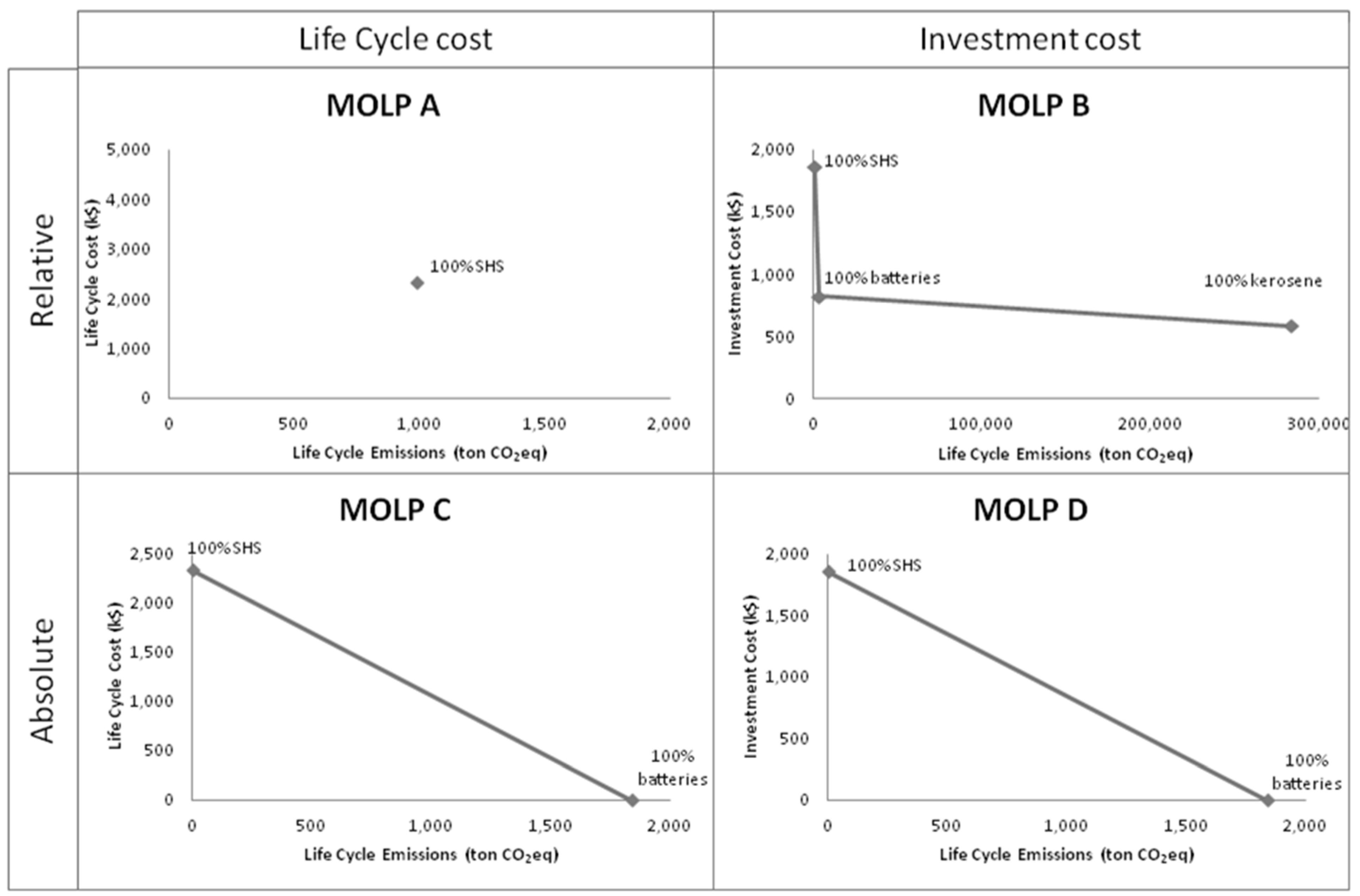
3.3.2. MOLP Optimal Solution Frontiers

An overview of all Pareto optimal solutions for each model is presented in Figure 1. When considering life cycle costs and the relative mitigation cost methodology (MOLP A), we see that the use of solar home systems to fulfill lighting demands represents a single optimal solution from economic and environmental point of view. Said differently, in this case, there is no trade-off between economic and environmental performances, which can also be seen in Table 3. This is in correspondence with the relative mitigation life cycle cost analysis, as the cost of solar LED lanterns (−133.81 $/t CO₂eq) exceeds the mitigation cost of SHS for both baselines (−158.03 and −371.28 $/t CO₂eq). When considering life cycle costs and the absolute mitigation cost methodology (excluding baseline costs) on the other hand, the optimal solution front implies a trade-off between the use of SHS and batteries (MOLP C). The same conclusion is valid when considering investment costs and the absolute mitigation cost methodology (MOLP D). In both cases, the mitigation cost analysis provides ambiguous results when comparing solar LED lanterns and SHS. Moreover, in the absolute life cycle cost analysis (corresponding to MOLP C) the mitigation cost of solar LED lanterns (33.56 $/t CO₂eq) exceeds that of SHS when kerosene is considered as baseline (12.06 $/t CO₂eq) but is smaller than if batteries were the baseline (1269.64 $/t CO₂eq). This is also valid when considering the absolute investment cost analysis (MOLP D); the mitigation cost of solar LEDs (16.31 $/t CO₂eq) lies between that of SHS when the baseline would be kerosene (9.58 $/t CO₂eq) or batteries (1009.72 $/t CO₂eq). When considering merely the cost of investment and the relative mitigation cost methodology (MOLP B), the exclusive use of kerosene lanterns represents the economic lexicographic optimum. A relatively small increase in investment cost (+41%) is required to largely decrease the life cycle emissions (−7456%). To reach the environmental lexicographic optimum (that comprises the sole use of SHS) however, the investment cost requires to be increased with 124% to lower emissions with an additional 278%. Hence, the use of multi-objective optimization allows quantifying the trade-off between economic and environmental performances of the optimal solutions.

Figure 1. Optimal solution frontiers of the multi-objective linear programming (MOLP) models.

Figure 1. Optimal solution frontiers of the multi-objective linear programming (MOLP) models.

3.3.3. The Added Value of Complementing the Mitigation Cost Analysis with Multi-Objective Optimization

The results of the mitigation cost analysis are clear and concise, yet the drawback is that they are highly dependent on the baseline technology. Moreover, the mitigation cost analysis allows ranking technologies in order of increasing cost of emission abatement only if the same baseline technology is assumed to be replaced. If a project technology can replace plural baselines (e.g., SHS can replace kerosene lanterns and batteries), the mitigation cost analysis can lead to ambiguous results. The multi-objective linear programming approach on the other hand—which in this case is very straightforward—allows ranking technologies in order of increasing cost of emission abatement, without requiring a baseline. Considering the aforementioned example, we can see from MOLP B that SHS always outperform solar LED lanterns, as the latter do not appear in the optimal solution frontier. Moreover, the use of multi-objective optimization enables quantifying the trade-off between economic and environmental performances of the optimal technologies. This allows the decision maker to opt for one of these optima based on personal preferences. We note that in our analysis, the solar LED lanterns are never part of the optimal solution frontier; in all cases they are outperformed by SHS.

4. Conclusions and Discussion

The results of this paper encourage the use of relative rather than absolute mitigation costs to assess the attractiveness of CDM projects. This implies that avoided baseline costs are to be taken into account, often rendering the projects economically viable. Due to the inherent CDM structure, however, it is currently more obvious to apply absolute mitigation costs, as project investors do not automatically receive an operational return from implemented rural projects. Consequently, economic viability—which is a necessary condition for project implementation—is not automatically realized. This is a mere structural problem, which can be altered to a win-win situation for both parties by including guidelines to stimulate an additional revenue stream of the avoided baseline costs. Correcting this metric accordingly will especially influence the evaluation of small-scale renewable energy projects, as the avoided costs of fossil fuels render these projects profitable. In case of lighting, this would correspond to a “lighting as a service model”, in which the project developer will pay upfront lighting costs and is compensated through a performance contract, i.e., the energy savings due to the new lighting technology. It has already been demonstrated in literature that these projects make a significant contribution to the sustainability of host countries. When reconsidering the mitigation cost as such, the CDMs twin objectives—i.e., assisting at cost-effective emission reduction and contributing to sustainable development—are more likely to be reconciled rather than opposed. One drawback of the mitigation cost analysis is that results are always dependent on the baseline chosen. In case of plural potential baseline technologies, we stimulate the use of a multi-objective approach. Moreover, multi-objective optimization enables quantifying the trade-off between economic and environmental performances of the optimal technologies, without requiring a baseline.

We note that the mitigation cost does not consider CER credit revenues. Accordingly, a negative mitigation cost—as is the case with rural solar projects—means that the project is viable without CER revenue. A natural interpretation would be to state that the project is not “additional”, i.e., that the emission reduction would have occurred anyways, without registration as a CDM project. However, to demonstrate “additionality” in this case (i.e., to demonstrate that the project wouldn’t have occurred without CDM provisions), barrier analysis should be applied. More specifically, the high investment cost of the solar technologies clearly provides a barrier to widespread market penetration. Besides using the income of CER units to help finance the higher initial purchase price, CER revenues in this case could be used to cover the risk of non-payment of the avoided baseline revenue stream. Our research does not consider energy storage, yet this can be an interesting means for mitigating the variability of renewable electricity sources such as solar PV [34]. This is an interesting topic to include in a more detailed model. Finally, we note that the multi-objective optimization in our analysis might represent a simplification of the studied case. Nevertheless, our analysis is a good start and could be completed by including the economies of scale (i.e., cost advantages that are obtained with increasing scale) using multi-objective mixed integer programming.

References

1. UNFCCC. The Mechanisms under the Kyoto Protocol: Emissions Trading, the Clean Development Mechanism and Joint Implementation. Available online: http://unfccc.int/kyoto_protocol/mechanisms/items/1673.php (accessed on 24 February 2014).
2. UNFCCC. Clean Development Mechanism (CDM). Available online: http://unfccc.int/kyoto_protocol/mechanisms/clean_development_mechanism/items/2718.php (accessed on 14 January 2014).
3. UNFCCC. Benefits of the Clean Development Mechanism 2012. Available online: http://cdm.unfccc.int/about/dev_ben/ABC_2012.pdf (accessed on 14 January 2014).
4. Sutter, C.; Parreno, J.C. Does the current clean development mechanism (CDM) deliver its sustainable development claim? An analysis of officially registered CDM projects. Clim. Chang. 2007, 84, 75–90. [Google Scholar] [CrossRef]
5. Olsen, K.H. The clean development mechanismʼs contribution to sustainable development: A review of the literature. Clim. Chang. 2007, 84, 59–73. [Google Scholar] [CrossRef]
6. Pearson, B. Market failure: Why the clean development mechanism wonʼt promote clean development. J. Clean. Prod. 2007, 15, 247–252. [Google Scholar] [CrossRef]
7. Olsen, K.H.; Fenhann, J. Sustainable development benefits of clean development mechanism projects—A new methodology for sustainability assessment based on text analysis of the project design documents submitted for validation. Energy Policy 2008, 36, 2819–2830. [Google Scholar] [CrossRef]
8. Del Rio, P. Encouraging the implementation of small renewable electricity CDM projects: An economic analysis of different options. Renew. Sustain. Energy Rev. 2007, 11, 1361–1387. [Google Scholar] [CrossRef]
9. Kim, J.E.; Popp, D.; Prag, A. The clean development mechanism and neglected environmental technologies. Energy Policy 2013, 55, 165–179. [Google Scholar] [CrossRef]
10. UNFCCC. Cdm—Project Search. Available online: http://cdm.unfccc.int/Projects/projsearch.html (accessed on 14 January 2014).
11. Yaqoot, M.; Diwan, P.; Kandpal, T.C. Solar lighting for street vendors in the city of dehradun (India): A feasibility assessment with inputs from a survey. Energy Sustain. Dev. 2014, 21, 7–12. [Google Scholar] [CrossRef]
12. Mills, E.; Gengnagel, T.; Wollburg, P. Solar-LED alternatives to fuel-based lighting for night fishing. Energy Sustain. Dev. 2014, 21, 30–41. [Google Scholar] [CrossRef]
13. Lazarus, M.; Heaps, C.; Raskin, P. Long Range Energy Alternatives Planning (LEAP) System. Reference Manual; Boston Stockholm Environment Institute (SEI): Stockholm, Sweden, 1995. [Google Scholar]
14. Sathaye, J.; Meyers, S. Greenhouse Gas Mitigation Assessment: A Guidebook; Kluwer Academic Publishers: Dordrecht, The Netherlands, 1995. [Google Scholar]
15. Steuer, R.E. Multiple Criteria Optimization: Theory, Computation, and Application; John Wiley & Sons, Inc.: New York, NY, USA, 1986. [Google Scholar]
16. Environmental Management—Life Cycle Assessment—Requirements and Guidelines; ISO: Geneva, Switzerland, 2010.
17. European Commission—Joint Research Centre—Institute for Environment and Sustainability, International Reference Life Cycle Data System (ILCD) Handbook—General Guide for Life Cycle Assessment—Detailed Guidance; Publications Office of the European Union: Luxembourg, Luxembourg, 2010.
18. De Schepper, E.; Van Passel, S.; Lizin, S.; Achten, W.M.J.; van Acker, K. Cost-efficient emission abatement of energy and transportation technologies: Mitigation costs and policy impacts for Belgium. Clean Technol. Environ. Policy 2014, 16, 1107–1118. [Google Scholar] [CrossRef]
19. Ehrgott, M. Multicriteria Optimization, 2nd ed.; Springer: Auckland, New Zealand, 2010. [Google Scholar]
20. De Schepper, E.; Van Passel, S.; Lizin, S.; Vincent, T.; Martin, B.; Gandibleux, X. Economic and environmental multi-objective optimisation to evaluate the impact of belgian policy on solar power and electric vehicles. J. Environ. Econ. Policy 2015, 1–27. [Google Scholar] [CrossRef]
21. IEA. Weo-2011 New Electricity Access Database; IEA: Paris, France, 2011. [Google Scholar]
22. IFC. Lighting Asia: Solar off-Grid Lighting Market Analysis of: India, Bangladesh, Nepal, Pakistan, Indonesia, Cambodia, and Philippines; IFC: New Delhi, India, 2012. [Google Scholar]
23. Durlinger, B.; Reinders, A.; Toxopeus, M. A comparative life cycle analysis of low power PV lighting products for rural areas in south east asia. Renew. Energy 2012, 41, 96–104. [Google Scholar] [CrossRef]
24. Harish, S.M.; Raghavan, S.V.; Kandlikar, M.; Shrimali, G. Assessing the impact of the transition to light emitting diodes based solar lighting systems in India. Energy Sustain. Dev. 2013, 17, 363–370. [Google Scholar] [CrossRef]
25. UNFCCC. AMS-I.A.: Electricity Generation by the User—Version 16.0; UNFCCC: Bonn, Germany, 2012. [Google Scholar]
26. UNFCCC. AMS-III.AR: Small-Scale Methodology: Substituting Fuel Based Lighting with LED/CFL Lighting Systems—Version 04.0; UNFCCC: Bonn, Germany, 2012. [Google Scholar]
27. Durlinger, B. Case b: Environmental Impact of Photovoltaic Lighting. In The Power of Design; John Wiley & Sons, Ltd.: Chichester, UK, 2012; pp. 253–262. [Google Scholar]
28. Frischknecht, R.; Jungbluth, N.; Althaus, H.J.; Doka, G.; Heck, T.; Hellweg, S.; Hischier, R.; Nemecek, T.; Rebitzer, G.; Spielmann, M.; et al. Overview and Methodology Ecoinvent Report No. 1; Swiss Centre for Life Cycle Inventories: Dübendorf, Switzerland, 2007. [Google Scholar]
29. Goedkoop, M.; Heijungs, R.; Huijbregts, M.; de Schryver, A.; Struijs, J.; van Zelm, R. Recipe 2008—A Life Cycle Impact Assessment Method Which Comprises Harmonised Category Indicators at the Midpoint and the Endpoint Level. First Edition (Revised); Report I: Characterisation; Ministry of Housing, Spatial Planning and Environment (VROM): The Hague, The Netherlands, 2012. [Google Scholar]
30. UNFCCC. CDM Methodology Booklet; UNFCCC: Bonn, Germany, 2013. [Google Scholar]
31. SceT-Maroc & GERERE. Small-Scale Project Design Document—Photovoltaic Kits to Light up Rural Households in Morocco; SceT-Maroc & GERERE: Rabat, Spain, 2005. [Google Scholar]
32. CDM—Executive Board. Small-Scale Cdm Programme of Activities Design Document Form—Installation of Solar Home Systems in Bangladesh Version 09; CDM—Executive Board: Bonn, Germany, 2012. [Google Scholar]
33. IPCC. IPCC Guidelines for National Greenhouse Gas Inventories; IPCC: Kanagawa, Japan, 2006. [Google Scholar]
34. Beaudin, M.; Zareipour, H.; Schellenberglabe, A.; Rosehart, W. Energy storage for mitigating the variability of renewable electricity sources: An updated review. Energy Sustain. Dev. 2010, 14, 302–314. [Google Scholar] [CrossRef]
35. European Commission. Part III: Annexes to Impact Assessment Guidelines; European Commission: Brussels, Belgium, 2009; p. 71. [Google Scholar]
36. OECD/IEA. Energy Statistics Manual; OECD/IEA: Paris, France, 2004. [Google Scholar]