Equivalent Consumption Minimization Strategy for the Control of Real Driving NOx Emissions of a Diesel Hybrid Electric Vehicle

Abstract

Motivated by the fact that the real driving NO_x emissions (RDE) of conventional diesel vehicles can exceed the legislation norms by far, a concept for the control of RDE with a diesel parallel hybrid electric vehicle (HEV) is proposed. By extending the well-known equivalent consumption minimization strategy (ECMS), the power split degree of freedom is used to control the NO_x emissions and the battery state of charge (SOC) simultaneously. Through an appropriate formulation of the problem, the feedback control is shown to be separable into two dependent PI controllers. By hardware-in-the-loop (HIL) experiments, as well as by simulations, the proposed method is shown to minimize the fuel consumption while tracking a given reference trajectory for both the NO_x emissions and the battery SOC.

1. Introduction

Light-duty diesel vehicles are known for their low fuel consumption, as compared to gasoline vehicles. However, due to legislative restrictions, vehicle manufacturers continuously have to make considerable efforts to reduce the pollutant emissions of diesel vehicles. Although the legislative limits have been continuously reduced over the last decade, the real driving emissions, which are the emissions emitted during every-day driving, can far exceed the legislative limits, even for Euro 6 certified light-duty vehicles, as shown in several studies [1–5]. One reason is that the homologation of the vehicles is performed on well-defined, but unrealistic driving cycles. The manufacturers unavoidably focus the optimization effort on such types of vehicle operating conditions. To reduce the discrepancy between the certified and the real-world pollutant emissions, the European commission is currently discussing measures to limit real driving emissions [5].

One option to cope with such a radical change would be to continuously monitor and control the pollutant emissions by an appropriate exhaust aftertreatment system. Another option is provided by electric hybridization of the vehicles, which not only offers a reduction of pollutant emissions, but also a simultaneous reduction of the CO₂ emissions. Since hybrid electric vehicles (HEVs) have an additional degree of freedom for the control of the energy flows in the powertrain, the trade-off between fuel consumption and pollutant emissions can be further influenced.

Some studies can be found in the literature about the control of pollutant emissions for HEVs. For example, the authors of [6] propose a real-time rule-based strategy to optimize both fuel economy and pollutant emissions, taking into account cold-start emissions, by minimizing an overall normalized impact function. Similar approaches have been presented in [7–11], where an instantaneous optimization algorithm, with a similar structure to the well-known equivalent consumption minimization strategy (ECMS) [12,13], is built. In that case, the target is to minimize a weighted sum of multiple factors, for example fuel consumption and NO_x, CO and CO₂ emissions, while guaranteeing charge-sustaining conditions for various driving cycles. The weighting factors between the various components of the target cost function are constant and considered to be tuning parameters. For a diesel HEV equipped with a selective catalytic reaction (SCR) system, a noncausal extended ECMS is proposed in [14], including the minimization of tailpipe emissions, while considering the cold start behavior. A control framework with three state variables arises from the energy management extended with emissions management; these are the energy stored in the battery, the SCR catalyst temperature and total NO_x tailpipe mass, resulting in a controller with an unstable co-state, which can be used in a fixed time window only.

Dynamic programming (DP) has also been applied to address the problem of building a supervisory control system for the fuel and emission reduction. Examples are given in [15,16] for a parallel HEV, where the gearshift strategy and the engine start/stop decision are optimized along with the torque split factor and, in [17], considering the power split as the only control input. In both studies, constant weighting factors for the multiple emission sources have been applied.

A general approach based on optimal control theory is proposed in [18], with a description of several possible extensions of the basic framework of ECMS. The authors describe how to include different pollutant components for an HEV, possibly taking into consideration thermal effects and aftertreatment systems. The authors claim that the solution of such a general problem is not available yet. Emissions can also be included in map-based ECMS approaches, as suggested in [19]. An experimental validation of a method based on a constant weighting factor for NO_x emissions has been provided in [20] by means of hardware-in-the-loop (HIL) experiments.

Other studies focus on the control of transient emissions, especially regarding hybrid powertrains relying on a diesel combustion engine. An optimal energy management strategy is provided by the authors of [21] with a DP approach for constant weighting factors related to NO_x and particulate emissions. A key idea for the energy management strategy of a diesel HEV is to use the electric motor for torque phlegmatization during transients, for example by adopting heuristic methods, as presented in [22,23], or model-based frameworks, as reported in [24–26].

However, a control strategy that includes online adaptation of the weighting factors for the objective pollutant emission, to take into account real-world driving conditions and a possible modification of the emissions target level, has not been demonstrated yet. Therefore, in this paper, an energy management strategy that allows for the tracking of a specific NO_x emission level to respect real driving emission constraints is presented. Under these conditions, the strategy is constructed to minimize the fuel consumption while sustaining the battery state of charge (SOC).

The paper is structured as follows: after explaining the vehicle model in detail in Section 2; the energy management strategy, which takes into account the real driving emissions, is derived in Section 3; then, Section 4 presents an experimental validation of the method proposed, as well as a simulation case study that quantifies the fuel savings potential compared to a standard method not accounting for real driving emissions.

2. Vehicle Model

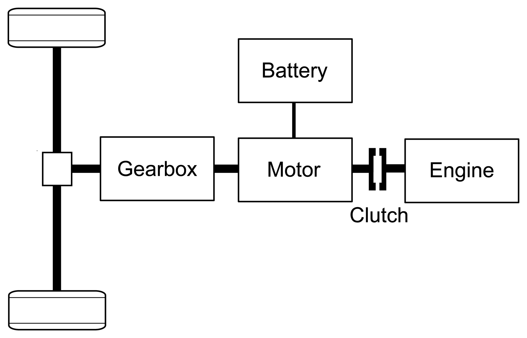
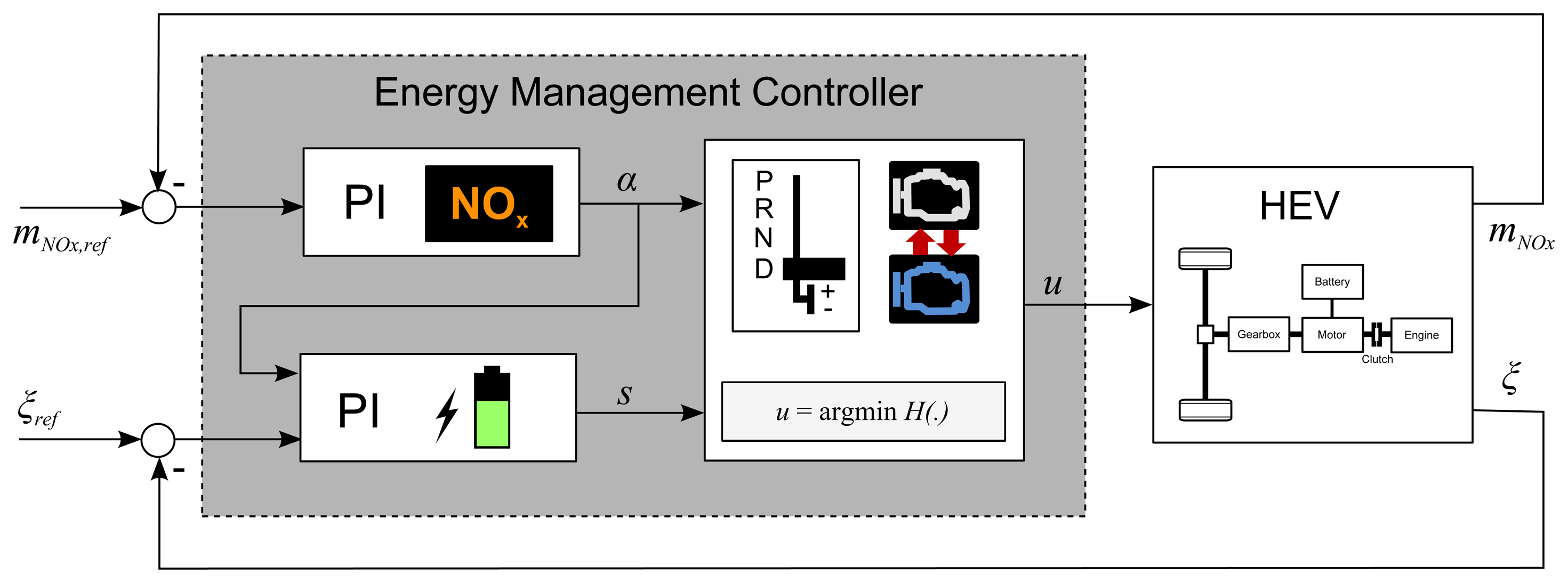
The vehicle under investigation is a fictitious executive class sedan. The powertrain architecture is of the pre-transmission parallel type, as illustrated in Figure 1. The powertrain consists of a seven-step automatic gearbox, a 40 kW electric motor, the power electronics, a 2 kW h battery, a clutch and a 170 kW diesel engine. For the simulation of the vehicle behavior, only the longitudinal dynamics of the vehicle are of interest, since the consideration of these dynamics is sufficient for energetic considerations [27]. The longitudinal dynamics are simulated using a so-called forward approach, in which the physical causality is respected. By contrast, for the energy management of the powertrain, a model-based approach is chosen, in which the powertrain behavior is predicted by a so-called backward approach, where the physical causality is inverted [27].

More details on the modeling of the vehicle are given in the following. All the values needed to parameterize the model are listed in

Table 1. Nominal data of the vehicle and of the powertrain components. SOC: state of charge.

Parameter	Symbol	Value
Wheel radius	rw	0.32 m
Air density	ρair	1.24 kg/m3
Effective frontal area	cd · A	0.60 m2
Rolling friction coefficient	cr	0.012
Gravitational constant	ag	9.81 m/s2
Total vehicle mass	mv	1827 kg
Total inertia of the wheels	Θw	4.78 kg m2
Inertia of the motor	Θm	0.0435 kg m2
Gear ratios	ig	[10.8, 7.1, 4.7, 3.4, 2.5, 2.0, 1.8]
Gearbox efficiency parameter	ηg,0	0.95
	ηg,1	0.02 1/(rad/s)
	ωg,1	400 rad/s
Nominal motor power	-	40 kW
Maximum motor speed	ωm,max	628 rad/s
Nominal engine power	-	170 kW
Minimum engine speed	ωe,min	105 rad/s
Maximum engine speed	ωe,max	471 rad/s
Maximum battery capacity	Q0	7.64 A h
Open circuit voltage	Voc	263 V
Battery internal resistance	Ri	0.24 Ω
Minimum battery current	Ib,min	−166 A
Maximum battery current	Ib,max	229 A
Minimum SOC	SOCmin	0.20
Maximum SOC	SOCmax	0.80
Auxiliary power demand	Paux	400 W

.

2.1. Longitudinal Dynamics

The equation for the longitudinal dynamics of the vehicle is described by [27]:

$$\frac{\text{d}v(t)}{\text{d}t}=\frac{1}{m(t)}\cdot \left(\frac{T_{\text{w}}(t)}{r_{\text{w}}}-\frac{1}{2}{\rho }_{\text{air}}{c}_{\text{d}}A{v}^2(t)-c_{\text{r}}{m}_{\text{v}}{\text{a}}_{\text{g}}cos(\gamma (t))-m_{\text{v}}{\text{a}}_{\text{g}}sin(\gamma (t))\right)$$

(1)

with:

$$m(t)=m_{\text{v}}+\frac{{\Theta }_{\text{w}}}{r_{\text{w}}^2}+\frac{{\Theta }_{\text{EM}}{i}_{\text{g}}^2(t)}{r_{\text{w}}^2}$$

(2)

where v denotes the vehicle speed; T_w denotes the wheel torque; r_w denotes the wheel radius; ρ_air denotes the air density; c_d denotes the aerodynamic drag coefficient; A denotes the frontal area of the vehicle; c_r denotes the rolling friction coefficient; m_v denotes the nominal vehicle weight; Θ_w and Θ_EM denote the inertia of the four wheels and the electric motor, respectively; a_g denotes the gravitational acceleration; and γ denotes the road slope.

2.2. Gearbox Model

The rotational speed of the gearbox input shaft, ω_g, is given by:

$${\omega }_g(t)=\frac{v(t)}{r_{\text{w}}}\cdot i_g(t)$$

(3)

where i_g is the gear ratio of the gear engaged, g ∈ {1,…, 7}. The gear engaged, g, is decided by the gear decision variable, u_g, defined by the energy management. For simplicity, the gearshifts are assumed to occur instantaneously without any delays.

The torque delivered to the wheels, T_w, is calculated by:

$$T_{\text{w}}(t)=T_g(t)\cdot i_g(t)\cdot {\left({\eta }_{g,0}-\frac{{\eta }_{g,1}}{{\omega }_{g,1}}\cdot {\omega }_g(t)\right)}^{\text{sign}(T_g(t))}$$

(4)

with T_g being the input torque of the gearbox; and η_g,0, η_g,1, ω_g,1 being the parameters to model the speed-dependent gearbox losses, which account for the increased friction at higher gearbox input speeds [28]. The values for the efficiency parameters are chosen based on expert knowledge.

The input torque of the gearbox is:

$$T_g(t)=T_{\text{m}}(t)+u_{\text{c}}(t)\cdot T_{\text{e}}(t)$$

(5)

where T_m is the motor torque; T_e is the engine torque; and u_c is the clutch state command determined by the energy management. The value u_c = 1 means that the clutch is closed, and the value u_c = 0 means that the clutch is open. The clutch command is assumed to be realized instantaneously.

2.3. Electric Motor Model

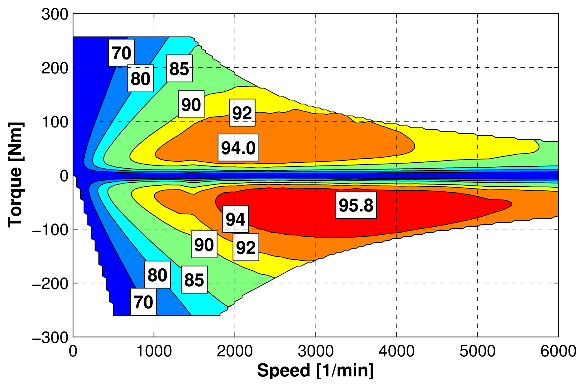
The desired torque for the electric motor, determined by the energy management, is assumed to be realized instantaneously without any delays. The power of the electric motor, including the power electronics, is given by a steady-state efficiency map, depicted in Figure 2, so that:

$$P_{\text{m}}(t)=f_{\text{m}}\left({\omega }_{\text{m}}(t),T_m(t)\right)$$

(6)

The minimum and maximum torque values for the electric motor, as well as the minimum and maximum speeds are defined by:

$$0\le {\omega }_{\text{m}}(t)\le {\omega }_{\text{m},max}$$

(7)

$$T_{\text{m},min}({\omega }_{\text{m}}(t))\le T_{\text{m}}(t)\le T_{m,\text{max}}({\omega }_{\text{m}}(t))$$

(8)

2.4. Engine Model

The desired torque of the engine is determined by the energy management. However, the rate of change of the engine torque is limited by 100 N m/s in order to prevent the formation of excessive soot and NO_x emissions during transients [23,31].

The rotational speed of the engine, ω_e, is defined by (for brevity, the notation of time is omitted):

$${\omega }_{\text{e}}=\{\begin{array}{ll}0\hfill & \text{if}{u}_{\text{e}}=u_{\text{c}}=0,\hfill \\ {\omega }_{\text{e},\text{idle}}\hfill & \text{if}(u_{\text{e}}=1\text{and}{u}_{\text{c}}=0)\text{or if}(u_{\text{e}}=u_{\text{c}}=1\text{and}{\omega }_g<{\omega }_{\text{e},\text{idle}})\hfill \\ {\omega }_g\hfill & \text{if}(u_{\text{e}}=u_{\text{c}}=1\text{and}{\omega }_g\ge {\omega }_{\text{e},\text{idle}})\text{or if}(u_{\text{e}}=0\text{and}{u}_{\text{c}}=1)\hfill \end{array}$$

(9)

where u_e is the engine on/off command, with 0 standing for “off” and 1 standing for “on”; and u_c is the clutch state command, with 0 standing for “open” and 1 standing for “closed”.

The mass flow rate of the fuel consumed, ${\stackrel{*}{m}}_{\text{fuel}}$, and NO_x emissions, ${\stackrel{*}{m}}_{N{O}_x}$, are calculated using measured steady-state maps in the form of:

$${\stackrel{*}{m}}_{\text{fuel}}(t)=f_{\text{e},\text{fuel}}\left({\omega }_{\text{e}}(t),T_{\text{e}}(t)\right)$$

(10)

$${\stackrel{*}{m}}_{N{O}_x}(t)=f_{e,N{O}_x}\left({\omega }_e(t),T_e(t)\right)$$

(11)

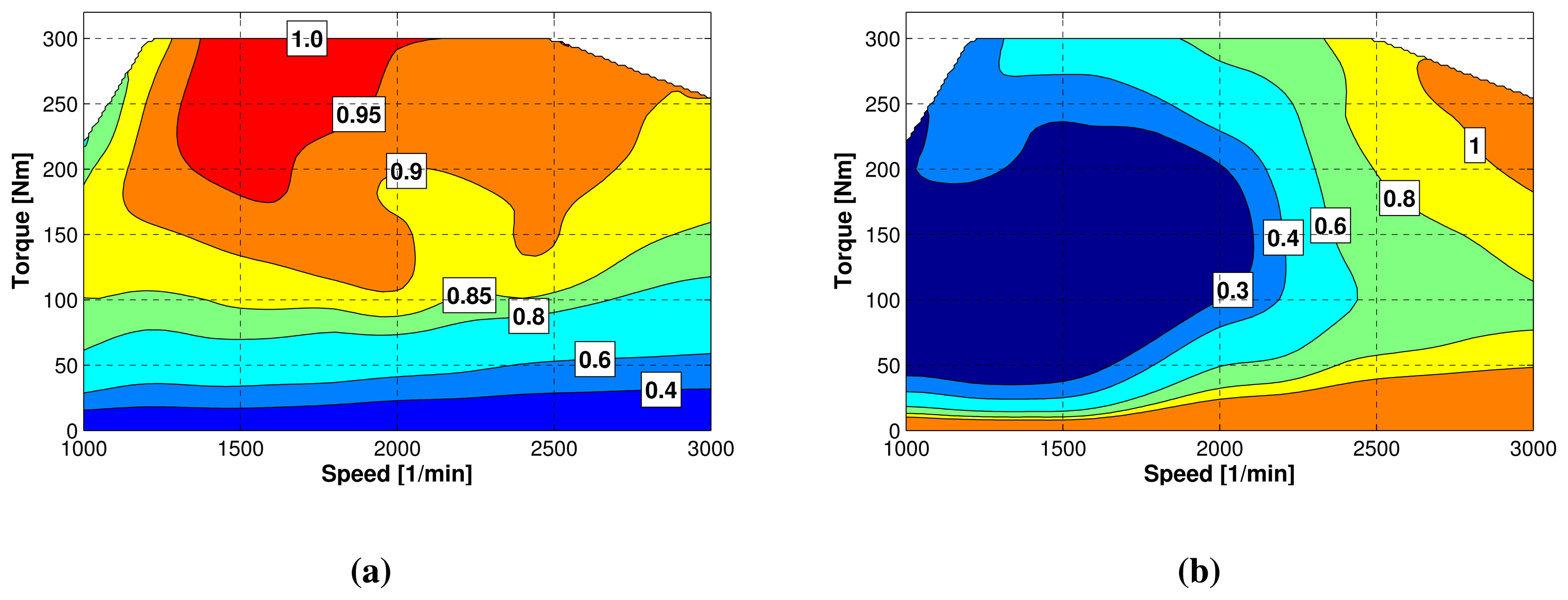
The map for the fuel efficiency and the map for the NO_x emissions are shown in Figure 3.

At all times, the engine is only allowed to operate within its limits, defined by maximum torque and speed range conditions, i.e.,

$${\omega }_{\text{e},min}(t)\le {\omega }_{\text{e}}(t)\le {\omega }_{\text{e},max}$$

(12)

$$0\le T_{\text{e}}(t)\le T_{\text{e}}\left({\omega }_{\text{e}}(t)\right)$$

(13)

2.5. Battery Model

The battery is modeled as an equivalent circuit with a constant open-circuit voltage, V_oc, in series with a constant internal resistance, R_i [27]. Since the battery is assumed to be of the LiFePO₄ type [32,33], the assumption of a constant open-circuit voltage is a valid approximation for the typical operating range of the battery [34–36].

The equation of the dynamics of the battery SOC, ξ, is given by:

$$\frac{\text{d}\xi (t)}{\text{d}t}=-\frac{I_{\text{b}}(t)}{Q_0}$$

(14)

with:

$$I_{\text{b}}(t)=\frac{V_{\text{oc}}(\xi (t))-\sqrt{V_{\text{oc}}^2(\xi (t))-4R_i(P_{\text{m}}(t)+P_{\text{aux}})}}{2\cdot R_i(\xi (t))}$$

(15)

where I_b is the battery current, and P_aux is a constant power consumed by electric auxiliary units. Although in this paper, V_oc and R are assumed to be constant, the notation for the dependency on the SOC is preserved to keep the following derivation of the causal controller more general.

The battery current and the battery SOC are constrained to:

$$I_{\text{b},min}\le I_{\text{b}}(t)\le I_{\text{b},max}$$

(16)

$${\xi }_{min}\le \xi (t)\le {\xi }_{max}$$

(17)

respectively.

2.6. Driver

The driver model consists of a proportional-integral (PI) controller. The output of the model is a preliminary throttle position, θ̃, calculated by:

$$\tilde{\theta }(t)=k_{\text{p},\text{D}}\cdot \left(v_{\text{ref}}(t)-v(t)\right)+\frac{1}{T_{i,\text{D}}}\cdot {\int }_0^t\left(v_{\text{ref}}(\tau )-v(\tau )\right)\text{d}\tau$$

(18)

with k_p,D and T_I,D being the proportional and integral controller parameters with the manually tuned values of 0.9 and 11 s, respectively. The final throttle position, θ, is then obtained by saturating the preliminary throttle signal as follows:

$$\tilde{\theta }(t)=\{\begin{array}{ll}100\hfill & \text{if}\tilde{\theta }(t)>100\hfill \\ \tilde{\theta }\hfill & \text{if}-100\le \tilde{\theta }(t)\le 100\hfill \\ -100\hfill & \text{if}\tilde{\theta }(t)<-100\hfill \end{array}$$

(19)

Due to the saturation and the integral control part of the driver model, an anti-windup scheme is implemented [37].

The mapping of the throttle position, θ, to a desired torque command, T_req, is designed, such that:

• θ = 100% corresponds to the maximum possible traction torque provided by both the engine and the motor at the current vehicle speed;

• θ = 0% corresponds to a zero torque request; and

• θ = −100% corresponds to the maximum possible brake torque.

The intermediate torque commands are obtained by linear interpolation of the throttle position.

2.7. Energy Management

The energy management defines the set points for the gear number to be engaged, u_g, the clutch open/closed state, u_c, the engine on/off state, u_e, and the torque split, u_ts, between the engine and the motor.

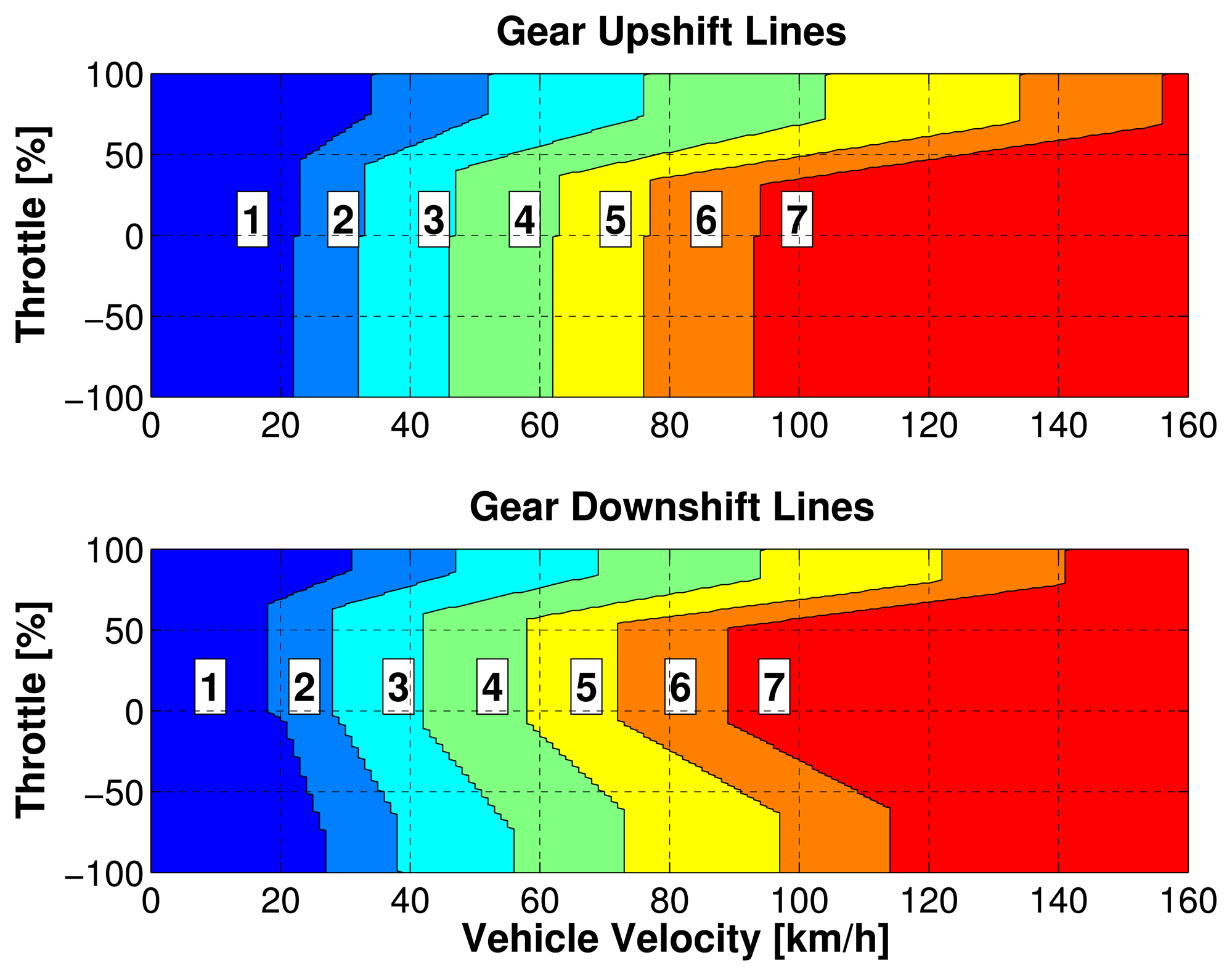
The gear command, u_g, is determined by a lookup table of the form:

$$u_g(t)=f_g\left(v(t),\theta (t)\right)$$

(20)

as shown in Figure 4. The figure shows the upshift and downshift lines depending on the vehicle velocity, v, and the throttle position, θ. For comfort reasons, after every gear change, the new gear has to remain in its state for at least 3 s before another gear can be engaged. This time-based hysteresis can only be overruled in the case the throttle is fully depressed.

The clutch command, u_c, is defined as follows: if the engine is off, the clutch is assumed to be open. If the engine is on and the desired engine torque is larger than zero, the clutch is closed. Otherwise, if the engine is on and the desired engine torque is equal to zero, the clutch is open, and the engine is assumed to be running idle.

The torque split, u_ts, is defined as the ratio of the motor torque and the requested torque from the driver:

$$u_{\text{ts}}=\frac{T_{\text{m}}}{T_{\text{req}}}$$

(21)

Then, the torques of the motor and the engine are obtained by:

$$T_{\text{m}}=T_{\text{req}}\cdot u_{\text{ts}}$$

(22)

$$T_{\text{e}}=T_{\text{req}}\cdot \left(1-u_{\text{ts}}\right)$$

(23)

Recharging during standstill is not considered here; however, this feature could be implemented easily.

The commands for the engine on/off, u_e, and the torque split, u_ts, are determined by an online optimization method commonly known as the ECMS [12,13,34]. To account for the diesel exhaust emissions, the standard approach has been extended, as shown in Section 3 below.

3. Controller

This section presents a detailed description of the controller developed to optimize the fuel consumption of a diesel hybrid vehicle under a constraint for the NO_x emissions. The description of the control system is given in Section 3.1, while the solution of the control problem, derived by means of optimal control theory, is provided in Section 3.2. Then, Section 3.3 proposes a derivation of a causal online controller. To implement such a controller, the dependency between the co-states must be identified, which is illustrated in Section 3.6. The final structure of the controller is shown in Section 3.7, and the assignment of the corresponding reference signal trajectories is described in Section 3.8.

3.1. System Description

The hybrid vehicle system can be described by a system of first-order ordinary differential equations:

$$\frac{\text{d}}{\text{d}t}x(t)=f\left(x(t),u(t)\right)$$

(24)

where x is the state vector and u the control input vector. The state and the control input vector are:

$$\begin{array}{cc}x(t)=\left[\begin{array}{c}\xi (t)\\ m_{N{O}_x}(t)\end{array}\right],& u(t)=\left[\begin{array}{c}{u}_{\text{e}}(t)\\ u_{\text{ts}}(t)\end{array}\right]\end{array}$$

(25)

where ξ is the battery SOC, m_NOx the cumulated NO_x emissions, u_e the engine on/off command and u_ts the torque split command, as previously introduced in Section 2.7. The control input for the gear number, u_g, is decided independently of x and u, and the control input for the clutch state, u_c, is defined by a known function of u_e. Therefore, u_g and u_c are not subject to optimization and, hence, not included in u.

Notice that the vehicle speed is not considered to be a state variable, because the speed is assumed to be perfectly tracked. Based on the actual vehicle speed and the driver's torque request, the required torques and the shaft speeds can be determined using a backwards calculation [27].

Using these definitions, the model for the system dynamics is derived based on the description presented in the previous section. The state dynamics equations become:

$$\frac{\text{d}}{\text{d}t}x(t)=f(x(t),u(t))=\left[\begin{array}{c}\frac{\text{d}}{\text{d}t}\xi \left(x(t),u(t)\right)\\ \frac{\text{d}}{\text{d}t}{m}_{N{O}_x}\left(x(t),u(t)\right)\end{array}\right]=\left[\begin{array}{c}-\frac{I_{\text{b}}(\xi (t),u(t))}{Q_0}\\ {\stackrel{*}{m}}_{N{O}_x}(u(t))\end{array}\right]$$

(26)

The choice for the integral of the emissions as a state variable has an advantage compared to the specific emission level, as defined in legislation as:

$${\overline{m}}_{N{O}_x}=\frac{m_{N{O}_x}}{d}$$

(27)

with d being the distance driven. The derivative of the latter expression would be:

$$\begin{array}{ll}\frac{\text{d}}{\text{d}t}{\overline{m}}_{N{O}_x}\hfill & =\frac{\frac{\text{d}}{\text{d}t}{m}_{N{O}_x}\cdot d-m_{N{O}_x}\cdot v}{d^2}\hfill \\ & =\frac{1}{d}\cdot \left(\frac{\text{d}}{\text{d}t}{m}_{N{O}_x}-{\overline{m}}_{N{O}_x}\cdot v\right)\hfill \end{array}$$

(28)

with v being the vehicle speed. The derivative of the absolute cumulated emissions, m_NOx, is:

$$\frac{\text{d}}{\text{d}t}{m}_{N{O}_x}={\stackrel{*}{m}}_{N{O}_x}$$

(29)

where ${\stackrel{*}{m}}_{N{O}_x}$ denotes the NO_x mass flow rate. The following properties hold:

$$\frac{\partial \left(\frac{\text{d}}{\text{d}t}{\overline{m}}_{N{O}_x}\right)}{\partial {\overline{m}}_{N{O}_x}}=-\frac{v}{d}\ne 0$$

(30)

$$\frac{\partial \left(\frac{\text{d}}{\text{d}t}{m}_{N{O}_x}\right)}{\partial m_{N{O}_x}}=0$$

(31)

These properties play a role in the following derivation.

3.2. Solution Using Pontragin's Minimum Principle (PMP)

According to the general methodology introduced in [38], the problem can be defined as an optimal control problem with partially constrained final states. The problem is formulated as:

$$\underset{u}{min}\left\{J(u)={\int }_0^T{\stackrel{*}{m}}_{\text{fuel}}(u(t))dt\right\}$$

(32)

such that:

$$x(0)=x_0$$

(33)

$$\begin{array}{cc}\frac{\text{d}}{\text{d}t}x(t)=f(x(t),u(t))& \text{for all}t\in [0,T]\end{array}$$

(34)

$$x(T)\in S$$

(35)

The closed final-time set, S, describes the constraints for the final state vector: m_NOx has an upper constraint, since it has to be below a certain emission level, while ξ has to satisfy the charge-sustaining condition for the battery.

The optimal solution is found using Pontryagin's minimum principle (PMP) [38,39]. By defining the Hamiltonian function as:

$$H(x(t),u(t),\lambda (t))={\stackrel{*}{m}}_{\text{fuel}}(u(t))-{\lambda }^T(t)\cdot f(x(t),u(t))$$

(36)

with λ denoting the co-state vector, the optimal solution (denoted by ^o) must satisfy the following conditions:

$$x(0)=x_0$$

(37)

$$\frac{\text{d}}{\text{d}t}{x}^o(t)={\nabla }_{\lambda }{H}_{|o}=f\left(x^0(t),u^o(t)\right)$$

(38)

$$\begin{array}{ll}\frac{\text{d}}{\text{d}t}{\lambda }^o(t)\hfill & =-{\nabla }_x{H}_{|o}\hfill \\ & =-{\nabla }_x{\stackrel{*}{m}}_{\text{fuel}}(u^o(t))-{\left[\frac{\partial f}{\partial x}(x^o(t),u^o(t))\right]}^T\cdot {\lambda }^o(t)\hfill \end{array}$$

(39)

The co-state vector must stay within the normal cone, T*, of the target set, S, at the final time for x^o(T):

$${\lambda }^o(T)\in T*(S,x^o(T))$$

(40)

The Hamiltonian of the system must be minimized for all times with respect to all admissible inputs u, such that:

$$H(x^o(t),u^o(t),{\lambda }^o(t))\le H(x(t),u(t),\lambda (t))$$

(41)

The dynamics of the co-states can be rewritten, separating the battery SOC and the cumulated NO_x co-states, as follows (where the dependencies on the inputs and the states are omitted):

$$\left[\begin{array}{c}\frac{d}{dt}{\lambda }_{\xi }^o(t)\\ \frac{d}{dt}{\lambda }_{N{O}_x}^o(t)\end{array}\right]=\left[\begin{array}{c}-\frac{\partial {\stackrel{*}{m}}_{\text{fuel}}}{\partial \xi }-{\left[\frac{\partial f}{\partial \xi }\right]}^T\cdot {\lambda }^o(t)\\ -\frac{\partial {\stackrel{*}{m}}_{\text{fuel}}}{\partial m_{N{O}_x}}-{\left[\frac{\partial f}{\partial m_{N{O}_x}}\right]}^T\cdot {\lambda }^o(t)\end{array}\right]$$

(42)

Since the fuel mass flow and the NO_x emissions do not explicitly depend on the battery SOC, the equations hold:

$$\frac{\partial {\stackrel{*}{m}}_{\text{fuel}}(u(t))}{\partial \xi }=0$$

(43)

$$\frac{\partial f(x(t),u(t))}{\partial \xi }=\left[\begin{array}{c}-\frac{\partial }{\partial \xi }\frac{I_b(\xi (t),u(t))}{Q_0}\\ 0\end{array}\right]$$

(44)

Moreover, since neither the system dynamics nor the fuel mass flow depend explicitly on the cumulated NO_x emissions, the following expressions hold:

$$\frac{\partial {\stackrel{*}{m}}_{\text{fuel}}(u(t))}{\partial m_{N{O}_x}}=0$$

(45)

$$\frac{\partial f(x(t),u(t))}{\partial m_{N{O}_x}}=\left[\begin{array}{c}0\\ 0\end{array}\right]$$

(46)

Combining Equations (43)–(46) with Equation (42) leads to the following rewritten expression for the co-states dynamics:

$$\left[\begin{array}{c}\frac{\text{d}}{\text{d}t}{\lambda }_{\xi }^o(t)\\ \frac{\text{d}}{\text{d}t}{\lambda }_{N{O}_x}^o(t)\end{array}\right]=\left[\begin{array}{c}\frac{\partial }{\partial \xi }\frac{I_{\text{b}}\xi (t),u(t)}{Q_0}\cdot {\lambda }_{\xi }(t)\\ 0\end{array}\right]$$

(47)

The importance of the choice of cumulated emissions is here demonstrated, since the term, $\frac{\partial f}{\partial m_{N{O}_x}}$, would not have vanished with the choice of specific NO_x emissions as a state variable Equation (30). Further, considering Equation (47) and that ${\lambda }_{N{O}_x}^o(T)\ge 0$, we have that:

$${\lambda }_{N{O}_x}^o=\mathit{\text{const}}.={\lambda }_{N{O}_x}\ge 0$$

(48)

The Hamiltonian in Equation (36) can be rewritten, having defined λ_NOx:

$$\begin{array}{ll}H(\cdot )\hfill & ={\stackrel{*}{m}}_{\text{fuel}}(u(t))-{\lambda }^T(t)\cdot f(x(t),u(t))\hfill \\ & ={\stackrel{*}{m}}_{\text{fuel}}(u(t))+{\lambda }_{N{O}_x}\cdot {\stackrel{*}{m}}_{N{O}_x}(u(t))-{\lambda }_{\xi }(t)\cdot \frac{I_b\left(\xi (t),u(t)\right)}{Q_0}=:\tilde{H}(\cdot )\hfill \end{array}$$

(49)

The latter new expression for the Hamiltonian in Equation (49) leads to a new Hamiltonian, H̃, for the system for the minimization of a weighted sum of fuel and emissions. This leads to a new problem definition:

$$\underset{u}{min}\left\{\tilde{J}(u)={\int }_0^T\left({\stackrel{*}{m}}_{\text{fuel}}(u(t))+{\lambda }_{N{O}_x}\cdot {\stackrel{*}{m}}_{N{O}_x}(u(t))\right)dt\right\}$$

(50)

such that:

$$\xi (0)={\xi }_0$$

(51)

$$\begin{array}{cc}\frac{d}{dt}\xi (t)=-\frac{I_b(\xi (t),u(t))}{Q_0}& \text{for all}t\in [0,T]\end{array}$$

(52)

$$\xi (T)={\xi }_0$$

(53)

For the reformulated optimization problem, λ_NOx is not a co-state but a weighting factor and, therefore, a given parameter. It quantifies the fuel equivalent of a given amount of NO_x emissions, in a new Lagrangian reformulation. For this reason, the authors of [40] have defined the Equations (50)–(53) equivalent emissions minimization strategy (EEMS). The equivalence of the minimization Equations (50)–(53) to the previous Equations (32)–(35) is guaranteed, since the eliminated state does not appear in any of the other equations, and it is introduced only to enforce the limit on cumulated emissions with a final-state constraint. As a consequence, if the constant equivalence factor is known, the same optimal results will be achieved for the redefined problem. As a matter of fact, such value is not known a priori. For this reason, a causal controller based on the online calculation of the equivalence factor is proposed in the following section.

3.3. Emissions and Charge-Sustaining Causal Control

The objective of this section is to present a feedback controller derived for online control of the cumulative NO_x emissions. Before deriving the proposed causal control framework, the cost functional in Equation (50) is conveniently rearranged by introducing the normalized NO_x mass flow rate, ${\widetilde{\stackrel{*}{m}}}_{N{O}_x}$:

$${\widetilde{\stackrel{*}{m}}}_{N{O}_x}(t)={\stackrel{*}{m}}_{N{O}_x}(t)\cdot \frac{{\stackrel{*}{m}}_{N{O}_{x,\mathit{\text{MAX}}}}}{{\stackrel{*}{m}}_{{\text{fuel}}_{\mathit{\text{MAX}}}}}$$

(54)

such that:

$$\overline{J}(u)={\int }_0^T\left({\stackrel{*}{m}}_{\text{fuel}}\left(u(t)\right)+{\lambda }_{N{O}_x}\cdot {\widetilde{\stackrel{*}{m}}}_{N{O}_x}\left(u(t)\right)\right)dt$$

(55)

where the normalization takes place using the maximum flow rates of fuel and NO_x for the given experimental maps of the combustion engine. By means of the rewritten cost functional in Equation (55), the argument of the object function and the corresponding Hamiltonian are expressed by homogenous measuring units.

To achieve the goal of generating a charge and emissions sustaining strategy, two terms can be added to Equation (55) in order to penalize deviations from reference values for SOC, ξ_ref, and deviations from the reference values for the normalized cumulated emission, m̃NO_x,_ref, thus obtaining a new formulation for the cost functional:

$$\widehat{J}(u)={\int }_0^T\widehat{L}\left(x(t),u(t)\right)dt$$

(56)

$$={\int }_0^T\left({\stackrel{*}{m}}_{\text{fuel}}(u(t))+\mu \cdot {\left(\frac{{\tilde{m}}_{N{O}_x,\text{ref}}(t)-{\tilde{m}}_{N{O}_x}(t)}{\mathrm{\Delta }{\tilde{m}}_{N{O}_x,\text{norm}}}\right)}^{2q}+\beta \cdot {\left(\frac{{\xi }_{\mathit{\text{ref}}}(t)-\xi (t)}{\mathrm{\Delta }{\xi }_{\text{norm}}}\right)}^{2p}\right)dt$$

(57)

The extended cost Equation (57) leads to the extended Hamiltonian:

$$\widehat{H}(u)={\stackrel{*}{m}}_{\text{fuel}}(u)+\mu \cdot {\left(\frac{{\tilde{m}}_{N{O}_x,\text{ref}}(t)-{\tilde{m}}_{N{O}_x}(t)}{\mathrm{\Delta }{\tilde{m}}_{N{O}_x,\text{norm}}}\right)}^{2q}+\beta \cdot {\left(\frac{{\xi }_{\text{ref}}(t)-\xi (t)}{\mathrm{\Delta }{\xi }_{\text{norm}}}\right)}^{2p}+{\lambda }^T\cdot f(x,u)$$

(58)

which must be minimized by the optimal input sequence:

$$u^o=\text{argmin}\left(\widehat{H}(u)\right)$$

(59)

Since the additional terms of the extended Hamiltonian do not explicitly depend on the control inputs, they will be minimized by the optimal policy, u^o, as well.

To calculate the co-state dynamics, λ, the Hamilton–Jacobi–Bellman equations provide the following expression [39] for the optimal co-states vector, λ^o:

$${\lambda }^o(x,t)=\frac{\partial {\widehat{C}}^o(x,t)}{\partial x}$$

(60)

where Ĉ^o(x,t) denotes the optimal cost-to-go function associated with the cost function, ĵ(u). The optimal cost-to-go function for the state, x, at the time, t, is given by:

$${\widehat{C}}^o(x,t)=\underset{u}{min}\left\{\begin{array}{cc}{\int }_t^T\widehat{L}(x(\tau ),u(\tau ))d\tau & |x(t)=x\end{array}\right\}$$

(61)

Since the optimal cost-to-go is not known a priori in a causal setting, the optimal cost-to-go function is estimated by a sub-optimal time-invariant function, formed by the sum of different independent cost indices, as follows [41]:

$$\begin{array}{ll}\widehat{C}(x)\hfill & =\widehat{C}(\xi ,{\tilde{m}}_{N{O}_x})=\hfill \\ & ={\widehat{C}}_{f_1,N{O}_x}({\tilde{m}}_{N{O}_x})+{\widehat{C}}_{f_1,\xi }(\xi ,{\tilde{m}}_{N{O}_x})+{\tilde{C}}_{f_2}+{\tilde{C}}_{\xi }(\xi )+{\tilde{C}}_{{\tilde{m}}_{N{O}_x}}({\tilde{m}}_{N{O}_x})\hfill \end{array}$$

(62)

The five terms are explained in the following:

• Ĉ_f1,ξ(ξ,m̃NO_x): the additional fuel consumption caused by compensating for the current SOC deviation;

• Ĉ_f1,_NOx(m̃NO_x): the additional fuel consumption caused by bringing the cumulated NO_x close to the reference level;

• C̃_f2: a fuel consumption that is supposed to be independent of both the current SOC and the current emission level, needed to drive the rest of the driving mission with correct reference values;

• C̃_ξ(ξ): denotes the penalty for SOC deviations from the reference value;

• C̃m(̃_NOx)(m̃NO_x): denotes the penalty of m̃_NOx deviations from the reference value.

3.3.1. Cost of Sustaining the Battery SOC Ĉ_f1,_ξ(ξ, m̃_NOx)

Following the approach described in [41,42], the fuel energy used to compensate for the SOC deviations from the target value can be approximated by first estimating the energy stored in the battery at a certain ξ(t) with respect to the reference, ξ_ref(t), as:

$$E_{\text{BT},\mathrm{\Delta }\xi }=Q_0{\int }_{\xi (t)}^{{\xi }_{\text{ref}}(t)}{V}_{\text{oc}}(\tilde{\xi })d\tilde{\xi }$$

(63)

Since in the future, this energy must be compensated for using the thermal path, a certain amount of fuel will be saved/consumed to discharge/charge the battery. Such a quantity will clearly depend on the future efficiencies of the engine and the electric path, which, in turn, depend on the future engine operating points. Moreover, the used engine operating points will also depend on the cumulated NO_x emissions, since a second controller acts in parallel, modifying the choice of control inputs to track the desired emissions level. As a consequence, the average future charging/discharging overall efficiency, η_c, is a function of m̃_NOx. The resulting cost to sustain the battery charge is:

$${\widehat{C}}_{f_1,\xi }(\xi ,{\tilde{m}}_{N{O}_x})\approx \frac{E_{\text{BT},\mathrm{\Delta }\xi }}{{\eta }_{\text{c}}({\tilde{m}}_{N{O}_x})\cdot H_l}=\frac{Q_0}{{\eta }_{\text{c}}({\tilde{m}}_{N{O}_x})\cdot H_l}\cdot {\int }_{\xi (t)}^{{\xi }_{\mathit{\text{ref}}}(t)}{V}_{\text{oc}}(\tilde{\xi })d\tilde{\xi }$$

(64)

where H_l represents the lower heating value of the fuel.

3.3.2. Cost of Saving NO_x Emissions Ĉ_f1,_NOx(m̃_NOx)

An expression for the additional fuel cost of saving NO_x emissions can be found under the hypothesis that the battery SOC, ξ, has a much smaller time constant than the time horizon considered to bring the cumulated emissions to the reference value (e.g., minutes). If this holds, and the parameter, KFCN, identifies the relationship between fuel consumption and NO_x emissions for the given engine, the associated cost-to-go can be expressed as:

$${\widehat{C}}_{f_1,N{O}_x}({\tilde{m}}_{N{O}_x})=\mathrm{\Delta }{m}_{\text{fuel}}=K_{\mathit{\text{FCN}}}\cdot \mathrm{\Delta }{\tilde{m}}_{N{O}_x}=K_{\text{FCN}}\cdot ({\tilde{m}}_{N{O}_x}-{\tilde{m}}_{N{O}_x,\text{ref}})$$

(65)

3.3.3. Cost of the Emissions Deviation Penalty C̃_m̃NOx (m̃_NOx)

The second term in Equation (57) stands for the costs for a future deviation of the actual NO_x mass from its reference value. Under the hypothesis that the NO_x controller is able to diminish the error between the actual and the reference value linearly with time, the cost of the emission penalty in the future can be estimated. The future evolution of the error between the actual and the reference NO_x emissions at time τ ∈ [0, T_h] is therefore calculated as:

$${\tilde{m}}_{N{O}_x,\text{ref}-\text{fut}}(\tau )={\tilde{m}}_{N{O}_x-\text{fut}}(\tau )=({\tilde{m}}_{N{O}_x,\mathit{\text{ref}}}(t)-{\tilde{m}}_{N{O}_x}(t))\cdot \left(1-\frac{\tau }{T_h}\right)$$

(66)

The cost for the penalty is obtained by integrating this trajectory as follows:

$$\begin{array}{ll}{\tilde{C}}_{{\tilde{m}}_{N{O}_x}}({\tilde{m}}_{N{O}_x})\hfill & ={\int }_0^{T_h}\mu \cdot {\left(\frac{{\tilde{m}}_{N{O}_x,\text{ref}-\text{fut}}(\tau )-{\tilde{m}}_{N{O}_x-\text{fut}}(\tau )}{\mathrm{\Delta }{\tilde{m}}_{N{O}_x,\text{norm}}}\right)}^{2q}d\tau \hfill \\ & =\frac{\mu \cdot T_h}{2q+1}\cdot {\left(\frac{{\tilde{m}}_{N{O}_x,\text{ref}}(t)-{\tilde{m}}_{N{O}_x}(t)}{\mathrm{\Delta }{\tilde{m}}_{N{O}_x,\text{norm}}}\right)}^{2q}\hfill \end{array}$$

(67)

3.3.4. Cost of the SOC Deviation Penalty C̃_ξ(ξ)

Similarly to the treatise in Section 3.3.3, the costs of the third term in Equation (57) can be expressed by an equation equivalent to Equation (67). Here, the error between the actual SOC and the reference SOC is assumed to linearly diminish within the time, T_k. This leads to the following cost for the SOC deviations:

$$\begin{array}{ll}{\tilde{C}}_{\xi }(\xi )\hfill & ={\int }_0^{T_k}\beta \cdot {\left(\frac{{\xi }_{\text{ref}-\text{fut}}(\tau )-{\xi }_{\text{fut}}(\tau )}{\mathrm{\Delta }{\xi }_{\text{norm}}}\right)}^{2p}d\tau \hfill \\ & =\frac{\beta \cdot T_k}{2p+1}\cdot {\left(\frac{{\xi }_{\text{ref}}(t)-\xi (t)}{\mathrm{\Delta }{\xi }_{\text{norm}}}\right)}^{2p}\hfill \end{array}$$

(68)

3.3.5. Total Cost and Equivalence Factors

The total sub-optimal cost-to-go Equation (62) can now be expressed using Equations (67) and (68) as:

$$\begin{array}{ll}\widehat{C}(x)\hfill & =\widehat{C}(\xi ,{\tilde{m}}_{N{O}_x})=\hfill \\ & =\frac{Q_0}{{\eta }_c({\tilde{m}}_{N{O}_x})\cdot H_l}\cdot {\int }_{\xi (t)}^{{\xi }_{\text{ref}}(t)}{V}_{\text{oc}}(\tilde{\xi })d\tilde{\xi }+K_{\text{FCN}}\cdot ({\tilde{m}}_{N{O}_x}(t)-{\tilde{m}}_{N{O}_x,\text{ref}}(t))\hfill \\ & +{\widehat{C}}_{f_2}+\frac{\beta \cdot T_k}{2p+1}\cdot {\left(\frac{{\xi }_{\text{ref}}(t)-\xi (t)}{\mathrm{\Delta }{\xi }_{\text{norm}}}\right)}^{2p}+\frac{\mu \cdot T_h}{2q+1}\cdot {\left(\frac{{\tilde{m}}_{N{O}_x,\text{ref}}(t)-{\tilde{m}}_{N{O}_x}(t)}{\mathrm{\Delta }{\tilde{m}}_{N{O}_x,\text{norm}}}\right)}^{2q}\hfill \end{array}$$

(69)

Accordingly, the sub-optimal cost-to-go function is time-invariant, and so will be the sub-optimal co-states, which are given by:

$$\lambda (x)=\left[\begin{array}{c}{\lambda }_{\xi }(x)\\ {\lambda }_{N{O}_x}(x)\end{array}\right]=\frac{\partial \widehat{C}(x)}{\partial x}=\left[\begin{array}{c}\frac{\partial }{\partial \xi }\widehat{C}(x)\\ \frac{\partial }{\partial {\tilde{m}}_{N{O}_x}}\widehat{C}(x)\end{array}\right]$$

(70)

The partial derivatives of Equation (69) generate the following expressions for the two co-state Equation (70):

$${\lambda }_{\xi }(x)=\frac{\partial \widehat{C}(x)}{\partial x}=-\frac{Q_0\cdot V_{\text{oc}}(\xi )}{{\eta }_{\text{c}}({\tilde{m}}_{N{O}_x})\cdot H_l}-\tilde{\beta }\cdot {({\xi }_{\text{ref}}(t)-\xi (t))}^{2p-1}$$

(71)

$${\lambda }_{N{O}_x}(x)=\frac{\partial \widehat{C}(x)}{\partial {\tilde{m}}_{N{O}_x}}=K_{\text{FCN}}+\frac{Q_0}{H_l}\cdot {\int }_{\xi (t)}^{{\xi }_{\mathit{\text{ref}}}(t)}{V}_{\text{oc}}(\tilde{\xi })d\tilde{\xi }\cdot \frac{\partial }{\partial {\tilde{m}}_{N{O}_x}}\left(\frac{1}{{\eta }_{\text{c}}({\tilde{m}}_{N{O}_x})}\right)+\tilde{\mu }\cdot {\left({\tilde{m}}_{N{O}_x,\mathit{\text{ref}}}(t)-{\tilde{m}}_{N{O}_x}(t)\right)}^{2q-1}$$

(72)

where the following substitutions are adopted:

$$\tilde{\mu }=\frac{-2q\mu T_k}{(2q+1)\cdot \mathrm{\Delta }{\tilde{m}}_{N{O}_x,\text{norm}}^{2p}}$$

(73)

$$\tilde{\beta }=\frac{2p\beta T_h}{(2p+1)\cdot \mathrm{\Delta }{\xi }_{\text{norm}}^{2p}}$$

(74)

By analyzing Equations (71) and (72), the mutual relationship between the co-states is evident. In more detail, the first two terms of Equation (72) are formed by a theoretically constant term, K_FCN, that instead depends on the operating points occurring in the period considered and another term that we suppose to be negligible, under the hypothesis that the dynamics of the average charging/discharging efficiency does not depend directly on the cumulated emissions. The simplified approach followed in this section is to replace the constant equivalence terms by a factor, λ_NOx,0, and to add an integrator, which is used to online adapt it during operation, to respect the average emissions target:

$${\lambda }_{N{O}_x}({\tilde{m}}_{N{O}_x})={\lambda }_{N{O}_x,0}+\tilde{\mu }\cdot {\left({\tilde{m}}_{N{O}_x,\text{ref}}(t)-{\tilde{m}}_{N{O}_x}(t)\right)}^{2q-1}+{\int }_0^t\frac{{\tilde{m}}_{N{O}_x,\text{ref}}(\tau )-{\tilde{m}}_{N{O}_x}(\tau )}{T_{i,N{O}_x}}d\tau$$

(75)

Equation (75) represents a PI controller for the cumulative emissions level, which in online applications, will be measured by means of a dedicated sensor. The term, λ_NOx, can be directly implemented in the cost functional in Equation (55) that solves the equivalent Equations (50)–(53). Its corresponding Hamiltonian will be expressed by:

$$\overline{H}(x,u,\lambda )=\left[{\stackrel{*}{m}}_{\text{fuel}}(u)+{\lambda }_{N{O}_x}({\tilde{m}}_{N{O}_x})\cdot {\widetilde{\stackrel{*}{m}}}_{N{O}_x}(u)-{\lambda }_{\xi }(\xi ,{\tilde{m}}_{N{O}_x})\cdot \frac{I_{\text{b}}(\xi ,u)}{Q_0}\right]$$

(76)

Equation (76) can be be expressed in terms of power by multiplying the whole Hamiltonian with the lower heating value, H_l, of the fuel to yield:

$$\begin{array}{ll}\underset{\_}{H}(x,u,\lambda )\hfill & =\left[P_{\text{fuel}}(u)+{\lambda }_{N{O}_x}({\tilde{m}}_{N{O}_x})\cdot P_{N{O}_x}(u)-H_l\cdot {\lambda }_{\xi }(\xi ,{\tilde{m}}_{N{O}_x})\cdot \frac{I_{\text{b}}(\xi ,u)}{Q_0}\right]\hfill \\ & =\left[P_{\text{fuel}}(u)+{\lambda }_{N{O}_x}({\tilde{m}}_{N{O}_x})\cdot {\tilde{P}}_{N{O}_x}(u)-s*(\xi ,{\tilde{m}}_{N{O}_x})\cdot P_{\text{b}}(\xi ,u)\right]\hfill \end{array}$$

(77)

with P_b representing the inner electrochemical battery power and the electrical energy equivalence factor [34]:

$$s*(\xi ,{\tilde{m}}_{N{O}_x})=-\frac{{\lambda }_{\xi }(\xi ,{\tilde{m}}_{N{O}_x})\cdot H_l}{V_{oc}(\xi )\cdot Q_0}$$

(78)

The combination of Equations (71) and (78) leads to a reformulated expression for the electrical energy equivalence factor, s*:

$$\begin{array}{ll}s*(\xi ,{\tilde{m}}_{N{O}_x})\hfill & =\frac{1}{{\eta }_{\text{c}}({\tilde{m}}_{N{O}_x})}+\frac{H_l}{V_{\text{oc}}(\xi )\cdot Q_0}\cdot \tilde{\beta }\cdot {\left({\xi }_{\text{ref}}(t)-\xi (t)\right)}^{2p-1}\hfill \\ & =s_0^{*}({\tilde{m}}_{N{O}_x},\xi )+\tilde{\beta }*\cdot {\left({\xi }_{\text{ref}}(t)-\xi (t)\right)}^{2p-1}\hfill \end{array}$$

(79)

Since the average conversion efficiency, η_c, will vary depending on the operating points of the components involved (engine, electric motor, battery) and the operating points will vary as a function of the driving cycle and of the NO_x feedback controller already introduced, $s_0^{*}$ has to be adjusted during operation. The first adjustment depends directly on the actual normalized cumulative emission, m̃NO_x, due to the action of the controller that online adapts λ_NOx, which will be clarified in the next section. The second adaptation is achieved using an integrator with integration time T_i,ξ as follows:

$$s*(\xi ,{\tilde{m}}_{N{O}_x})=s_0^{*}({\lambda }_{N{O}_x}({\tilde{m}}_{N{O}_x}))+\tilde{\beta }*\cdot {\left({\xi }_{\text{ref}}(t)-\xi (t)\right)}^{2p-1}+{\int }_0^t\frac{{\xi }_{\text{ref}}(\tau )-\xi (\tau )}{T_{i,\xi }}d\tau$$

(80)

Such a PI controller for the electrical energy equivalence factor was also proposed by the authors of [42,43].

Equations (75) and (80) represent the structure of the desired online causal emission and the battery charge controller. It is formed by two feedback PI controllers, linked together by a relationship between the constant values of the co-states, $s_0^{*}({\lambda }_{N{O}_x}({\tilde{m}}_{N{O}_x}))$. Since both PI controller outputs can be saturated, the controllers are extended with an anti-windup scheme [37,44].

The final structure of the controller is presented in Section 3.7. Since the controller is able to control the real driving NO_x emissions (RDE) and since it is based on the ECMS, the controller is referred to as the RDE-ECMS.

3.4. Normalization of the Emissions Co-State

By normalizing the Hamiltonian function in Equation (77) by dividing H(·) by (λ_NOx + 1), the co-state, λ_NOx, is turned into a weighting factor, α_NOx, to yield:

$$\begin{array}{ll}\stackrel{\circ }{H}(x,u,\lambda )\hfill & =\frac{1}{({\lambda }_{N{O}_x}+1)}\cdot \left[P_{\text{fuel}}(u)+{\lambda }_{N{O}_x}\cdot {\tilde{P}}_{N{O}_x}(u)+s_0^{*}({\lambda }_{N{O}_x})\cdot P_{\text{b}}(\xi ,u)\right]\hfill \\ & =\frac{1}{({\lambda }_{N{O}_x}+1)}\cdot P_{\text{fuel}}(u)+\frac{{\lambda }_{N{O}_x}}{{\lambda }_{N{O}_x}+1}\cdot {\tilde{P}}_{N{O}_x}(u)+\frac{s_0^{*}({\lambda }_{N{O}_x})}{{\lambda }_{N{O}_x}+1}\cdot P_{\text{b}}(\xi ,u)\hfill \\ & ={\alpha }_{N{O}_x}\cdot P_{\text{fuel}}(u)+(1-{\alpha }_{N{O}_x})\cdot {\tilde{P}}_{N{O}_x}(u)+s_0({\alpha }_{N{O}_x})\cdot P_{\text{b}}(\xi ,u)\hfill \end{array}$$

(81)

The introduction of the reformulated weighting factor, α_NOx, for NO_x emissions leads to the following possible cases:

$${\alpha }_{N{O}_x}(t)=\{\begin{array}{ll}0\hfill & {\text{NO}}_x\text{optimal}\hfill \\ 0<{\alpha }_{N{O}_x}(t)<1\hfill & {\text{NO}}_x-\text{fuel trade off}\hfill \\ 1\hfill & \text{fuel optimal}\hfill \end{array}$$

(82)

The proportional gains of the PI controllers then become:

$$k_{p.\xi }=\frac{\tilde{\beta }*}{{\lambda }_{N{O}_x}+1}$$

(83)

$$k_{p,N{O}_x}=\frac{\tilde{\mu }}{{\lambda }_{N{O}_x}+1}$$

(84)

3.5. Preventing Frequent Engine Starts and Stops

To prevent excessively frequent engine starts and stops that can arise due to the application of optimal control-based methods [12,13], a penalty, δ, for changing the engine on/off state is introduced [45,46]:

$$H(x,u,\lambda )={\alpha }_{N{O}_x}\cdot P_{\text{fuel}}(u)+(1-{\alpha }_{N{O}_x})\cdot {\tilde{P}}_{N{O}_x}(u)+s_0({\alpha }_{N{O}_x})\cdot P_{\text{b}}(\xi ,u)+\delta \cdot {\text{I}}_{\text{e}}(x,u)$$

(85)

The function, $ℐ$_e, denotes an indicator function detecting a change request for the engine on/off state. If a change is requested, the indicator function is one and zero otherwise. By manual tuning, a value for the penalty, δ, of 0.1 × 10⁻³ kg × 43 MJ/kg proved to yield a reasonable performance. However, a penalty alone cannot ensure a minimum engine on/off dwell time, which is desired for comfort and emissions considerations.

Therefore, an additional heuristic engine on/off comfort function is implemented similarly to the one presented in [47]. In this comfort function, the desired engine on/off change request signal from the extended ECMS is not realized instantaneously. Instead, it has to remain in the same state, either on or off, for at least 1 s until it is transferred to the next level of a series of checks. At the next level, an engine on/off change request is only realized if the previously realized engine on/off state has remained for at least 5 s in its state. As such, the engine is either on or off for at least 5 s. This hysteresis can only be overruled if the throttle is fully depressed.

Due to these measures, the average number of engine starts and stops, on the four here considered driving cycles, could on average be reduced to a reasonable amount of 2.1 starts per minute compared to 4.6 starts per minute without any measure to prevent frequent starts and stops. The loss in fuel economy due to this comfort function amounts on average to 3.8% compared to a theoretical value for the fuel consumption obtained without any comfort function. The minimum engine on/off dwell time amounts to 5 s in almost any case for the driving scenarios considered.

3.6. Equivalence Factors Dependency Identification

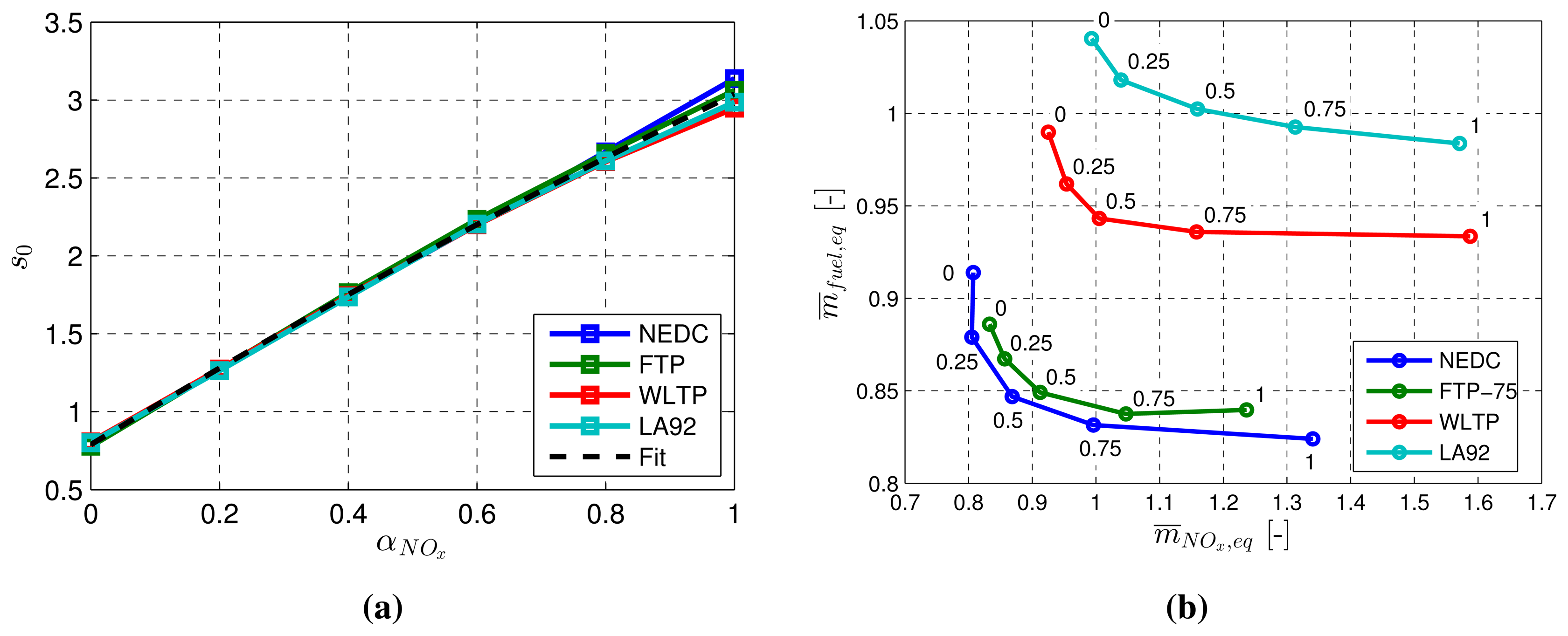
The goal of this section is to describe the methodology applied to identify the dependency of s₀ on α_NOx. The key idea is to apply an optimal control method to the optimization problem described by the Hamiltonian function in Equation (85), such as, for example, DP or PMP with constant values for the weighting factors, α_NOx and s₀. In this case, PMP is adopted, since it is more suitable for the present application of a forward-facing vehicle model, including many input and state variables. This procedure is applied for several different values of α_NOx, in order to identify, for each value, the corresponding unique constant equivalence factor, s₀, that ensures a charge sustaining condition.

The methodology is applied to various driving scenarios, in this case to the four well-known driving cycles, New European Driving Cycle (NEDC), Federal Test Procedure 75 (FTP-75), Worldwide Harmonized Light Vehicles Test Procedure (WLTP) and California Unified Cycle (LA92). The simulation results of the identification procedure are depicted in Figure 5a. The relationship between α_NOx and s₀ is almost linear. However, a linear fit can lead to s₀-values, which yield considerable deviations of the final SOC when simulating the vehicle on certain driving cycles without feedback. A quadratic fit, as indicated by the black dashed line, turned out to be more adequate for generating a unique relationship between the equivalence factors for the driving cycles considered.

Figure 5b shows the trade-off between fuel consumption and NO_x emissions, using charge-sustaining s₀-values for each α_NOx ∈ {0,0.25,0.5,0.75,1}. For each driving cycle, the corresponding curve represents the optimal trade-off for the approach presented using Equation (85). Any causal method based on Equation (85) cannot yield results that are to the left or below the corresponding trade-off for a specific driving cycle.

3.7. Controller Structure

Based on the mathematical derivation of the controller presented in the previous sections, the desired controller, to be tested in simulation and experimental tests in the following sections, is illustrated in Figure 6.

3.8. Calculation of SOC and m_NOx Reference Trajectories

The two PI controllers of Figure 6 require a proper definition of the reference trajectories for the respective controlled variables. The reference value for the SOC, ξ_ref(t), could simply be a constant value representing the desired final SOC, which also coincides with the initial value, ξ₀, to enforce a charge-sustaining constraint. Alternatively, the reference value can take into account that the current kinetic and potential energy of the vehicle can be recuperated in the future and stored as electrical energy with certain efficiencies, η_c,K, η_c,P, resulting in the following expression [48,49]:

$${\xi }_{\text{ref}}(t)={\xi }_0-\left({\eta }_{\text{c},\text{K}}\cdot \frac{\frac{1}{2}m(t)\cdot v^2(t)}{Q_0{V}_{\text{oc}}({\xi }_0)}+{\eta }_{\text{c},\text{P}}\cdot \frac{m(t)\cdot g\cdot (h(t)-h_0)}{Q_0{V}_{\text{oc}}({\xi }_0)}\right)$$

(86)

where h(t) − h₀ is the height difference between the current altitude and some reference altitude. The numerical values for η_c,K and η_c,P are both 0.65, which were obtained by manual tuning.

The reference cumulative emissions can be computed in a simple way by defining a specific emission level, m̄_NOx, Equation (27) expressed in units of mg/km:

$$m_{N{O}_x,\mathit{\text{ref}}}(t)={\int }_0^t{\overline{m}}_{N{O}_x}\cdot v(\tau )$$

(87)

The value for m̄_NOx can reflect a potential limit imposed by legislation. However, since the controller is purely causal, the controller cannot guarantee to keep the NO_x emissions below the limit. Therefore, a value for m_NOx should be chosen that is below the actual limit value issued, for example, by legislation.

Further, Equation (86) can easily be extended to account for the characteristics of plug-in HEVs. In this case, the constant, ξ₀, can be replaced by a driving distance-dependent reference trajectory, as proposed by the authors of [50]. Another possibility for both charge-sustaining and plug-in HEVs is to use predictive information to calculate a reference trajectory for the SOC [42,51], as well as for the NO_x emissions. Even further, predictive methods could be applied to directly optimize the Equations (32)–(35). However, the application of these ideas to the problem at hand is left for future research.

4. Results

First, an experimental validation of the models and of the methodology, as presented in Sections 2 and 3, is shown. Then, a case study is presented in which the benefit of using an RDE-ECMS compared to an ECMS with a constant emission-related equivalence factor, α_NOx, is analyzed.

4.1. Experimental Validation

The goal of this subsection is first to show that the RDE-ECMS presented in Section 3 works also in practice, and second, that the quasi-static modeling for the fuel consumption and the NO_x emissions is sufficient.

4.1.1. Experimental Setup

For the experimental validation of the RDE-ECMS, the method presented in Section 3 was applied both in simulation and in HIL experiments. In the HIL experiments, only the engine was used in real hardware. The longitudinal dynamics, as well as the vehicle components were simulated on a computer. This setup allowed for the measurement of the real fuel consumption and the real NO_x emissions without requiring the physical presence of the entire vehicle. For more details on HIL experiments, interested readers are referred to the literature [52–54].

In the HIL experiments here, the desired torque command, which is calculated by the energy management controller, is sent to the electronic control unit (ECU) of the engine, while the desired engine speed command is sent to the dynamometer of the engine test bench. The NO_x emissions are measured using a VDO/NGK UniNOx sensor manufactured by Continental AG, Hanover, Germany. This sensor is likely to be employed also in real vehicles, due its low price and due to its ability to additionally measure the air-to-fuel ratio. The fuel consumption is taken by the ECU-internal estimation.

4.1.2. Experimental Results on the WLTP

We used the following setup to compare the simulation results to the results obtained with the HIL experiments:

• driving cycle: WLTP (Class 3 Cycle);

• NO_x reference signal: as presented in Equation (87) with m̄_NOx = 1;

• SOC reference signal: 60% plus a correction as shown in Equation (86);

• initial condition for the emission-specific equivalence factor α_NOx(0) = 0;

• controller parameters k_p,ξ = 2, T_i,ξ = 480, p = 1, k_p,_NOx = 0.1, T_i,_NOx = 75,000, q = 1, for which the values were obtained by an appropriate optimization explained in the simulation case study in Section 4.2.

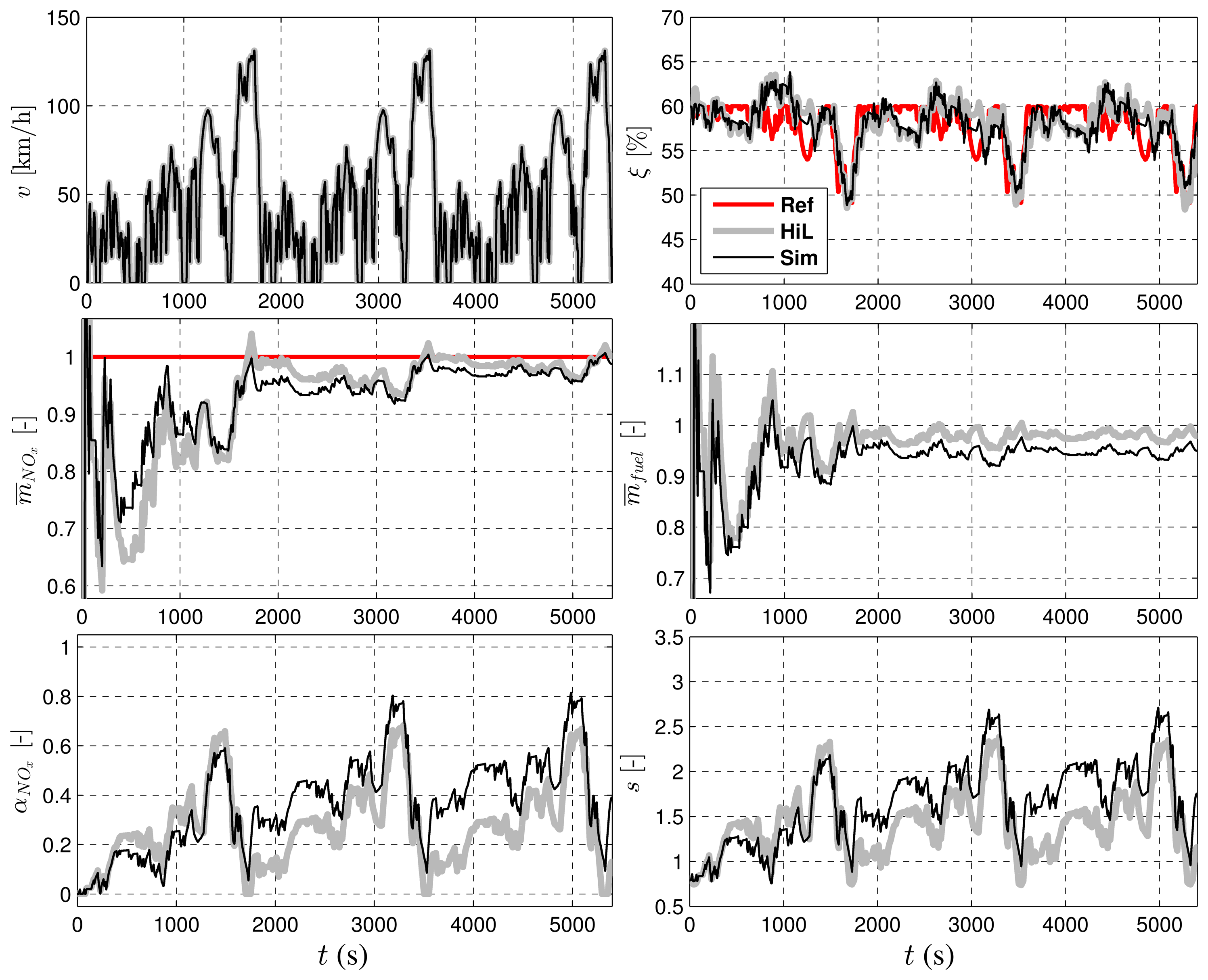
Figure 7 shows the vehicle speed, the battery SOC, the normalized specific NO_x emissions, the normalized specific fuel consumption and the equivalence factors, α_NOx and s, for both the NO_x emission and the battery power.

4.1.3. Comparison of the Simulation Results to the HIL Experiments

As can be seen from the figure, the vehicle speed trajectories of the simulation results and the HIL results are identical. The SOC trajectories of the simulation and the HIL results are similar; both are charge-sustaining at around the same SOC reference level. Furthermore, the NO_x trajectories of both are very similar; after an initial transient phase, the trajectories become more stable, and they approach the desired reference level. A similar behavior is observed for the specific fuel consumption that, in addition, exhibits a visible offset that is explained below. Further, the dynamics of the equivalence factor, α_NOx, are also similar for both the simulation and the HIL experiment. They both start from a value of zero and converge towards a value of one until the specific NO_x emissions approach the reference level. Due to the highway part, which requires the engine to be used a lot, the equivalence factor, α_NOx, is reduced to save NO_x emissions. In the subsequent city driving part, α_NOx again approaches a value of one until the next highway part, where the value of α_NOx is reduced once more. Furthermore, the trajectories for the equivalence factor, s, are close to each other. The preliminary conclusion from the comparison of the simulation results to the experimental results is that in practice, the RDE-ECMS works the same as in the simulation.

However, as can be seen from the figure, the RDE-ECMS cannot guarantee maintaining the NO_x emissions below the reference level since: (i) the strategy is purely causal; and (ii) the reference level can be too low for the controller to have a sufficient influence on the control action. Therefore, the reference trajectory has to be designed carefully.

The offset of the trajectories of the simulation and the HIL results is a consequence of some of the neglected dynamics in the engine model of the simulation. For example, the thermal dynamics are not considered in the simulation, although in practice, they can have an influence on the formation of pollutant emissions. In fact, such effects influence the behavior of the SOC and the NO_x control, such that the trajectories of the SOC, NO_x emissions, etc., become different for the results obtained with the simulation and the experiment. However, the offset between the trajectories is not a direct measure to quantify the modeling errors, because the trajectories show the actual, “uncorrected” emissions and the actual, “uncorrected” fuel consumption. For example, an offset of 5% in the trajectories for the fuel consumption does not mean that the true fuel consumption is 5% different, since there is also a certain offset in the SOC trajectories. Typically, a higher SOC means a also higher fuel consumption and also higher NO_x emissions. For a fair comparison, the equivalent NO_x emissions and the equivalent fuel consumption have to be calculated.

To make a fair comparison between the simulation and the experimental results, the NO_x emissions and the fuel consumption have to be corrected to take into account the different levels of the SOC. Here, the correction is made based on the following equations:

• m̄_fuel,eq denotes the distance specific, battery charge equivalent fuel consumption:

  $${\overline{m}}_{\text{fuel},\text{eq}}=\frac{1}{{\overline{m}}_{\text{fuel},\text{norm}}}\cdot \frac{\left({\int }_0^T{\stackrel{*}{m}}_{\text{fuel}}(t)dt+\mathrm{\Delta }{m}_{\text{fuel},\text{eq}}\right)}{{\int }_0^{T}v(t)dt}$$

  (88)
  where m̄_fuel,norm stands for a normalization value;

• m̄_NOx,eq denotes the distance specific, battery charge equivalent NO_x emissions:

  $${\overline{m}}_{N{O}_x,\text{eq}}=\frac{1}{{\overline{m}}_{N{O}_x,\text{norm}}}\cdot \frac{\left({\int }_0^T{\stackrel{*}{m}}_{N{O}_x}(t)dt+\mathrm{\Delta }{m}_{N{O}_x,\text{eq}}\right)}{{\int }_0^{T}v(t)dt}$$

  (89)
  where m̄_NOx,norm stands for a normalization value;

• Δm_fuel,eq and Δm_NOx,eq are the equivalent fuel mass and the equivalent NO_x mass as a function of the final battery charge, respectively [34]:

  $$\mathrm{\Delta }{m}_{\text{fuel},\text{eq}}=\{\begin{array}{ll}\frac{\mathrm{\Delta }{E}_{\text{b}}}{H_l}\cdot \frac{1}{{\overline{\eta }}_{\text{b}}^{(d)}\cdot {\overline{\eta }}_{\text{m}}^{(d)}\cdot {\overline{\eta }}_{\text{e}}}\hfill & \text{if}\mathrm{\Delta }{E}_{\text{b}}\ge 0\hfill \\ \frac{\mathrm{\Delta }{E}_b}{H_l}\cdot \frac{{\overline{\eta }}_b^{(c)}\cdot {\overline{\eta }}_m^{(c)}\cdot }{{\overline{\eta }}_e}\hfill & \text{if}\mathrm{\Delta }{E}_{\text{b}}<0\hfill \end{array}$$

  (90)
  $$\mathrm{\Delta }{m}_{N{O}_x,\text{eq}}=\frac{{\int }_0^T{\stackrel{*}{m}}_{N{O}_x}(t)dt}{{\int }_0^T{\stackrel{*}{m}}_{\mathit{\text{fuel}}}(t)dt}\cdot \mathrm{\Delta }{m}_{f,\text{eq}}$$

  (91)
  with η̄_b, η̄_m, η̄_e denoting the averaged efficiencies of the battery, the motor and the engine, while the superscript, ^(c) denotes “charging phase” and ^(d) denotes “discharging phase”.

• ΔE_b is the amount of net energy stored in the battery at the end of the driving cycle:

  $$\mathrm{\Delta }{E}_{\text{b}}=Q_0{\int }_{\xi (0)}^{\xi (T)}{V}_{\text{oc}}(\tilde{\xi })d\tilde{\xi }$$

  (92)

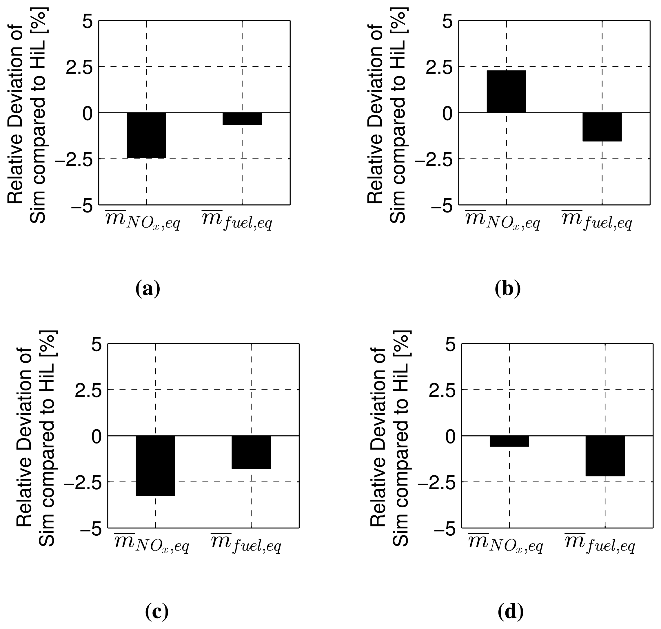
Figure 8 shows a comparison of the SOC-corrected equivalent NO_x emissions and corrected specific fuel consumption on the two driving cycles, NEDC and WLTP, for each, considering the two cases of a constant α_NOx and a variable α_NOx. The case with the constant α_NOx-value refers to a simulation without feedback control of the NO_x emissions. Instead, a constant α_NOx = 0 is used throughout the simulation. By contrast, the case with a variable α_NOx represents the case of the RDE-ECMS.

According to the figure, the results obtained with the simulation underestimate the results obtained with the HIL experiments. The error in all the simulations compared to the experimental data is well below 5%. Therefore, quasi-static models for the fuel consumption and the NO_x emissions can be considered to be accurate enough for the simulation on the NEDC and WLTP driving cycles.

4.2. Simulation Case Study

By now, it was shown that the RDE-ECMS can simultaneously control the SOC and the NO_x emissions. To show in addition that the RDE-ECMS yields a lower fuel consumption than a non-adaptive ECMS, these two strategies are compared on four different driving cycles, namely the NEDC, the FTP-75, the WLTP and the LA92.

Assume that the RDE have to be lower than a specific value, say 1.02 or 102% for the specific NO_x emissions in this case. Two causal strategies are considered, which respect this NO_x limit: (1) a non-adaptive PI-controlled ECMS, which is the RDE-ECMS, but with a fixed value for α_NOx; and (2) the RDE-ECMS presented in Section 3 with a specific NO_x reference value of 1.0.

The non-adaptive ECMS was tuned to respect the NO_x emission limit on the worst case driving cycle, which, here, is LA92, while giving the lowest possible fuel consumption on all driving cycles. The optimized parameters of the non-adaptive PI-controlled ECMS are k_p,ξ = 2, T_i,ξ = 480, p = 1 and α_NOx = 0. For comparison, the parameters of the RDE-ECMS are k_p,ξ = 2, T_i,ξ = 480, k_p,_NOx = 0.1, T_i,NOx = 75,000, q = 1 and α_NOx(0) = 0. Note that, for simplicity, the values for the parameters, k_p,ξ and T_i,_ξ, of the RDE-ECMS were taken from the non-adaptive ECMS. The two other parameters, k_p,NOx and T_i,NOx, were optimized on the NEDC and the WLTP driving cycles to yield an acceptable reference tracking, namely neither a too fast nor a too slow tracking. To ensure a fair comparison, the initial value for α_NOx was chosen to be equal to that of the non-adaptive ECMS.

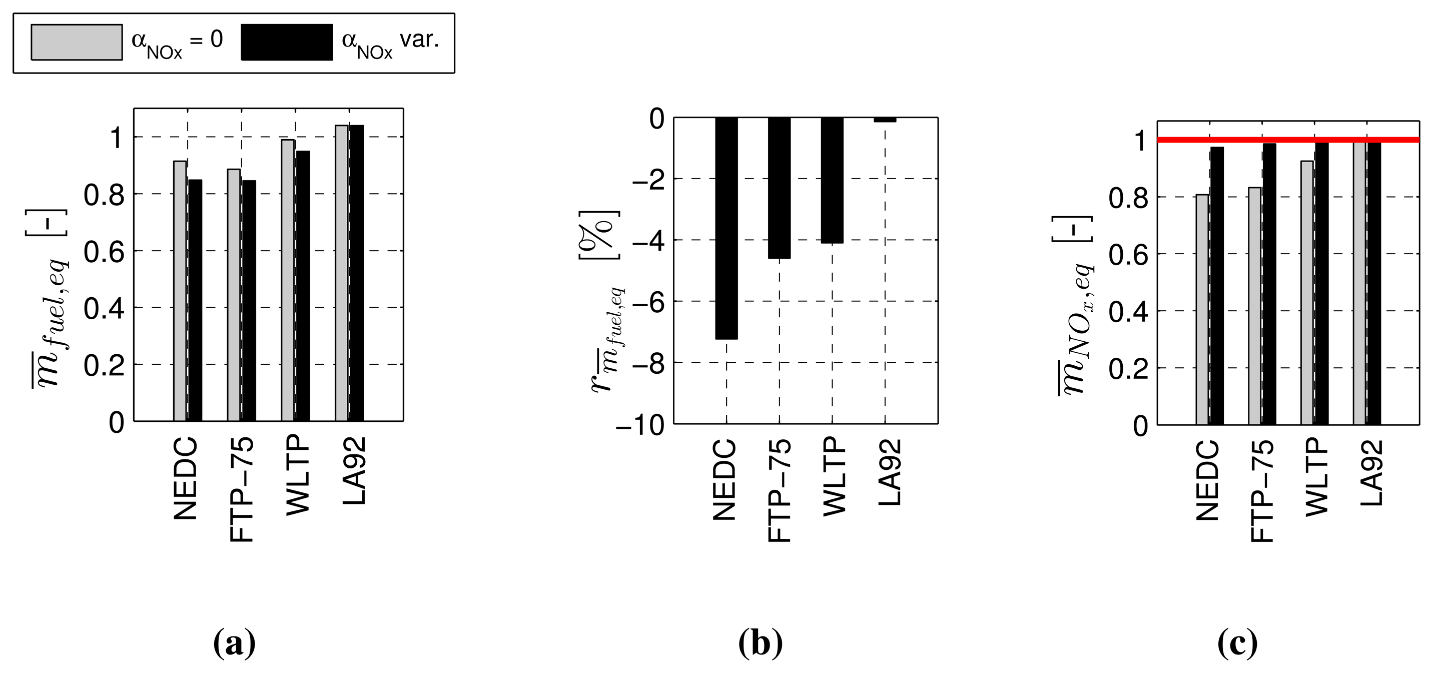
These two strategies were applied on each of five repetitions of the four different driving cycles, NEDC, FTP-75, WLTP and LA92. Figure 9 shows the normalized specific equivalent fuel consumption, the relative fuel consumption difference of the RDE-ECMS compared to the non-adaptive ECMS and the normalized specific equivalent NO_x emissions for both the non-adaptive ECMS (“α_NOx = 0”) and the RDE-ECMS (“α_NOx var.”, where “var.” stands for “variable” in the meaning of “not fixed”).

As seen from Figure 9b, the fuel savings of the RDE-ECMS amount to 0%–7% compared to the non-adaptive ECMS. On all driving cycles, both strategies respect the NO_x emission limit, indicated as a red line in the plot on the right-hand side. In the case of the LA92 driving cycle, the RDE-ECMS behaves the same as the non-adaptive ECMS, which is the reason that there are practically no fuel savings. On all other driving cycles, the RDE-ECMS provides a lower fuel consumption than the non-adaptive ECMS, since the RDE-ECMS increases the emission-related equivalence factor, α_NOx, to move along the optimal NO_x-fuel trade-off.

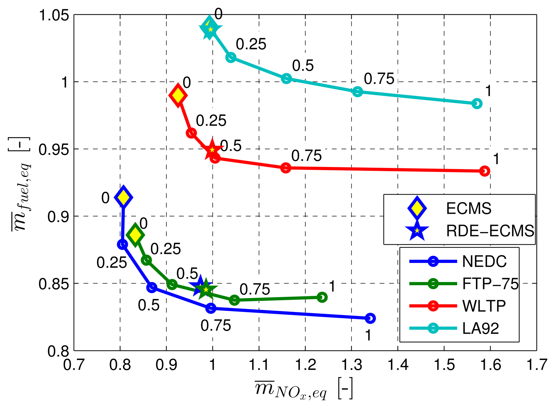
Figure 10 shows the performance of the RDE-ECMS and the non-adaptive ECMS in relation to the optimal trade-off between the fuel consumption and NO_x emissions already shown in Figure 5b. The non-adaptive ECMS (“diamond marker”) achieves practically identical performance as the optimal non-causal solution for α_NOx = 0 in terms of fuel consumption and NO_x emissions. The RDE-ECMS (“star marker”) achieves a performance close to the optimal trade-off curve for the driving cycles, FTP-75, WLTP and LA92. For the NEDC, there is still a potential to reduce the fuel consumption by about 1.6% for the same amount of NO_x emissions as calculated with the non-causal ECMS.

Overall, the RDE-ECMS proved to minimize the fuel consumption, while tracking a reference NO_x emission level and sustaining the battery charge.

5. Conclusions

This paper presents an energy management strategy to account for NO_x RDE of a diesel HEV. The method is based on the ECMS, which is extended with a state accounting for the NO_x emissions. As demonstrated in simulation, as well as in HIL experiments, the strategy is able to minimize the fuel consumption, while following given reference trajectories for the NO_x emissions and the battery SOC. By simulation, the strategy is shown to optimally adjust the trade-off between the fuel consumption and NO_x emissions during operation. Compared to a conservative non-adaptive strategy, the advantages in terms of fuel consumption amount to more than 7% in favor of the proposed method. The strategy can be employed also in plug-in HEVs, without the need of adjusting the controller structure, by only modifying the reference trajectory for the battery SOC.

So far, the presented RDE-ECMS has been applied to warm engine conditions. A future evolution of this strategy will be to investigate the control of tailpipe NO_x emissions for a diesel HEV equipped with a SCR system. This will require a model of the reduction efficiency of the aftertreatment system as a function of an additional state, represented by the thermal state of the SCR system. Moreover, a further potential is seen in the optimal design of the reference trajectories for the SOC and the NO_x emissions.

References

- Rubino, L.; Bonnel, P.; Hummel, R.; Krasenbrink, A.; Manfredi, U.; de Santi, G.; Perotti, M.; Bomba, G. PEMS Light Duty Vehicles Application: Experiences in downtown Milan. In Proceedings of the 8th International Conference on Engines for Automobiles, Capri, Italy, 16–20 September 2007.
- Vojtisek-Lom, M.; Fenkl, M.; Dufek, M.; Mareš, J. Off-Cycle, Real-World Emissions of Modern Light Duty Diesel Vehicles. Proceedings of the 9th International Conference on Engines and Vehicles, Capri, Italy, 13–18 September 2009.
- Rubino, L.; Bonnel, P.; Hummel, R.; Krasenbrink, A.; Manfredi, U.; Santi, G.D. On-road emissions and fuel economy of light duty vehicles using PEMS: Chase-testing experiment. SAE Int. J. Fuels Lubr. 2009, 1, 1454–1468. [Google Scholar]
- Weiss, M.; Bonnel, P.; Hummel, R.; Provenza, A.; Manfredi, U. On-road emissions of light-duty vehicles in Europe. Environ. Sci. Technol. 2011, 45, 8575–8581. [Google Scholar]
- Weiss, M.; Bonnel, P.; Hummel, R.; Steininger, N. A Complementary Emissions Test for Light-Duty Vehicles: Assessing the Technical Feasibility of Candidate Procedures; European Commission, Joint Research Centre: Ispra, Italy, 2013. [Google Scholar]
- Johnson, V.H.; Wipke, K.B.; Rausen, D.J. HEV Control Strategy for Real-Time Optimization of Fuel Economy and Emissions. Proceedings of the Future Car Congress, Arlington, VA, USA, 2–6 April 2000.
- Paganelli, G.; Tateno, M.; Brahma, A.; Rizzoni, G.; Guezennec, Y.; Transportation, I. Control Development for a Hybrid-Electric Sport-Utility Vehicle: Strategy, Implementation and Field Test Results. Proceedings of the IEEE American Control Conference, Arlington, VA, USA, 25–27 June 2001; Volume 6, pp. 5064–5069.
- Musardo, C.; Staccia, B.; Midlam-Mohler, S.; Guezennec, Y.; Rizzoni, G. Supervisory Control for NOx Reduction of an HEV with a Mixed-Mode HCCI/CIDI Engine. Proceedings of the IEEE American Control Conference (ACC), Portland, OR, USA, 8–10 June 2005; Volume 6, pp. 3877–3881.
- Sagha, H.; Farhangi, S.; Asaei, B. Modeling and Design of a NOx Emission Reduction Strategy for Lightweight Hybrid Electric Vehicles. Proceedings of the IECON'09. 35th Annual Conference of IEEE Industrial Electronics, Porto, Portugal, 3–5 November 2009; pp. 334–339.
- Millo, F.; Ferraro, C.V.; Rolando, L. Analysis of different control strategies for the simultaneous reduction of CO2 and NOx emissions of a diesel hybrid passenger car. Int. J. Veh. Des. 2012, 58, 427–448. [Google Scholar]
- Alipour, H.; Asaei, B. An online fuel consumption and emission reduction power management strategy for plug-in hybrid electric vehicles. Veh. Eng. 2013, 1, 41–55. [Google Scholar]
- Paganelli, G.; Guerra, T.M.; Delprat, S.; Santin, J.J.; Delhom, M.; Combes, E. Simulation and assessment of power control strategies for a parallel hybrid car. Proc. Instit. Mech. Eng. D J. Automob. Eng. 2000, 214, 705–717. [Google Scholar]
- Delprat, S.; Guerra, T.; Rimaux, J. Control Strategies for Hybrid Vehicles: Optimal Control. In Proceedings of the 56th IEEE Vehicular Technology Conference, VTC 2002-Fall, Vancouver, BC, Canada, 24–28 September 2002; Volume 3, pp. 1681–1685.
- Kessels, J.; Willems, F.; Schoot, W.; van den Bosch, P. Integrated Energy & Emission Management for Hybrid Electric Truck with SCR Aftertreatment. Proceedings of the IEEE Vehicle Power and Propulsion Conference, VPPC 2010, Lille, Belgium, 1–3 September 2010; pp. 1–6.
- Kum, D. Modeling and Optimal Control of Parallel HEVs and Plug-in HEVs for Multiple Objectives. Ph.D. Thesis, The University of Michigan, Ann Arbor, MI, USA, 2010. [Google Scholar]
- Kum, D.; Peng, H.; Bucknor, N.K. Supervisory control of parallel hybrid electric vehicles for fuel and emission reduction. J. Dyn. Syst. Meas. Control 2011, 133. [Google Scholar] [CrossRef]
- Ao, G.Q.; Qiang, J.X.; Zhong, H.; Mao, X.J.; Yang, L.; Zhuo, B. Fuel economy and NOx emission potential investigation and trade-off of a hybrid electric vehicle based on dynamic programming. Proc. Inst. Mech. Eng. D J. Automob 2008, 222, 1851–1864. [Google Scholar]
- Serrao, L.; Sciarretta, A.; Grondin, O.; Chasse, A.; Creff, Y.; di Domenico, D.; Pognant-Gros, P.; Querel, C.; Thibault, L. Open issues in supervisory control of hybrid electric vehicles: A unified approach using optimal control methods. Oil Gas Sci. Technol. Rev. IFP Energies Nouv. 2013, 68, 23–33. [Google Scholar]
- Sezer, V.; Gokasan, M.; Bogosyan, S. A novel ECMS and combined cost map approach for high-efficiency series hybrid electric vehicles. IEEE Trans. Veh. Technol. 2011, 60, 3557–3570. [Google Scholar]
- Grondin, O.; Thibault, L.; Moulin, P.; Chasse, A.; Sciarretta, A. Energy Management Strategy for Diesel Hybrid Electric Vehicle. In Proceedings of the 2011 IEEE Vehicle Power and Propulsion Conference (VPPC), Chicago, IL, USA, 6–9 September 2011; pp. 1–8.
- Nüesch, T.; Wang, M.; Isenegger, P.; Onder, C.H.; Steiner, R.; Macri-Lassus, P.; Guzzella, L. Optimal energy management for a diesel hybrid electric vehicle considering transient PM and quasi-static NOx emissions. Control Eng. Pract. 2014. [Google Scholar] [CrossRef]
- Predelli, O.; Bunar, F.; Manns, J.; Buchwald, R.; Sommer, A. Laying out Diesel-Engine Control Systems in Hybrid Drives Hybrid Vehicles and Energy Management. In Hybrid Vehicles and Energy Management; ITS Niedersachsen: Braunschweig, Germany, 2007. [Google Scholar]
- Lindenkamp, N.; Stöber-Schmidt, C.P.; Eilts, P. Strategies for Reducing NOx- and Particulate Matter Emissions in Diesel Hybrid Electric Vehicles. Proceedings of the SAE World Congress & Exhibition, Detroit, MI, USA, 20–23 April 2009.
- Johri, R.; Salvi, A.; Filipi, Z. Optimal Energy Management for a Hybrid Vehicle using Neuro-Dynamic Programming to Consider Transient Engine Operation. Proceedings of the ASME 2011 Dynamic Systems and Control Conference and Bath/ASME Symposium on Fluid Power and Motion Control, Arlington, VA, USA, 31 October–2 November 2011; Volume 2, pp. 279–286.
- Wang, Y.; Zhang, H.; Sun, Z. Optimal control of the transient emissions and the fuel efficiency of a diesel hybrid electric vehicle. Proc. Inst. Mech. Eng. D J. Automob. Eng. 2013, 227, 1546–1561. [Google Scholar]
- Grondin, O.; Quérel, C. Transient torque control of a diesel hybrid powertrain for NOx limitation. Engine Powertrain Control Simul. Model 2012, 3, 286–295. [Google Scholar]
- Guzzella, L.; Sciarretta, A. Vehicle Propulsion Systems, 3rd ed.; Springer-Verlag: Berlin, Germany, 2013. [Google Scholar]
- Park, D.; Seo, T.; Lim, D.; Cho, H. Theoretical Investigation on Automatic Transmission Efficiency. In Proceedings of the International Congress & Exposition, Detroit, MI, USA, 26–29 February 1996.
- Shankar, R.; Marco, J.; Assadian, F. The novel application of optimization and charge blended energy management control for component downsizing within a plug-in hybrid electric vehicle. Energies 2012, 5, 4892–4923. [Google Scholar]
- Ebbesen, S.; Elbert, P.; Guzzella, L. Engine downsizing and electric hybridization under consideration of cost and drivability. Oil Gas Sci. Technol. Rev. IFP Energies Nouv. 2012, 68, 109–116. [Google Scholar]
- Filipi, Z.; Fathy, H.; Hagena, J.; Knafl, A.; Ahlawat, R.; Liu, J.; Jung, D.; Assanis, D.; Peng, H.; Stein, J.L. Engine-in-the-Loop Testing for Evaluating Hybrid Propulsion Concepts and Transient Emissions-HMMWV Case Study. In Proceedings of the SAE 2006 World Congress & Exhibition, Detroit, MI, USA, 3–6 April 2006.
- Nanophosphate High Power Lithium Ion Cell ANR26650M1-B. In MD100113-01 Data Sheet; A123 Systems, Inc: Waltham, MA, USA, 2011.
- Lee, J.; Yi, J.; Shin, C.; Yu, S.; Cho, W. Modeling the effects of the cathode composition of a lithium iron phosphate battery on the discharge behavior. Energies 2013, 6, 5597–5608. [Google Scholar]
- Sciarretta, A.; Guzzella, L. Control of hybrid electric vehicles. IEEE Control Syst. Mag. 2007, 27, 60–70. [Google Scholar]
- Kim, N.; Cha, S.; Peng, H. Optimal control of hybrid electric vehicles based on pontryagin's minimum principle. IEEE Trans. Control Syst. Technol. 2011, 19, 1279–1287. [Google Scholar]
- Murgovski, N.; Johannesson, L.; Sjöberg, J.; Egardt, B. Component sizing of a plug-in hybrid electric powertrain via convex optimization. Mechatronics 2012, 22, 106–120. [Google Scholar]
- Kothare, M.V.; Campo, P.J.; Morari, M.; Nett, C.N. A unified framework for the study of anti-windup designs. Automatica 1994, 30, 1869–1883. [Google Scholar]
- Geering, H.P. Optimal Control with Engineering Applications; Springer-Verlag: Berlin, Germany, 2007. [Google Scholar]
- Bertsekas, D.P. Dynamic Programming and Optimal Control; Athena Scientific: Nashua, NH, USA, 2005; Volume 3. [Google Scholar]
- Zentner, S.; Asprion, J.; Onder, C.; Guzzella, L. An equivalent emission minimization strategy for causal optimal control of diesel engines. Energies 2014, 7, 1230–1250. [Google Scholar]
- Ambühl, D. Energy Management Strategies for Hybrid Electric Vehicles. Ph.D. Thesis, ETH Zurich, Zurich, Switzerland, 2009. [Google Scholar]
- Ambühl, D.; Guzzella, L. Predictive reference signal generator for hybrid electric vehicles. IEEE Trans. Veh. Technol. 2009, 58, 4730–4740. [Google Scholar]
- Koot, M.; Kessels, J.; de Jager, B.; Heemels, W.; van den Bosch, P.P.; Steinbuch, M. Energy management strategies for vehicular electric power systems. IEEE Trans. Veh. Technol. 2005, 54, 771–782. [Google Scholar]
- Ambühl, D.; Sundström, O.; Sciarretta, A.; Guzzella, L. Explicit optimal control policy and its practical application for hybrid electric powertrains. Control Eng. Pract. 2010, 18, 1429–1439. [Google Scholar]
- Sciarretta, A.; Back, M.; Guzzella, L. Optimal control of parallel hybrid electric vehicles. IEEE Trans. Control Syst. Technol. 2004, 12, 352–363. [Google Scholar]
- Opila, D.F.; Wang, X.; McGee, R.; Gillespie, R.B.; Cook, J.A.; Grizzle, J.W. An energy management controller to optimally trade off fuel economy and drivability for hybrid vehicles. IEEE Trans. Control Syst. Technol. 2012, 20, 1490–1505. [Google Scholar]
- Kutter, S. Eine Prädiktive und Optimierungsbasierte Betriebsstrategie für Autarke und Extern Nachladbare Hybridfahrzeuge. Ph.D. Thesis, Dresden University of Technology, Dresden, Germany, 2013; In German. [Google Scholar]
- Keulen, T.V.; Jager, B.D.; Steinbuch, M. An Adaptive Sub-Optimal Energy Management Strategy for Hybrid Drive-Trains. In Proceedings of the 17th International Federation of Automatic Control (IFAC) World Congress, Seoul, Korea, 6–11 July 2008; pp. 102–107.
- Keulen, T.V.; Mullem, D.V.; Jager, B.D.; Kessels, J.T.; Steinbuch, M. Design, implementation, and experimental validation of optimal power split control for hybrid electric trucks. Control Eng. Pract. 2012, 20, 547–558. [Google Scholar]
- Tulpule, P.; Stockar, S.; Marano, V.; Rizzoni, G. Optimality Assessment of Equivalent Consumption Minimization Strategy for PHEV Applications. Proceedings of the ASME Dynamic Systems and Control Conference (DSCC), Hollywood, CA, USA, 12–14 October 2009; Volume 2, pp. 265–272.
- Kutter, S.; Bäker, B. Predictive Online Control for Hybrids: Resolving the Conflict between Global Optimality, Robustness and Real-Time Capability. Proceedings of the 2010 IEEE Vehicle Power and Propulsion Conference (VPPC), Lille, France, 1–3 September 2010; pp. 1–7.
- Shafai, E. Fahrzeugemulation an einem Dynamischen Verbrennungsmotor-Prüfstand. Ph.D. Thesis, ETH Zurich, Zurich, Switzerland, 1990; In German. [Google Scholar]
- Chasse, A.; Sciarretta, A. Supervisory control of hybrid powertrains: An experimental benchmark of offline optimization and online energy management. Control Eng. Pract. 2011, 19, 1253–1265. [Google Scholar]
- Ott, T.; Onder, C.; Guzzella, L. Hybrid-electric vehicle with natural gas-diesel engine. Energies 2013, 6, 3571–3592. [Google Scholar]