The assessment of exposure to traffic and industry related pollution continues to be a challenge. Most epidemiological studies that assess health effects of pollution use fixed monitoring sites and different modelling techniques (e.g., kriging, dispersion), but adequate information and data are not always available [1]. For example, kriging has been used both at the national and regional scale [2], but it has been criticised for its inability to capture air pollution at very short distances [3]. Other estimation techniques such as microenvironment monitoring have been hampered by high costs related to data collection especially when dealing with a large cohort [4,5]. Furthermore, the use of traditional dispersion models have been restricted because of their expensive data demands and lack of precision in the requisite meteorological or emissions data required for making accurate predictions [6,7].

Recently, land use regression (LUR) modelling has been proposed as an alternative approach to address some of the limitations by assessing the intra-urban spatial variability of ambient air pollutants in urban and industrial settings. LUR modelling captures localized variations in ambient air pollution more effectively and economically than some of the conventional approaches discussed above [2]. In addition, LUR modelling predicts ambient air pollution concentrations at given sites based on the surrounding land use, traffic, population and dwelling counts, and physical characteristics such as elevation [6]. Several researchers [2,6,8] have provided critical reviews of LUR studies and emphasized its potential role in estimating exposure to outdoor air pollution.

Annoyance caused by air pollution has been suggested as an indicator for ambient air pollution exposure [9,10]. This exposure estimation technique incorporates broader scopes and domains such as quality of life and community values [10,11]. Invariably, there are contrasting reports showing the relationship between annoyance scores and modelled ambient exposures. For example, while examining the predictors of perceived annoyance from air pollution in six European cities (Athens, Basel, Milan, Oxford, Prague, and Helsinki), Rotko et al. [12] found no association between outdoor nitrogen dioxide (NO₂) pollution levels and annoyance scores at individual levels. In Sweden, Forsberg et al. [13] reported no significant association between sulphur dioxide (SO₂) and annoyance scores. When comparing self-reported traffic intensity to modelled air pollution from traffic in three birth cohorts from three countries: the Netherlands; Germany; and Sweden, Heinrich et al. [14] found weak association between the subjective self-reported assessments of exposure and NO₂ modelled estimates. In addition, while examining the relationship between publicly available air quality data and public perception of air quality in London, UK, Williams and Bird [11] reported that perception of pollution exposure was not consistent with air quality data for urban and suburban areas although there were some trends with women and older people perceiving higher levels of air pollution than their female and younger counter parts.

On the other hand, while examining whether a questionnaire-based indicator (annoyance) of ambient air pollution can be a useful proxy for assessing the within-area variability of air quality in Switzerland, Oglesby et al. [15] reported a strong association between annoyance and modelled NO₂ concentration at home, but also found that smoking, workplace dust exposure, and respiratory symptoms were significant predictors of individual annoyance score. While Forsberg et al. [13] reported a lack of association between annoyance and SO₂, they did report a high correlation between NO₂ concentration and annoyance related to air pollution and traffic exhaust fumes. Furthermore, Jacquemin et al. [16] reported an association between self-reported annoyances caused by ambient air pollution and outdoor NO₂ concentration levels in 20 cities from 10 European countries. They concluded that annoyance scores could be a useful measure of perceived outdoor air quality. Smith et al. [17] found that the degree of concern voiced about foul air was closely related to the level of ambient air pollution experienced by their study subjects in Nashville, Tennessee. Similarly, Modig and Forsberg [18] reported a significant increase of people self-assessed annoyance with rising levels of modelled NO₂ concentrations in three Swedish cities (Umea, Uppsala, and Gothenburg). In Oslo, Norway, Piro et al. [9] found that annoyance to air pollution problems are strongly associated with increased levels of modelled air pollution concentrations

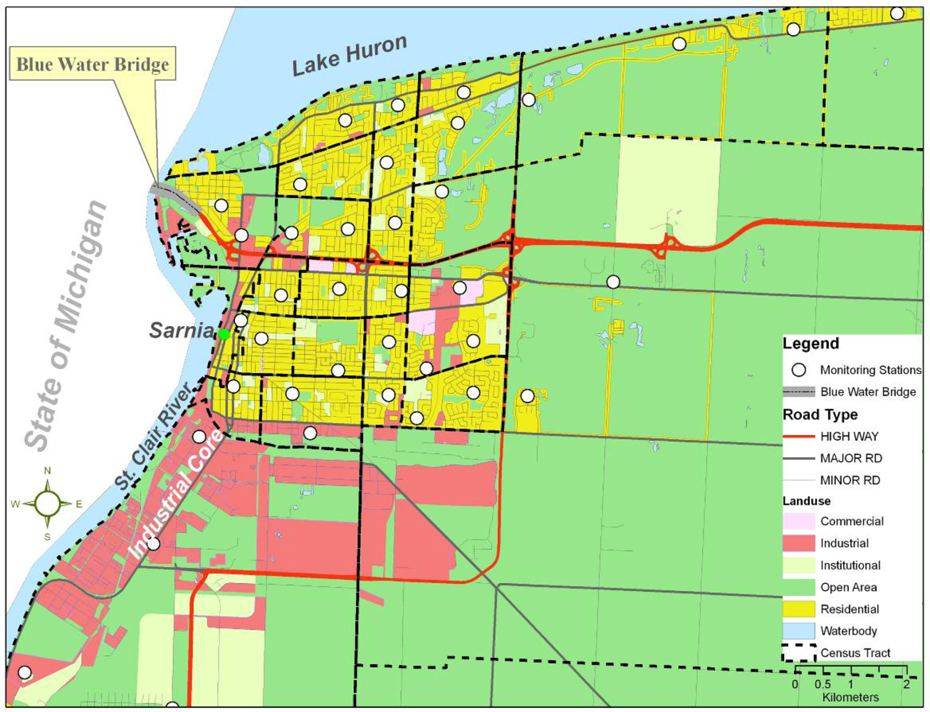
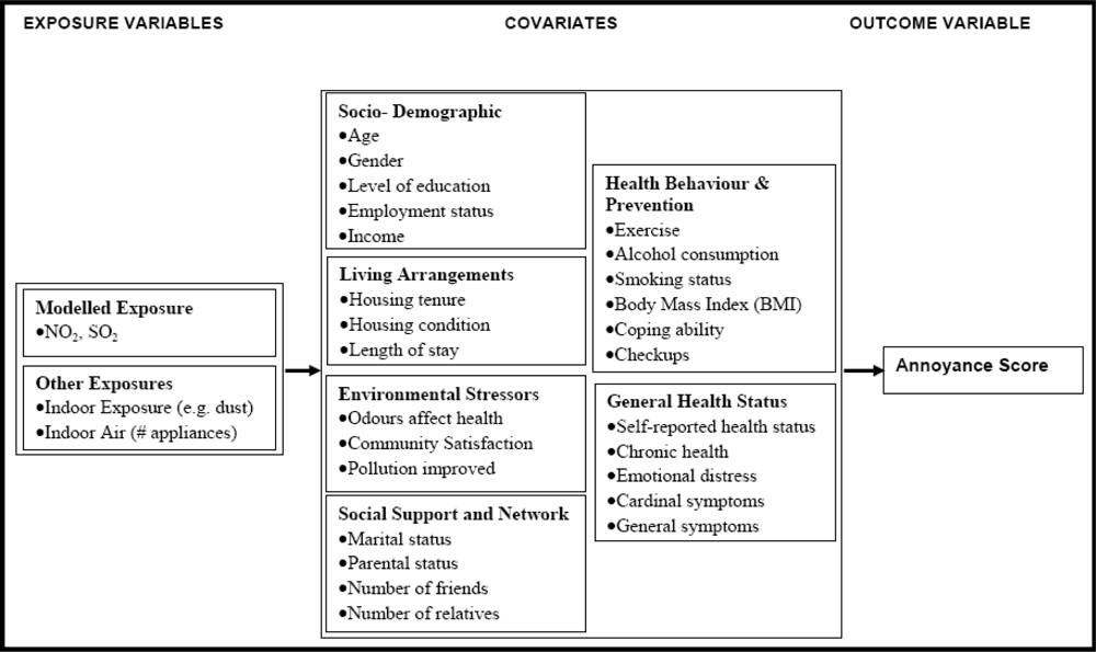
This study extends the emerging literature on the relationship between odour annoyance and air pollution in Sarnia “Chemical Valley”, Ontario (Canada), a sentinel high exposure environment; with the following specific objectives: a) to determine the correlations between odour annoyance score and modelled NO₂ and SO₂ at individual and census tract levels; b) to examine the individual determinants of odour annoyance caused by industrial pollution; and c) to establish exposure–response relationship between NO₂ and SO₂ exposure and odour annoyance.

This study is informed by risk perception and odour annoyance literature [19–21]. In general, health risk perception plays an important role on how individuals and the public respond to environmental exposures. While examining people's perceptions of problems and social cohesion in neighbourhoods in Quebec City, Quebec, Pampalon et al. [22] found that perceptions of place appear to be significant predictors of health and well-being. Likewise, in Glasgow, Ellaway et al. [23] reported that self-rated health is associated with perceived neighbourhood problems and cohesion. In Hamilton, Ontario, Elliott et al. [24] found that the relationships between environmental exposure and health outcomes are mediated by risk perception of exposure (e.g., air pollution); and that they cannot be divorced from the wider community context in which they occur. However, there are observed discrepancies between lay persons’ perception of environmental and technological risks and those of the scientific and policy experts on the difference between “reality” and perception [19]. These differences have raised concern and even perplexity among those responsible for the management of environment risk.

Scientists assume they have more objective understanding of risk due to their rigorous experimental studies, epidemiological surveys, and probabilistic risk analysis; but the lay persons’ understanding of risk is based on misperceptions or misunderstandings of the objective (real) risk [19]. However, some studies have reported that lay people are not ignorant of what is real risk but (when compared to experts) lay persons employ a broader and richer kind of rationality influenced by complex social, political, and cultural processes to assess exposure to environmental risk [19]. Lay persons take into consideration qualitative issues such as future generation and their personal lives, and bring in their beliefs and values to judge the “reality” of environmental risk [21]. Hence, lay persons’ perception of air pollution might be real because they depend in part on the pollution concentrations levels they are exposed to. Consequently, self-reported annoyance may correlate with monitored or modelled exposure. Thus, public concerns could not be blamed on ignorance or irrationality but rather to the sensitivity to technical, social, and psychosocial qualities of hazards that are not well-modelled in technical risk assessment [21].

Odours from industrial sources, such as the petrochemical plants in Sarnia, have been shown to considerably impact general health and well-being by affecting both the physiological and psychosocial status of people [20,25]. Such impacts are reinforced when air pollution odours are absorbed by building materials and then released slowly overtime [26,27]. Shusterman et al. [20] argued that odours appear to contribute to lay people’s judgment of environmental air quality, and provide important diagnostic information in appraising the potential threats to health and well-being. As a result, perceptual ideas about toxicity of environmental pollution seem to suggest that “if environments smell bad, they’re probably damaging to health” [28, p. 412] or at the very least, they might cause annoyance – feelings of displeasure associated with agents or conditions believed to have adverse effects on an individual or groups of individuals. Neutra et al. [29] identified odour annoyance as a powerful effect modifier in several studies of symptom rates around hazardous waste sites which can be extended to a highly exposed environment such as Sarnia because of the numerous petrochemical industries in the region. Annoyance responses are modified by personal factors and community level factors, such as age, gender and perceived health status [9,26,30], attitudes toward the exposure source, and individual sociodemographic characteristics [13,26]. For example, Forsberg et al. found that the frequency of reporting annoyance was high among women and people with respiratory illnesses like asthma. These discussions above provide a background for interpreting the relationship between modelled pollution and annoyance, and the determinants of annoyance within the context of a highly exposed environment.

The mean LUR modelled pollution concentrations for individuals (N = 774) was 13.82 ± 1.64 ppb for NO₂ and 3.17 ± 1.53 ppb for SO₂. The 24 hour ambient air quality criteria (AAQC) developed by the Ontario Ministry of Environment [42] for NO₂ and SO₂ concentrations was “100 ppb”. The correlation coefficients between modelled NO₂ and SO₂ were 0.49 and 0.65 at individual and census tract levels, respectively. Overall, 34% of respondents reported no annoyance at all; 50% reported little annoyance (1–7); and 16% reported high annoyance (≥8). The overall mean annoyance was 3.22 with a median of 2. Table 1 shows the distribution of annoyance scores by modelled pollutants and gender.

The results show that annoyance scores increase with increasing NO₂ and SO₂ pollution concentrations. Female respondents reported comparatively higher mean annoyance scores than their male counter parts. The results also showed a wide range of perception at a given level of ambient air pollution based on age group (Table 2). When the mean annoyance scores were compared, age groups showed a trend with older people less annoyed than the younger ones with the exception for the 18–24 group. In general, the mean annoyance score corresponded to the gradient of the modelled pollutants despite age differences.

The Pearson correlation coefficients between odour annoyance and modelled pollutants were all positive and significant but low for NO₂ (r = 0.15) and SO₂ (r = 0.13) at the individual level compared to the high coefficients of 0.56 and 0.67 at the census tract level for NO₂ and SO₂, respectively (Table 3). The univariate linear regression analyses indicate that modelled NO₂ and SO₂ concentrations each explained only 2% of the annoyance scores variance at the individual level but 32 and 44% of the variances at the census tract level, respectively (Table 4).

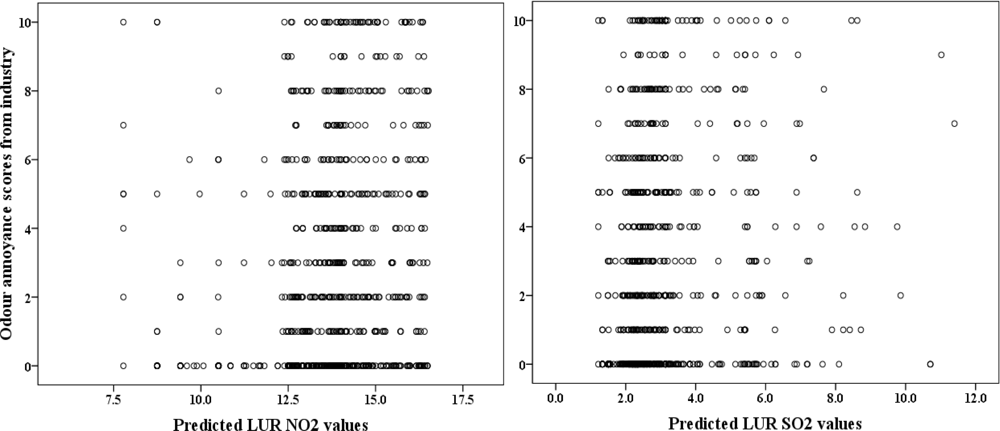
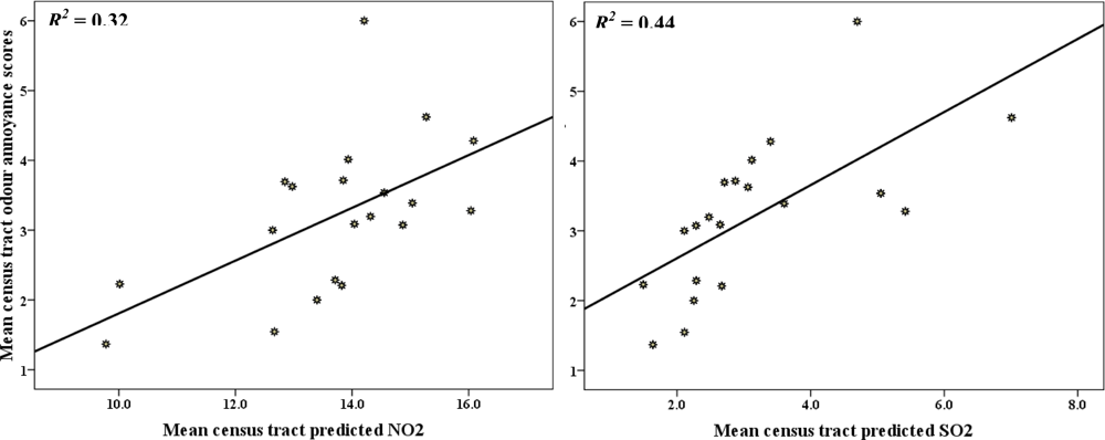
Figure 3 shows the scatterplot between modelled pollutant concentrations and annoyance scores observed at an individual level; while Figure 4 shows the distribution and lines of best fit between mean census tract odour annoyance scores and modelled NO₂ and SO₂ concentrations. The results show that annoyance score is better predicted at the census tract than the individual level.

In the multivariate logistic regression analysis, each possible determinant was evaluated one at a time, and a dichotomized odour annoyance rating (annoyance score ≥ 8 versus < 8) of industrial odour disturbances was used as an outcome variable. We examined the influence of modelled NO₂ and SO₂ on annoyance reporting separately. Table 5 shows the relationship between high annoyance and modelled NO₂ concentrations and also together with other covariates. When age and gender were controlled (Model II, Table 5), the 3^rd and 4^th high NO₂ quartiles retained significant influence on high odour annoyance reporting. Age did not show any significance influence on high annoyance reporting but age groups reflected annoyance score gradient with older people reporting less likelihood of high annoyance score. Gender was significant with females more likelihood to report high annoyance than their male counter parts (OR = 2.17, p-value < 0.001). In model III, the introduction of occupational exposure to dust made significant effect on odour annoyance score reporting with those more exposed at work more likely to report odour annoyance (OR = 1.57, p-value < 0.05). When sociodemographic variables, general health status (i.e. health status, cardinal symptoms), and perception of odours were controlled (Model IV), the odd ratios of reporting high odour annoyance increased for people exposed to high NO₂ pollution quartiles. Residents exposed to the 3^rd and 4^th NO₂ concentrations quartiles were more than 3 times more likely to report high annoyance than residents who are exposed to the 1^st and 2^nd pollution concentrations quartiles. In the final model (Model V, Table 5), high pollution concentration, gender, odour perception (that odours impact health and have not improved in the last 5 years), and the ability to cope with day-to-day demands showed significant influence on reporting of high odour annoyance. The multivariate modelling suggests that the relationship between odour annoyance and NO₂ concentrations was influenced by gender, cardinal symptoms, and odour perception. The inabilities to cope with day-to-day demands also influence high odour annoyance reporting (OR = 2.06, p-value < 0.05). With the first order interaction, the final NO₂-based model showed an improved model with acceptable goodness of fit (ρ²) of 0.21 [43]. The goodness of fit is defined as one minus the ratio of the maximum log likelihood values of the fitted and constant only-term (null) models. Calculated values for goodness of fit range from zero to one, and values between 0.2 and 0.4 represent a very good fit of the model [43].

The relationship between modelled SO₂ concentrations and high odour annoyance scores remained significant even after we controlled for age and gender (Model II, Table 6). Controlling for occupational exposure to dust (Model III, Table 6) moderately increased the influence of SO₂ concentrations on high odours annoyance reporting (OR = 1.57, p-value < 0.05). Upon the inclusion of sociodemographic variables, general health status (i.e. health status, cardinal symptoms), and perception of odours, the 3^rd and 4^th SO₂ concentrations quartiles gained strength as predictors for high odour annoyance reporting (Model IV, Table 6). Residents exposed to high SO₂ concentrations were more than 4 times more likely to report high odour annoyances. However, the influence of gender was weakened (odds ratio reduced from 2.06 in the initial model to 1.71 in the final model) but remained significant. Individuals who reported more than two cardinal symptoms were more than two times more likely to report high odour annoyance. Respondents who believed that odours would adversely impact their health were more than five times more likely to report high annoyance compared to individuals who were neutral or are in disbelieve that industrial odours will impact their health (OR = 5.33, p-value < 0.001).

In addition, residents who perceive that odours have not improved in the last five years were 80% more likely to report high annoyance than individuals who believed that odours related to the industrial pollution in their region have improved (OR = 1.80, p-value < 0.05). When the first order interaction effects were introduced into the model, the high SO₂ concentrations quartiles maintained their influence on high odour annoyance (Model V, Table 6). The interaction effects showed that residents who are exposed to occupational dust and are reporting more than two cardinal symptoms are almost five times more likely to report high odour annoyance (OR = 4.79, p-value < 0.01). The final SO₂-based model showed satisfactory goodness of fit (ρ2 = 0.21), Cox and Snell R2 (0.17), and Nagelkerke R2 (0.29) [43].

In general, NO₂ and SO₂ pollutions have significant influence in high odour annoyance reporting even in the context of other covariates. The overall contributory effects of the mediating variables suggest that these variables may be exacerbating the impact of pollution in self-reporting of high odour annoyance.

Table 7 shows the results from the ordinal logit model parameter estimations. These results are used to calculate the estimated exposure – response relationship in equation (1). For example, to calculate the proportion of respondents who are estimated to be annoyed by 10 ppb of NO₂ concentration level, the estimated parameters values (Table 7) of the relevant threshold and location (exposure) parameter were inserted into the expression as follows: P ( Y ≥ j | X i = 10 ) = 1 − ( ( e 4.399 − 10   ×   0.196 ) / ( 1 + e 4.399 − 10   ×   0.196 ) ) ≈ 0.08

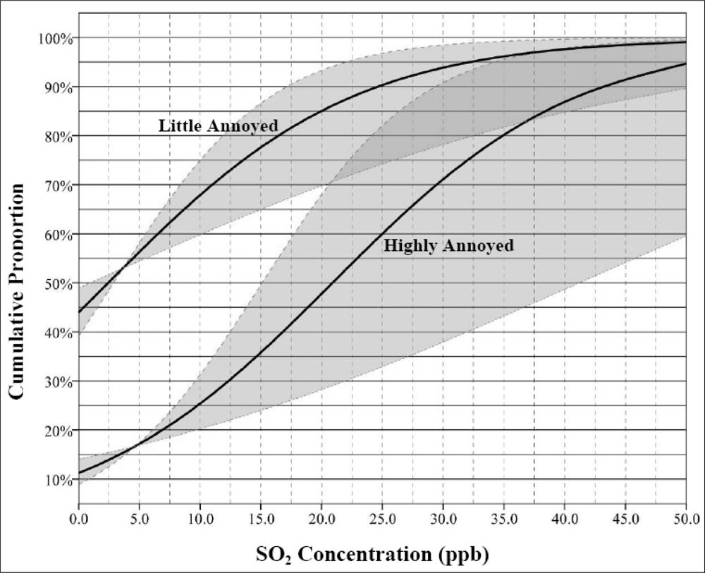
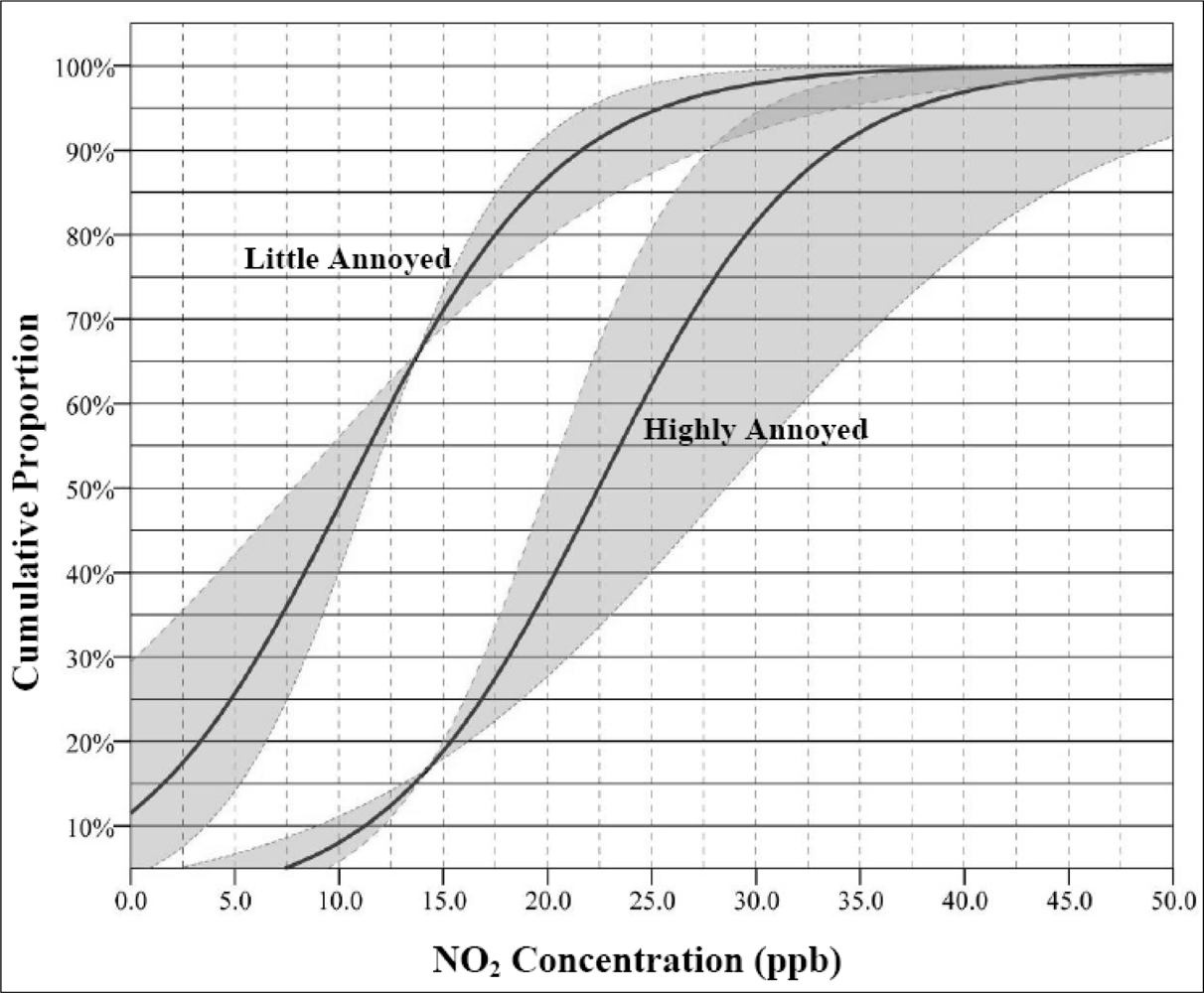
The result shows that about 8% of the respondents are highly annoyed at 10 ppb NO₂ exposure level. Figure 5 and 6 show the exposure – response relationship for NO₂ and SO₂ in the Sarnia respectively. The lower curve indicates the percentage of residents expected to be highly annoyed by given exposure levels from the industries. The upper curve is cumulative percentage of respondents who are at least a little annoyed. The gray bands indicate the 95% confidence intervals of the relationships between exposure and annoyance. These figures show quite large individual variation in reporting odour annoyance at given pollution levels (Figures 5 and 6). The figures indicate that, for example, at a 20 ppb NO₂ concentration levels, about 87% of respondents are at least a little annoyed while 37% of them are highly annoyed by industrial odour in their home addresses (Figure 5).

With the same concentration of SO₂ (20 ppb), at least 85% of respondents are a little annoyed and more than 47% are highly annoyed by odours in the region (Figure 6). The results show that many people are highly annoyed by SO₂ (47%) compared to NO₂ pollution (37%) at the same pollution concentration levels. At the same pollution levels, about 87 and 85% of Sarnia residents are at least a little annoyed to NO₂ and SO₂ pollution respectively. It should be noted that there are few or no concentrations for NO₂ above 17 ppb and above 12 ppb for SO₂ modelled concentrations. The range of 0–50 ppb was used to facilitate comparisons.

This study examines the relationship between odour annoyance and modelled pollution, exposure– response associations, and the determinants of annoyance scores in the highly exposed environment of Sarnia. Although modelled NO₂ and SO₂ concentrations are below Ontario’s AAQC, a considerable proportion of residents surveyed were annoyed by the odours. The study found a strong association between annoyance scores and the different LUR modelled ambient air pollutants including NO₂ and SO₂. Consistent with other studies [15,16], people who were exposed to high levels of modelled ambient air pollution reported high annoyance scores. Similarly, while Forsberg et al. reported high correlations between annoyance and NO₂, they found no significant relationship between annoyance scores and SO₂ concentrations in their study context [13]. When compared to our findings, the difference could be due to contextual factors. The Swedish study included several cities and towns across Sweden while this study is located in a relatively small and heavily industrial region with numerous petrochemical facilities.

We found significant correlation coefficients between odour annoyance and modelled pollutants (see Table 3). However, SO₂ concentration had higher coefficient (r = 0.67) compared to NO₂ (r = 0.56) at the census tract level. At the highly annoyed threshold (Figure 6), the results also showed that SO₂ cumulative exposure–response curve had wider variation compared to the NO₂ curve (Figure 5). These could likely be because individuals in the Sarnia area are more sensitive to SO₂ pollution which has a unique pungent odour compared to NO₂ which does not smell much. In this study, annoyance scores captured the within area variability of air pollution levels which suggests that odour annoyance is a function of real exposure and can be used as a proxy for air quality [13,15]. Consequently, where resources are limited, the establishment of expensive monitoring networks might not always be necessary because area variability of air pollution can be estimated in questionnaire surveys, where the marginal costs are low. The study showed that individual and mean census tract annoyance scores do reflect gradients of air pollution levels in Sarnia. However, the correlation coefficients between annoyance score and air pollution levels were improved when census tract level data were used. This finding suggests that exposure estimates based on census tract level would mitigate non-differential exposure misclassification [15,44]. We should however note that annoyance score can not replace personal exposure measurements, because of the high between-person variability of annoyance rating, which could partly be explained by the determinants of annoyance.

With the exception of gender, this study found no significant relationship between sociodemographic variables and odour annoyance scores (Tables 5 and 6). These findings are contrary to studies which reported, for example, that age, does significantly predict annoyance score reporting [10,45]. Luginaah et al. reported that young people were more likely to perceive odours and become annoyed than individuals who were older [26]. Furthermore, Steinheider [46] reported that age exerts an effect on olfactory sensitivity which results into the elderly having decreased sensitivity to odours. Although the descriptive statistics suggested a trend whereby older people were less likely to be annoyed by air pollution, the lack of significance in the multivariate analysis suggests the population in the Sarnia area which is constantly exposed to chronic odour and pollution may have been desensitized to exposure.

When examined in univariate analysis (not reported), health variables including self-assessed health status, chronic conditions, emotional distress, cardinal, and general health symptoms showed significant influence on the high annoyance reporting. However, when covariates were introduced, only cardinal symptoms reporting and their interaction with exposure to occupational dust showed significant influence on odour annoyance score reporting. These results signify the importance of covariates in modifying the influence of these health variables on odour annoyance reporting. Further, studies should explore how single health outcomes (e.g., asthma) rather than using composite health variables (e.g., chronic conditions) impact odour annoyance reporting. While examining the influence of individual health outcomes on self-reported air pollution problems, Piro et al. [9] found that people with chronic diseases (e.g., asthma, chronic heart disease) were more likely to report high odour annoyance.

Explaining the causal linkages between odour annoyance, odour perception, and health outcomes could be problematic. While examining the community reappraisal of perceived health effects of a petroleum refinery in Oakville, Ontario, Luginaah et al. [26] highlighted four possible causal mechanisms due to odour annoyance. First, there is a direct linkage between petrochemical facilities emissions and general health status. In fact, the industries were found to be significant contributors to the spatial variability of NO₂ and SO₂ pollution concentrations in Sarnia [33]. When compared, residents exposed to SO₂ were more likely to report higher annoyance scores than when they are exposed to NO₂ concentrations. This is partly because SO₂ and its reduced compounds (e.g., hydrogen sulphide) are known to produce pungent smells detectable at very low concentration levels and can directly result in ill-health such as nausea or headache [26]. In this study, we found significant relationships between modelled NO₂ and SO₂ pollution concentration, cardinal symptoms reporting, and odour annoyance scores suggesting that odour annoyance is influenced by pollution levels and other covariates. This finding is consistent with Luginaah et al.’s who found that strong odours may result in ill-health (e.g., nausea) reporting [26]. Second, the relationship between exposure and general health status may be mediated by odour perception. In such instances, respondents who negatively perceive odours are sensitized and are more likely to report ill-health and attribute them to the numerous industrial facilities in the region. Third, the direction of the relationship could be the reverse, such that respondents experiencing ill-health are sensitized to believe and be annoyed by odours from the industrial facilities. Finally, the relationship could be bidirectional, such that odour perception and self-assessed health reporting are mutually reinforcing each other.

Despite the fact that the models used in this study captured the significant proportion of the spatial variability of NO₂ and SO₂ in Sarnia [33], there are some limitations worth mentioning. First, there is the possibility that annoyance levels might be related to other pollutants that might be correlated to NO₂ and SO₂ concentrations but were not measured in this study. The use of a 6-digit postal code instead of personal monitoring to develop air pollution estimates might also be another limitation. Nevertheless, the findings make important contributions to the literature.

In general, this study provides strong support for the second mechanism, whereby the relationship between exposure to industrial pollutants including NO₂ and SO₂, and odour annoyance reporting is mediated by odour perception and health outcomes [26,30]. This mediating role is supported by the fact that when we controlled for perception of odours (including the belief that industrial odours impact health and odour have not improved in the last five years), for example, the odds of reporting high annoyance actually increased. This finding suggests that covariates (e.g., odour perception) are key modifiers of high annoyance reporting. Nevertheless, other odour annoyance mechanisms, outlined above, are also possible given that they are not necessarily mutually exclusive and that evidence from these results is not sufficient to reject them either. For example, we found that residents who reported two or more cardinal symptoms were more likely to report high odour annoyance. This finding is similar to Luginaah et al.’s [26] who report that adult cardinal symptoms are strong predictors of odour perception.

The exposure–response relationships indicate that residents of Sarnia are annoyed with pollution concentrations levels that are very low compared to the Ontario 24 hour allowable NO₂ and SO₂ concentration guidelines. Considering the relationship between odours mediated mechanisms and health effects, the results suggest the need to revisit the set guidelines for allowable exposure to pollution to better protect residents. This finding is consistent with Amundsen et al. [41] who found that people in Norway are annoyed to exposure levels that are commonly occurring in European cities even though they “satisfy” national and international guidelines for outdoor air pollution.

In conclusion, questionnaire-based odour annoyance score of ambient air pollution can be a useful proxy for assessing the within-area variability of air quality and measure of perceived ambient exposure and could be used for evaluating the implementation of environmental policies. In fact, as a subjective score of air quality, odour annoyance has been incorporated in the Swedish National Monitoring programs [10]. Odour annoyance can also be utilized as a complementary tool for determining exposure and concerns of residents in sentinel high exposure environments like Sarnia. There is need for policy makers to pay attention to residents’ complaints and concerns regarding pollution exposure for better policy implementation. Although subjective, annoyance scores from industrial odours do capture the intra-urban variability of ambient pollution. Since this study, to the best of our knowledge, is one of the first to validate the use of odour annoyance score in a Canadian industrial context, there is need to conduct longitudinal studies across different contexts and scales to further validate the use of annoyance scores as proxies for air pollution if there is the potential to adopt them at the national level.