1. Introduction
Hyperspectral data provide detailed spectral information about ground scenes based on a huge number of channels with narrow contiguous spectral bands. Hyperspectral data can therefore better discriminate the spectral signatures of land-cover classes that appear similar when viewed by traditional multispectral sensors [
1]. If successfully exploited, hyperspectral data can yield higher classification accuracy and more detailed class taxonomies.
However, this increase of data dimensionality has introduced challenging methodological problems because of the incapacity of common image processing algorithms to deal with such high-volume data sets [
2,
3]. In the context of supervised classification, the most common problem is the Hughes phenomenon [
4], implies that the required number of training samples for supervised classification increases as a function of dimensionality. One possible solution for mitigating the effects of the Hughes phenomenon is to reduce the dimensionality of the data but at the same time keep as much information as possible. For example, commonly used dimensionality reduction methods include feature selection and feature extraction methods [
5-
9], principal components analysis (PCA) with conventional classification methods [
10], Minimum Noise Fraction [
11], orthogonal subspace projection classification methods [
12], support vector machine (SVM) classifiers [
13-
18], and spectral angle mapper and spectral information divergence methods [
19,
20].
The subspace pattern recognition method is another dimensionality reduction method that can achieve dimension reduction and classification concurrently. The subspace method represents each class by a model of a linear subspace of a feature space. This method was originally proposed by Watanabe
et al. [
21]. In the subspace method, the original high-dimensional data are projected onto a low-dimensional space as done in PCA, but different classes are forced to follow different directions in this low-dimensional space. Subspace analysis has attracted much attention in the area of object recognition and character recognition during the last decade, and some examples are shown by Sakano
et al. [
22], and Omachi and Omachi [
23].
For character or face image recognition, the processing object is a binary image or a single-band gray-scale image, but for hyperspectral data, the object is a high-dimensional gray-scale image (dimensions equal to the number of bands). Thus, the subspace method must be extended accordingly to hyperspectral data classifications.
In the specific context of hyperspectral data classification, averaged learning subspace methods (ALSM) for hyperspectral data classification have been described by our previous work [
24]. The low-dimensional subspaces that can better characterize class information and can precisely distinguish it from other classes simultaneously. However, they provide results only by using a method of fixed subspace dimension and do not describe the behavior of the dimension selection or the parameter settings.
Moreover, several critical issues are still unclear, for example, (1) how the data normalization method affects the subspace method, (2) how various approaches for selecting subspace dimensions affect the classification accuracy, (3) how learning parameters influence the training speed and classification accuracy, (4) how the size of the training data set influences the classification accuracy, and (5) how to compute eigenvalues from the correlation matrices.
To avoid overflow problems, high-dimensional hyperspectral data need to be normalized to unit-length before one performs the subspace training and classification procedure. The primary objective of image normalization is to remove the effects of outliers by limiting the extent of scatterplot data [
25]. Some methods have been proposed for the normalization of satellite data for this purpose [
26]. We modified two commonly used normalization methods for hyperspectral data. A detailed description of the normalization methods will be addressed later.
Another major problem with subspace methods regards eigenvalue computation algorithms. The computational cost of subspace methods critically depends on the eigenvalue computation methods; thus, we adopted the QR method [
27] instead of the Jacobi method [
28].
In this paper, we present the dynamic subspace dimension method, which sets each subspace dimension independently in ALSMs (hereafter referred to as the dynamic subspace method), and the fixed subspace dimension method, which fixes subspace dimensions for each class as the same value as that used in ALSMs (hereafter referred to as the fixed subspace method) based on two normalization methods. We also carried out experimental studies on 16 land-cover classes using the “Indian Pines” 92AV3C9 data set collected from the Airborne Visible/Infrared Imaging Spectrometer (AVIRIS) hyperspectral sensor of June 1992 for the Indian Pines area, Indiana, USA (
http://dynamo.ecn.purdue.edu/~biehl/MultiSpec) [
29]. Different performance indicators are used to support our experimental analysis, namely, the classification accuracy, computational cost, stability of dimensions selection, and learning parameter settings. Experimental results confirm the considerable advantage of the subspace method in the context of hyperspectral data classification. Since many previously published classification methods used the Indian Pines data sets for experiments, e.g., SVM methods [
5,
13,
14] and feature selection and feature extraction methods [
6,
8,
17]. Therefore it is convenient for the reader to compare the proposed subspace methods described herein with those approaches
The rest of this paper is organized as follows. First, we describe the main idea of subspace methods. Next, we present the data sets and associated processing steps, i.e., normalization methods and eigenvalue computation algorithms. Then, we show comparison results and analyses for AVIRIS hyperspectral data experiments between different normalization methods and our subspace methods. Finally, we present concluding remarks.
2. Subspace Methods
2.1. CLAFIC and ALSM Subspace Methods
Subspace methods have been extended in many ways. The most basic is called class-featuring information compression (CLAFIC) [
30], the procedure of which is as follows.
Assume that available hyperspectral data from a given site contain n bands, the implicit pixels are of an n-dimension column vector, and user-defined classes of ω(1), ω(2), …, ω(K) appear. A set of labeled pixels for all such classes should also be available, divided into training and test data sets.
Given a set of training samples sk,i∈Rn (1 ≤ i ≤ p) that belong to class ω(k) (1 ≤ k ≤ K), where n same as the number of bands in a hyperspectral data set, p represents the total number of training samples in class ω(k), and K denotes the number of classes, let rk denote the number of dimension of the subspace Dk(⊂ Rn) of class ω(k) for which rk < min(n, p) is satisfied. Let Tk=(tk,1, …, tk,k) denote the base vectors matrix of subspace, where tk,i is the i-th normal orthogonal base.
Dk is included in the subspace spanned by the training sample
sk,i (1 ≤
i ≤
p), thus the bases can be represented by
Where:
in which
uk,i,j are coefficient parameters and
Uk,i=(
uk,i,1, …,
uk,i,p)
T are coefficient vectors.
For the recognition (classification) task, one needs to compute the distance between the pattern vector (pixel)
v and each subspace, and label
v into the classes that have the shortest distances. It is formulated by:
which becomes:
Hence, finding the shortest distance is equivalent to finding the largest squared length of the orthogonal projection between pattern vector v and each subspace.
Combining
equations (2) and
(7), we get:
where
SkTv is a dot product matrix between the pattern vector
v and the training sample matrix.
Equation 8 is equivalent to finding
Uk that maximizes:
subject to:
where
I is an n×n unit matrix. The optimal solution to this problem is given by the following theorem.
Theorem
Let
Pk =
SkTSk and let the first
rk largest corresponding eigenvalues be arranged in descending order:
λk, 1≥
λk, 2≥, …, ≥
λk, rk (>0). Let the corresponding eigenvectors be denoted by
αk,1,
αk,2,
αk, rk. The optimum solution of
equation (9) is:
The proof is shown by Tsuda [
31].
In summary, determining the subspace of class ω(k) is to solve the eigenvalue problem of matrix SkTSk. Here SkTSk is the sample correlation matrix from those whose eigenvalues and eigenvectors can be computed by some existing method such as the Jacobi or QR method. The eigenvectors αk,1, αk,2, αk, rk of SkTSk are computed corresponding to the first rk largest eigenvalues. Then these eigenvectors comprise the subspace Dk of k-th class ω(k).
CLAFIC has the drawback that subspaces obtained for one class are not dependent on subspaces of other classes. To avoid this problem, an iteration-learning algorithm, called the ALSM has been proposed [
30,
32]. In this method, the subspaces are suitably rotated in each iteration training step. When an error occurs in the ALSM, the correct subspace is rotated toward the misclassified vector and the wrong subspace is rotated away from it. This is achieved by modifying the class conditional correlation matrices and then updating the basis vectors of subspaces.
At each step
k, one divides the misclassified training samples into two types: either a sample vector of class
ω(i) is misclassified into another class, say
ω(j), or a sample vector of another class, say
ω(k), is misclassified into class
ω(i). We denote the conditional correlation matrix by:
where the symbol ↦ denotes the sample that has been misclassified into class
ω(j). Based on current existing subspaces, all training samples are classified according to
equation (7), and all matrices
Pk(i,j),
i, j = 1, 2, …,
K are computed. Then, the correlation matrices for each class are computed as:
where
α and
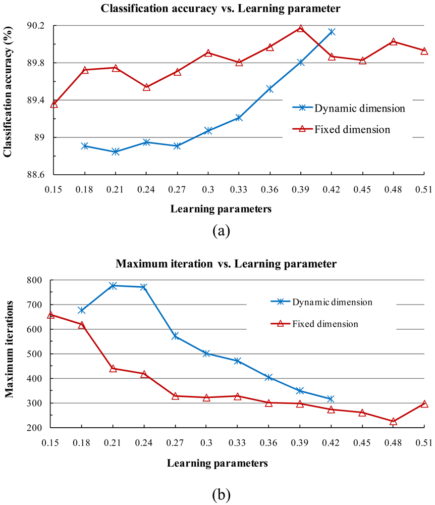
β are the learning parameters, which are usually set to two constant values and do not vary in the iteration process. Then a new subspace of class
ω(i) can be computed from
Pk(i).
2.2. Subspace Dimension
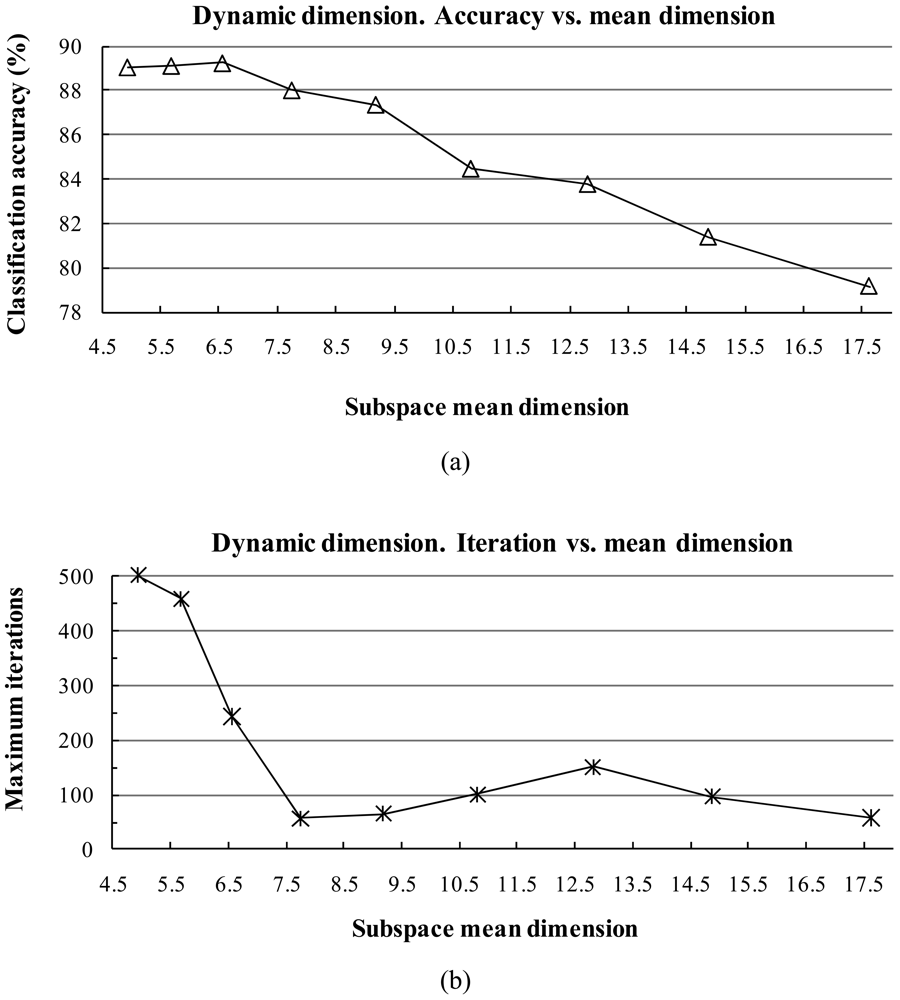
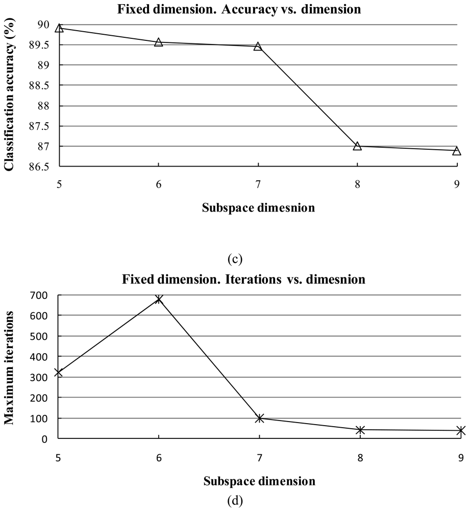
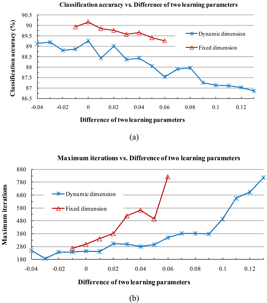
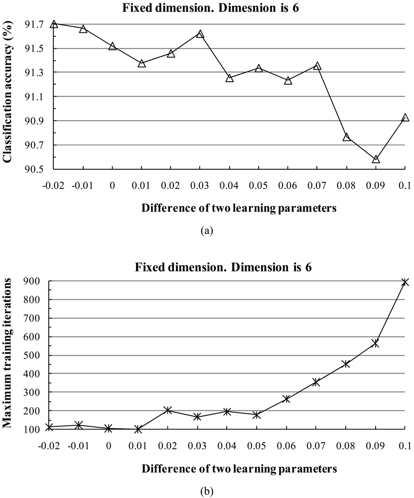
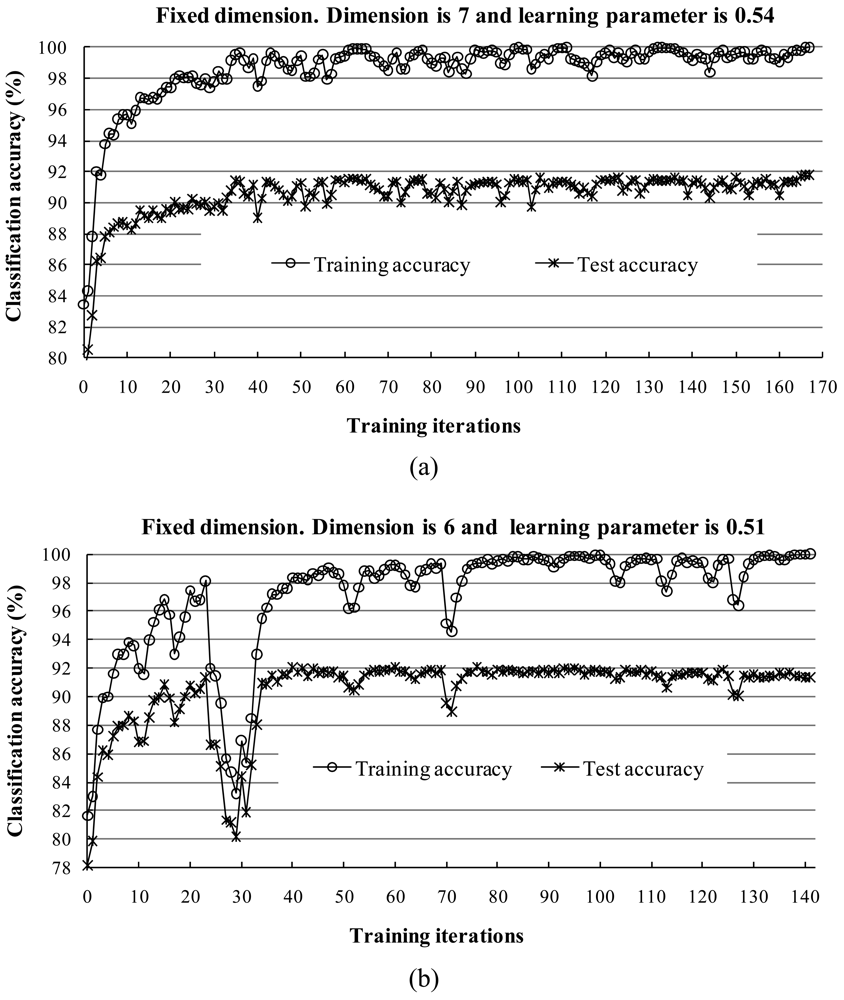
The subspace dimension markedly affects the pattern recognition rate. The dimensionalities of class subspaces are decided in the CLAFIC stage and then are kept constant during the learning process. Methods for selecting the dimension can be divided into two types: (1) fixed subspace methods, which set a uniform dimension for all classes, and (2) dynamic subspace methods, which set subspace dimensions differently for each class.
For dynamic subspace methods, the selection of the dimension
ri (1 ≤
I ≤
c) of each subspace
ω(i) can be chosen based on a fidelity value (i.e., threshold)
η (0 <
η ≤ 1) as follows:
where eigenvalues are sorted in descending order. The fidelity value decides the degree of overlap between the subspaces. The classification accuracy is sensitive against the fidelity value.
3. Preprocessing Methods and Data Sets
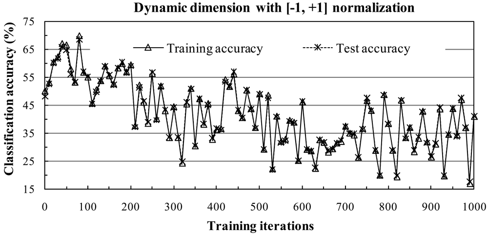
In this section, we compare the proposed ALSM classification systems with two different normalization methods developed for ALSM. In the two normalization methods, we use them to normalize each pixel to a unit-length vector by dividing each element according to the vector length. This method can avoid the influence of noise pixels, since it does not use the values of neighboring pixels. Detailed descriptions of the two normalization methods are as follows.
3.1. Normalization Methods
Since high-dimensional hyperspectral data are usually at least 10 bits in size, the cumulative values of original high-dimensional hyperspectral data may cause overflow problems when we compute eigenvalues and eigenvectors from the correlation matrix in the ALSM training process without normalization. Hence, normalization is an important step of the algorithm.
There are many normalization methods. In this section, we only consider the [-1, +1] and [0, 1] normalization methods. The choice of scaling each attribute to the range [-1, +1] or [0, 1] is motivated by the successful application of the method to SVM classifiers [
33].
In the [0, 1] normalization method, data are normalized to the range [0, 1] as follows: Given a pixel
s = (
s1,
s2, …,
sn)
T, a normalized pixel is computed as:
where d = sqrt(
s12+
s22+…+
sn2) denotes the pixel length. Obviously, each element value of the normalized pixel is located within the range [0, 1] and the length of the pixel is 1.
In the [-1, +1] normalization method, data are normalized to the range [-1, +1] and the scale can be adjusted such that the mean of the data is equal to zero. The [-1, +1] normalization procedure is given as follows: Given a pixel
s = (
s1,
s2, …,
sn)
T, we compute:
where
s′ = (
s′
1,
s′
2, …,
s′
n)
T denotes the normalized pixel. Note that
s′
1+
s′
2+…+
s′
n = 0 if (
s′
1-
m)
2+(
s′
2-
m)
2+ …+(
s′
n-m)
2 = 0.
3.2. Eigenvalue Computation Methods
Computing the eigenvalues and eigenvectors of the correlation matrix of the input data vector (training samples) is a time-consuming process since the correlation matrix can be as large as bands × bands of elements in hyperspectral data. The time can be noticeably shortened by choosing an appropriate eigenvalue computation algorithm.
Let A be an
n×
n real or complex matrix whose eigenvalues we seek. The eigenvalue
λ of
A satisfies
Ax =
λx, and can be computed from the characteristic equation det(
A −
λI) = 0. Notice that the correlation matrices in
equations (14) and
(15) are real symmetric matrices. For a real symmetric matrix, there exists an orthogonal matrix
Q, such that
QTAQ =
D, where
D is a diagonal matrix. The diagonal elements of
D are the eigenvalues of
A, and the columns of
Q are the corresponding eigenvectors of
A. The Jacobi and QR methods are two of the most useful algorithms for solving eigenvalue problems. In the Jacobi method, which was originally proposed in 1846, a real symmetric matrix is reduced to a diagonal form by a sequence of plane rotations by orthogonal similarity transformations. The QR method works much faster on a dense symmetric matrix for computing eigenvalues and associated eigenvectors. The basis of the QR method for calculating the eigenvalues of
A is that an
n ×
n real symmetric matrix can be written as
A =
QR where
Q is an orthogonal and
R is an upper triangular matrix. The diagonal elements of
R are the eigenvalues, and the columns of
Q are the corresponding eigenvectors. Here, we adopt the
QR algorithm instead of the Jacobi algorithm for eigenvalue computations. The
QR algorithm dramatically reduced, by approximately 75%, the time cost of computing eigenvalues in our study. According to recent research, other faster eigenvalue computation algorithms could be adopted [
34].
3.3. Data Sets and Experimental Settings
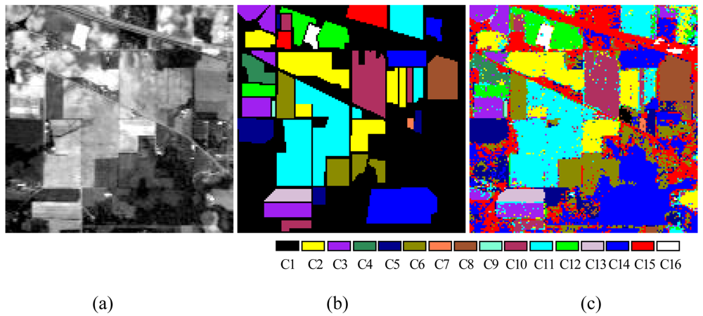
To verify the performance of the proposed ALSM algorithm, simulations were carried out on the “Indian Pine” AVIRIS 92AV3C data set, which consists of a 145 × 145 pixel portion [see
Figure 7(a)]. The data set was collected over a test site called Indian Pine in northwestern Indiana, USA, by AVIRIS sensors in June 1992. From the 220 original spectral bands, 29 atmospheric water absorption bands (1–3, 103–109, 149–164, and 218–220) were removed, leaving 191 bands. These data values in the scene are proportional to radiance values. Labeled ground truth samples were obtained based on the previous information collected at the Laboratory of Remote Sensing at Purdue University (
http://dynamo.ecn.purdue.edu/~biehl/MultiSpec) [see
Figure 7(b)] [
29]. All 16 land-cover classes available in the accompanying original ground truth were used in our experiments to generate a set of 9,782 pixels for training and testing sets. A simple random sampling method in which each sample had an equal chance of being selected was used for generating training and testing sample sets. Half of the pixels from each class were randomly chosen for training, while the remaining 50% formed the test sets (
Table 1).
To avoid the possibility of overflow problems when computing eigenvalues and eigenvectors, all images, training data, and test data were normalized by the [-1,+1] and [0,1] normalization methods. Experiments with various parameter values were necessary to develop a reasonable subspace classifier. The following section describes the design and results these experiments.


