1. Introduction
HF radar systems are widely used internationally to provide continuous monitoring of ocean waves and currents for a large range of environmental conditions.
Within the US, coastal ocean current mapping with HF radar has matured to the point where it is now considered an important component of regional ocean observing systems. A mid-Atlantic HF radar network now provides high resolution coverage within five localized networks, which are linked together to cover the full range of the mid-Atlantic coastal ecosystem. Similar regional networks around the US coastline are being formed into a national HF radar network.
While much of the focus of these networks until now has been on offshore current mapping observations, a longer-term objective is to develop and evaluate near-shore measures of waves and currents. These investigations aim to understand the interaction of waves in the shallow coastal waters and how energy is transformed into the creation of dangerous rip currents along the New-Jersey/Long-Island shorelines. Rutgers University radars cover these coastal regions at multiple frequencies from 4.5 to 25 MHz. Their echoes contain information on both currents and waves from deep water up into the shallow coastal zone, providing an excellent archive for such studies. This paper describes the analysis of both simulated and measured radar echo to demonstrate the effect of shallow water on radar observations and their interpretation.
Radar sea-echo spectra consist of dominant first-order peaks surrounded with lower-energy second-order structure. Analysis methods presently in use assume that the waves do not interact with the ocean floor, see [
1,
2,
3] for phased-array-antenna beam-forming systems; and [
4] for systems with compact crossed-loop direction-finding antennas, such as the SeaSonde.
The assumption of deep water is often invalid close to the coast and for broad continental shelves, and is particularly inadequate to describe the second-order sea-echo used to give information on ocean waves., as second-order echo is often visible above the noise only for close ranges. To interpret this echo correctly, we show that the effects of shallow water must be taken into consideration.
In Section 2, we give the basic equations describing radar echo from shallow water, expanding on the previous description given in [
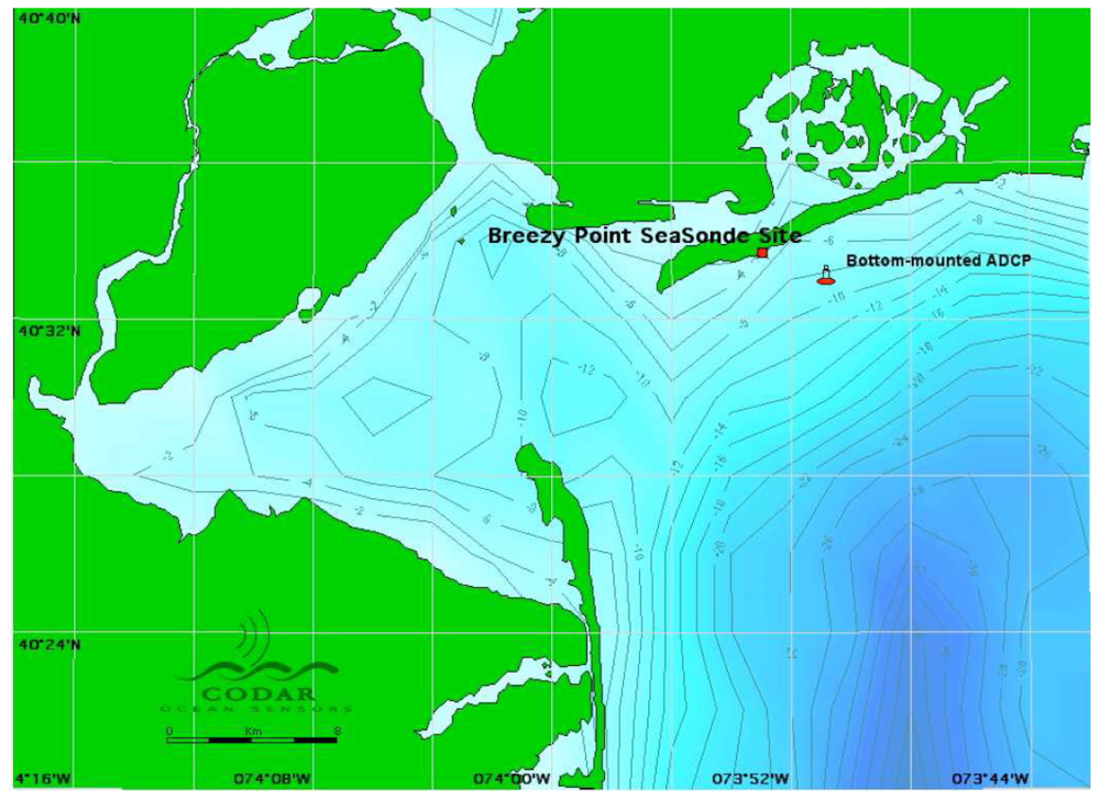
5]. In Section 3, simulations are used to illustrate the effects of shallow water on waveheight, Doppler shifts and spectral amplitudes in radar sea-echo spectra, to investigate limits on the existing theory and to define depth limits at which shallow-water effects must be included in the analysis. The effects of shallow water on the radar spectrum are illustrated using measured spectra. In Section 4, methods are applied to the interpretation of measured radar echo from a Rutgers University radar to produce wave directional spectral estimates, which are compared with wave observations from a bottom-mounted Acoustic Doppler Current Profiler (ADCP) moored in the second radar range cell.
2. Radar spectral theory
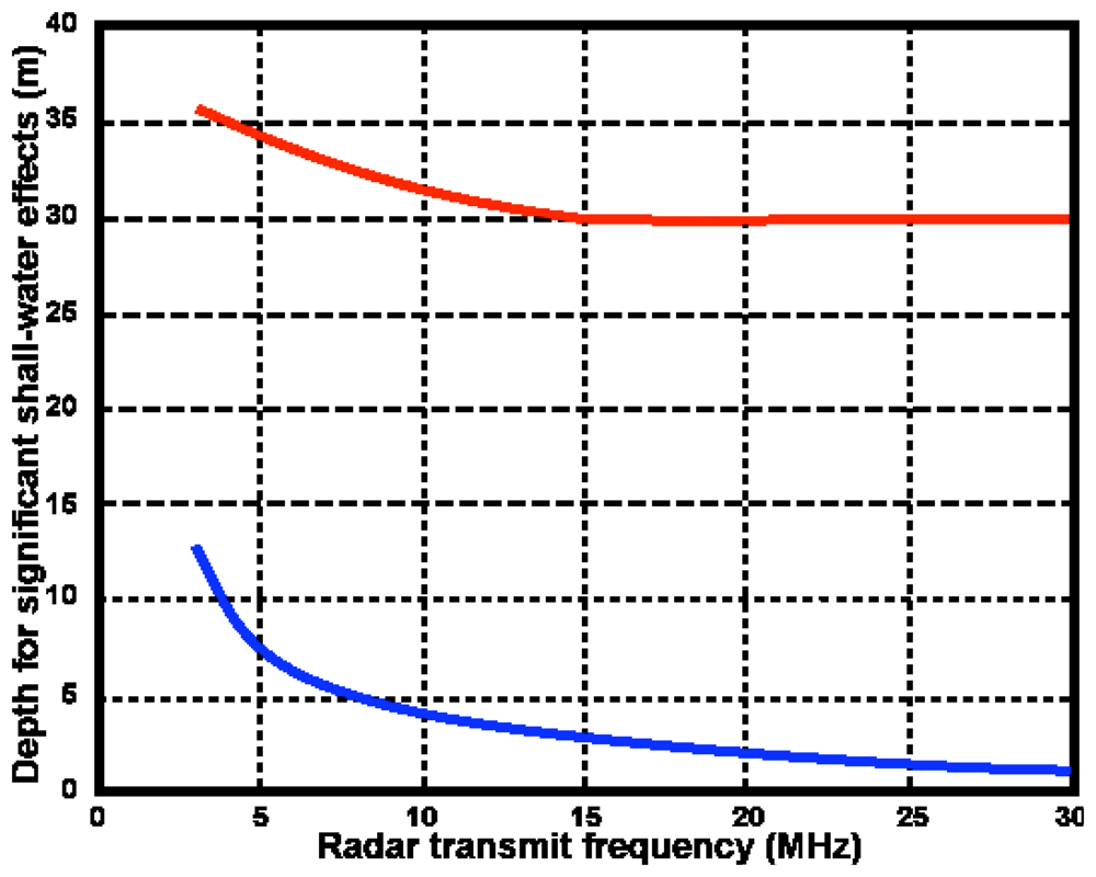
It follows from the solution of the equations of motion and continuity that long ocean waves are more affected by shallow water. We define the depth at which waves interact with the ocean floor by the approximate relation:
where
d is the water depth and
L is the dominant ocean wavelength. The deep-water analysis must be modified to allow for shallow-water effects in the coupling coefficients, the dispersion equation refractive effects on wave direction, and the directional ocean wave spectrum itself. We only consider water of sufficient depth that effects of wave energy dissipation such as breaking and bottom friction may be ignored; thus we operate in the linear wave transformation regime. As a general rule, this assumption is valid when the water depth is greater than 5% of the deep-water wavelength.
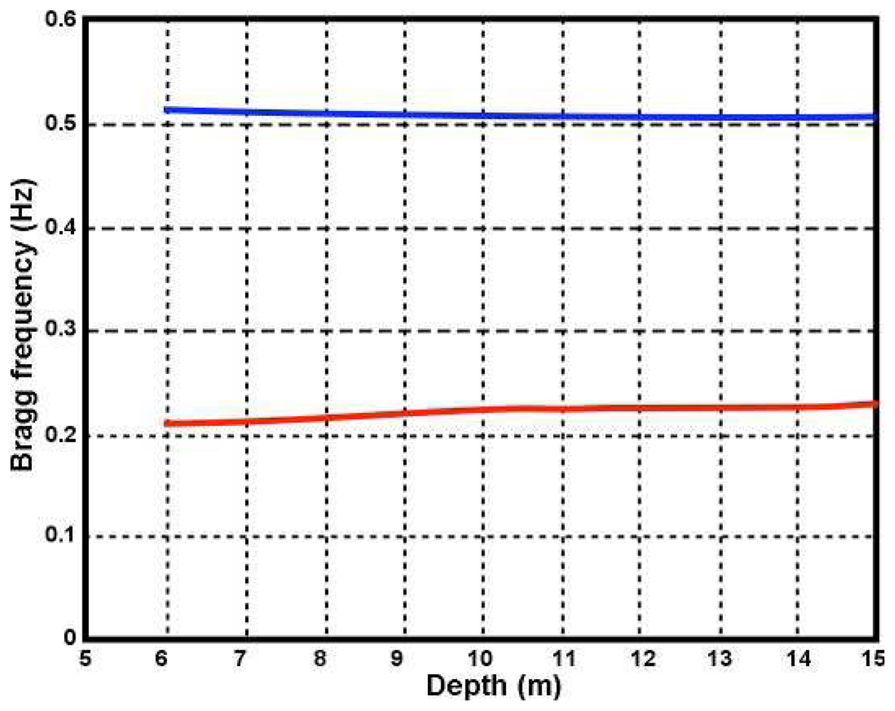
Applying the lowest-order shallow-water dispersion equation to first-order backscatter from the sea gives the following equations for
, the first-order spatial wave vector and
, the temporal wavenumber of the ocean waves in shallow water producing the backscatter. In this document, a subscript or superscript s indicates a shallow-water variable; its absence indicates a deep-water variable.
where
k̃0 is the radar wave vector, of magnitude
k0 ,
ωB and is the Bragg resonant frequency in shallow water which is given by:
with
g the gravitational constant. The analogous relations for second-order backscatter are:
Where
k̃s,
k̃s are the spatial wavevectors (with magnitudes
ks,
) of the two shallow-water, first-order ocean waves interacting to produce the second-order backscatter.
m,
m′ are equal to +1, -1 for waves moving toward, away from the radar respectively.
The electromagnetic coupling coefficient has the same form as for deep water [
5] but with shallow-water wavevectors:
where Δ is the normalized surface impedance. The hydrodynamic coupling coefficient, derived by Barrick and Lipa [
6] through solution of the equations of motion and continuity, is a function of water depth:
where k and k′ are the spatial wavenumbers of the scattering waves in deep water. The deep- and shallow-water spatial wavenumbers are related as follows:
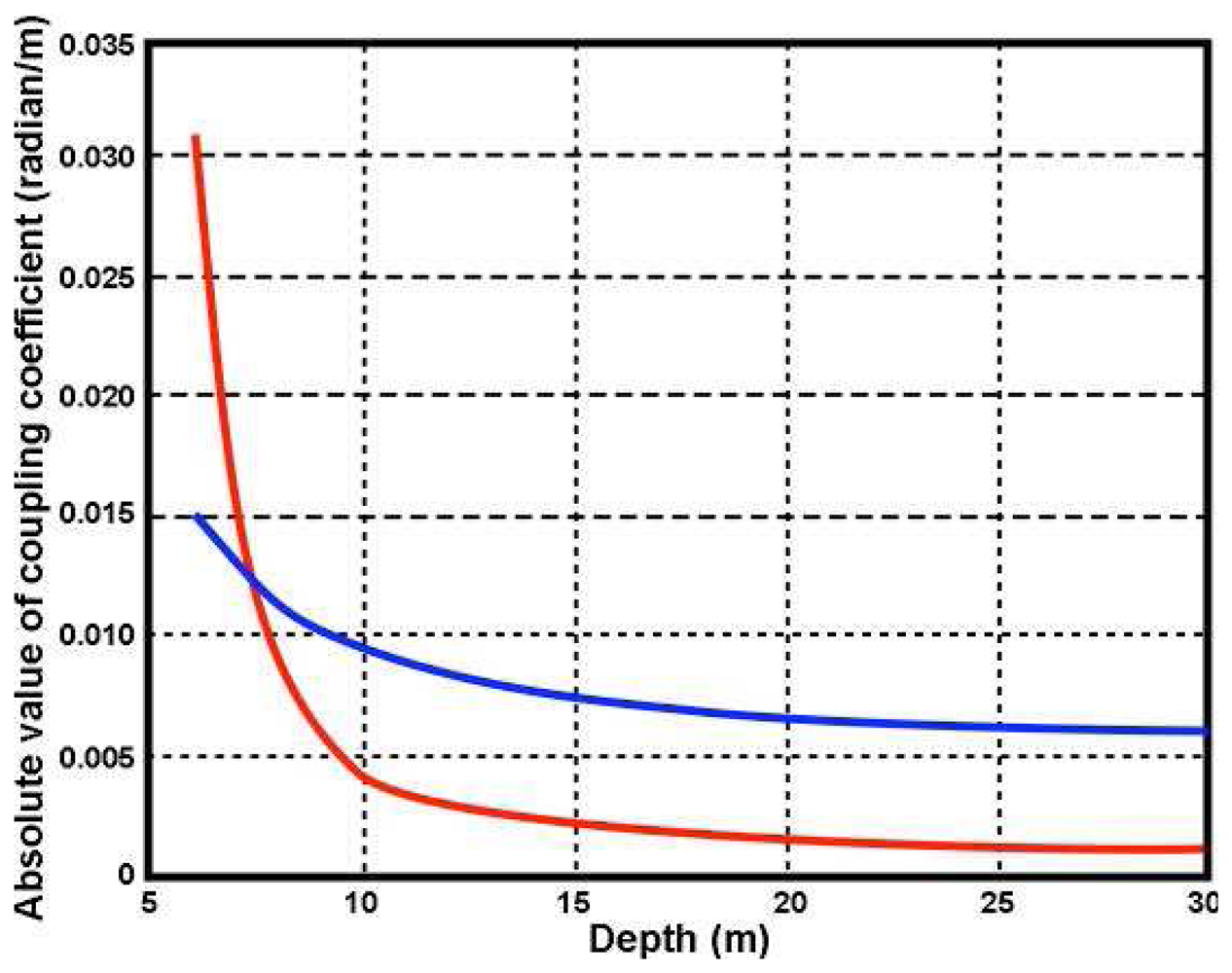
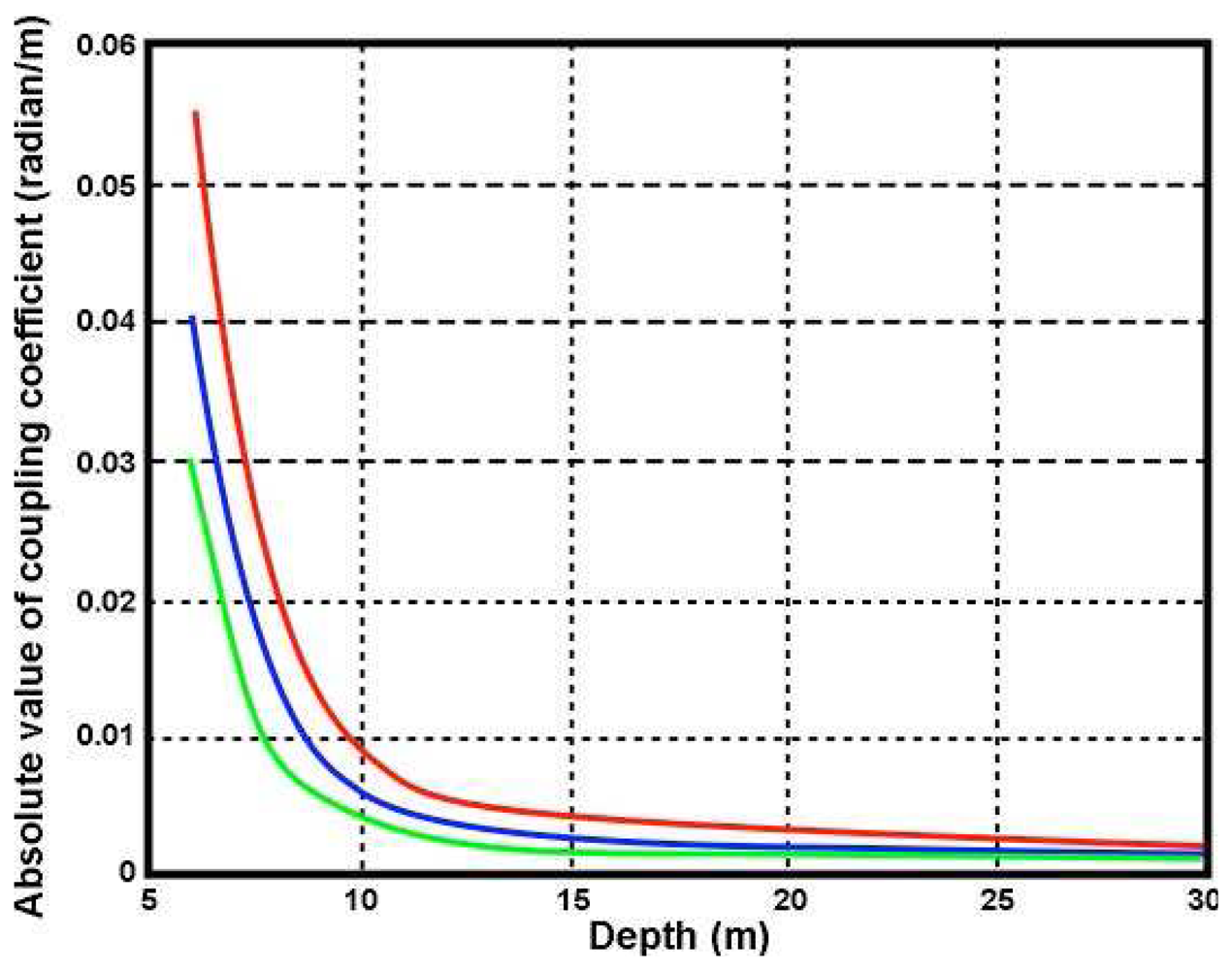
The total radar coupling coefficient Γ
s is the coherent sum of the hydrodynamic and electromagnetic terms
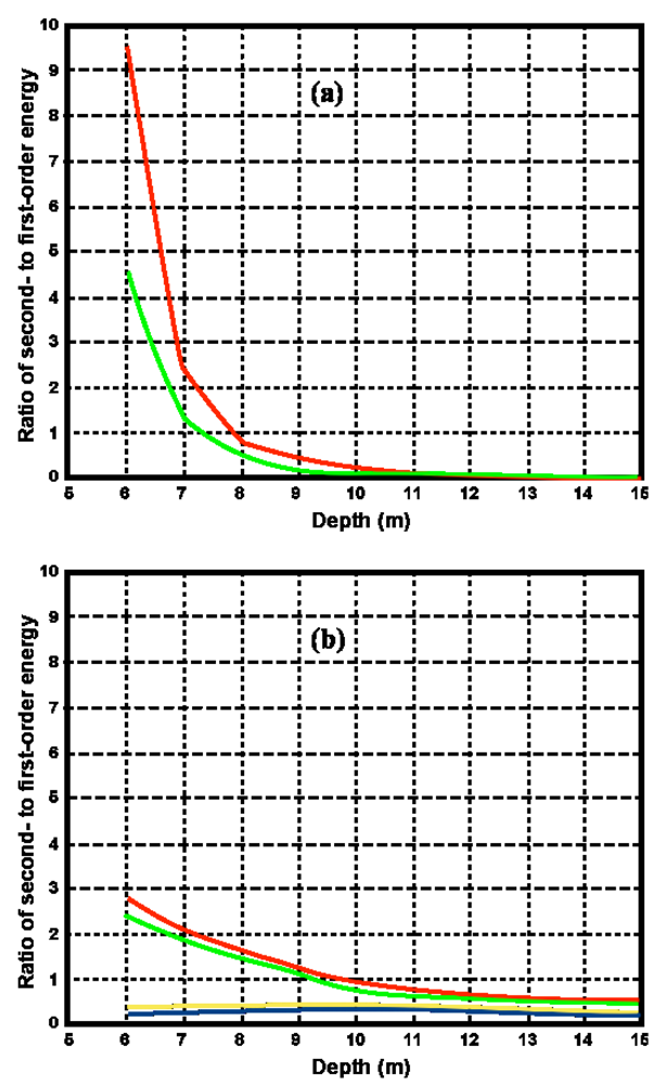
It can be shown from these equations that at constant wavenumber, the coupling coefficient increases as the water depth decreases, resulting in an increasing ratio of second- to first-order energy as the depth decreases.
In the following analysis, we assume that the deep-water directional wave spectrum is spatially homogeneous and that any inhomogeneity in shallow water arises from wave refraction. When energy dissipation can be neglected, it follows from linear wave theory that since the total energy of the wavefield, is conserved, the shallow-water wave spectrum expressed in the appropriate variables is equal to the deep-water spectrum [
7]:
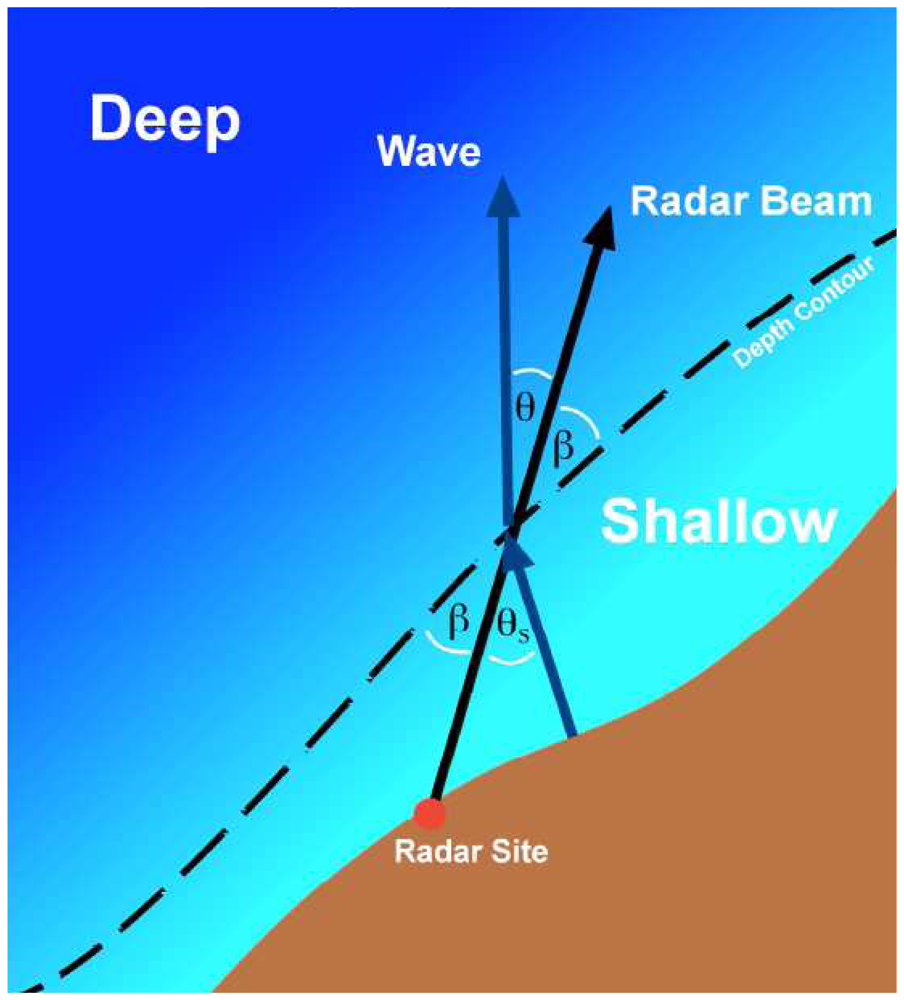
where the deep- and shallow-water wave vectors are related by Snell's law and the dispersion equation:
Here
β is the angle between the radar beam and the depth contour and
θs ,
θ are the angles between the radar beam and the shallow-, deep-water ocean waves respectively.
Figure 1 illustrates refraction at a contour between regions of differing depth.
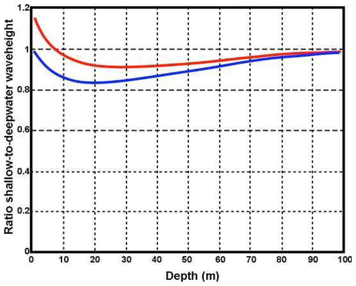
The shallow- and deep-water rms waveheights are given by:
Substituting
(10) and
(11) into
(12) gives the following relations which are useful for deriving the shallow- from the deep-water wave spectrum and vice versa:
where the Jacobian
J(
ks,
θs) is given by:
The first- and second-order radar cross sections in shallow water at frequency
ω and azimuth angle
φ are given by:
where
Ss(
k, α)) is the directional ocean wave spectrum for wavenumber k and direction
α□.
where the coupling coefficient Γ
s is given by
(8). The values of m and m′ in
(16) define the four possible combinations of direction of the two scattering waves. Common numerical multiplicative constants in
(15) and
(16) have been omitted. It can be shown from
(4) that the wavenumbers of the scattering waves are related as follows:
To compute the second-order integral in
(16), we choose as integration variables
ks and the deep-water angle
θ. In terms of these variables
(16) becomes
where
and
and where we have substituted
(9) for the shallow water directional spectra. The factors
and
are obtained by differentiation using
(10),
(11) and
(19).
To calculate the integral in
(18), it is first reduced to a single-dimensioned integral using the delta function constraint. The remaining integral is computed numerically.
Frequency contours are defined by:
which is solved for
k as a function of
θ for a given value of
ω. Due to wave refraction, the shallow water angle and wavenumber have discontinuities when the deep-water wave moves parallel to the depth contour, i.e. when
where
β is the angle between the radar beam and the depth contour.
Frequency contours are hence also discontinuous due to this effect at deep-water wave angles defined by
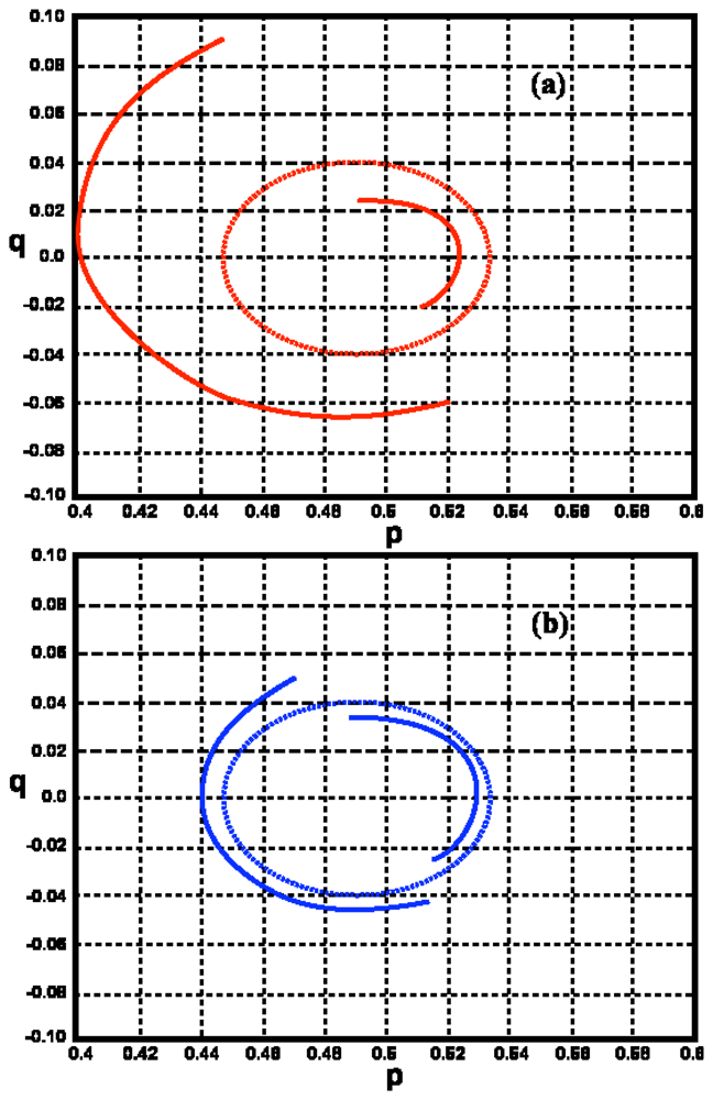
(22). Examples of frequency contours for deep- and shallow-water are shown in
Figure 2, plotted in normalized deep-water spatial wavevector space
k̃ / (2
k0). Normalized components
p,
q are defined so that
p is along the radar beam and
q perpendicular:
The discontinuities in the frequency contours are more pronounced when the contour is drawn in shallow-water wavenumber space, as it follows from
(10),
(11) that there are discontinuities in the shallow-water wave angle due to wave refraction.
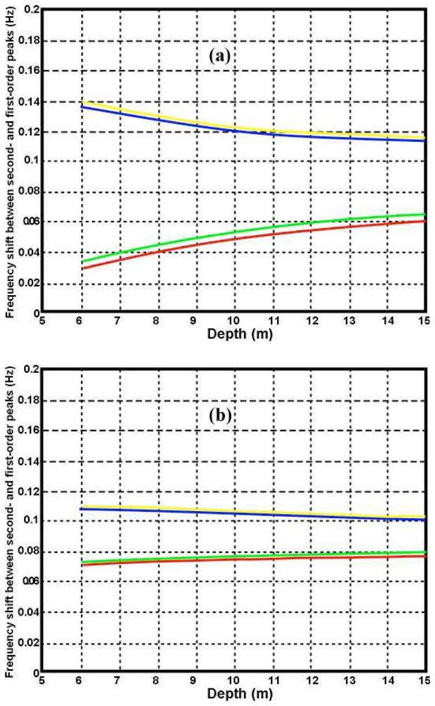
It can be seen from
Figure 2 that the deep-water ocean wave numbers corresponding to a given radar spectral frequency change with depth: they become either greater or smaller than the deep-water values, depending on the wave direction. This results in the frequency of second-order peaks in the radar spectrum changing with water depth.
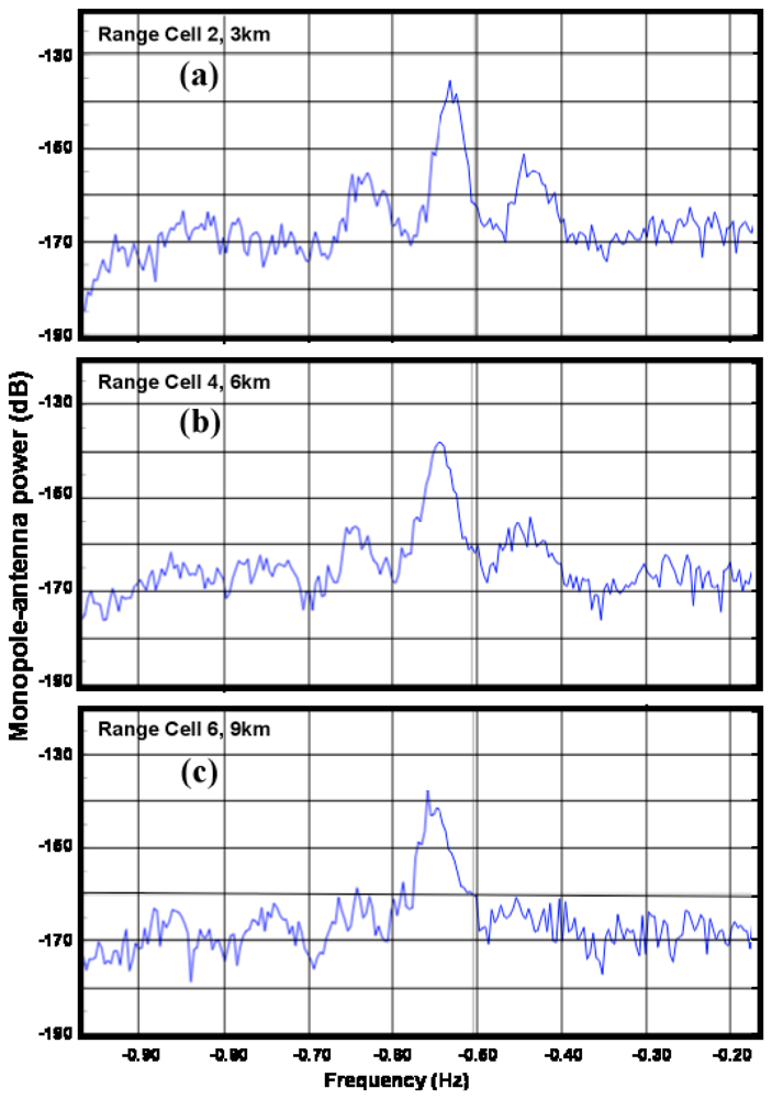
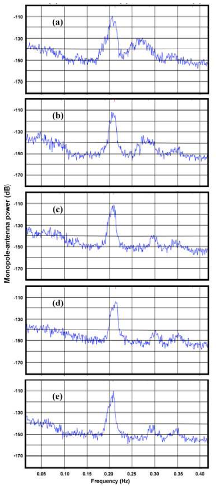
The effects of shallow-water on measured radar spectra are illustrated in
Figure 3, which shows measured spectra from a 5 MHz radar in five radar range cells, with distances ranging from 18km to 60km. As the water depth decreases, the second-order energy increases relative to the first-order and the frequency displacement between the first- and second-order peaks decreases. In the outer ranges, the second-order structure is almost the same from range cell to range cell, as the water is effectively infinitely deep.


