Here we present a few of our latest results by using our VLF/LF radio sounding. First, we present a result on the statistical correlation of ionospheric perturbations as detected by subionospheric VLF/LF radio sounding with the earthquakes. Then, we present a case study as detected in Japan for the huge Indonesia Sumatra earthquake.
3.1. Statistical study on the correlation between ionospheric perturbations and earthquakes
In addition to the event studies it is highly required to undertake any statistical study on the correlation between ionospheric disturbances and earthquakes based on abundant data source. There have been very few reports on the statistical correlation between the ionospherc perturbations and earthquakes (
Shvets et al., 2002,
2004b;
Rozhnoi et al., 2004).
Shvets et al. (2004b) have examined a very short-period (March-August, 1997) data for two paths (one is the Tsushima-Chofu and another, NWC (Australia)-Chofu) and found that wave-like anomalies in VLF Omega signal with periods of a few hours (as indicative of the importance of atmospheric gravity wave as suggested by
Molchanov et al., 2001;
Miyaki et al., 2002) were observed 1-3 days before or on the day of moderately strong earthquakes with magnitudes 5-6.1. Then,
Rozhnoi et al. (2004) have extensively studied 2 years data of the subionospheric LF signal along the path Japan (call sign, JJY)-Kamchatka (distance = 2,300 km), and have found from the statistical study that the LF signal effect is observed only for earthquakes with magnitude, at least, greater than 5.5.
The following is a summary of our latest paper (
Maekawa et al., 2006) devoted to such a statistical study on the correlation between ionospheric disturbances and seismic activity. A few important distinction from the previous works by
Shvets et al. (2002,
2004b) and
Rozhnoi et al. (2004) are described. The first point is the use of much longer period of VLF/LF data (five years long). The second point is that we pay attention to physical parameters of VLF/LF propagation data; (1) amplitude (or trend) and (2) dispersion (in amplitude) (or fluctuation). In the previous work by
Rozhnoi et al. (2004) they have studied the percentage occurrence of anomalous days, in which an anomalous day is defined as one day during which the difference of amplitude (and/or phase) from the monthly average exceeds one standard deviation (σ).
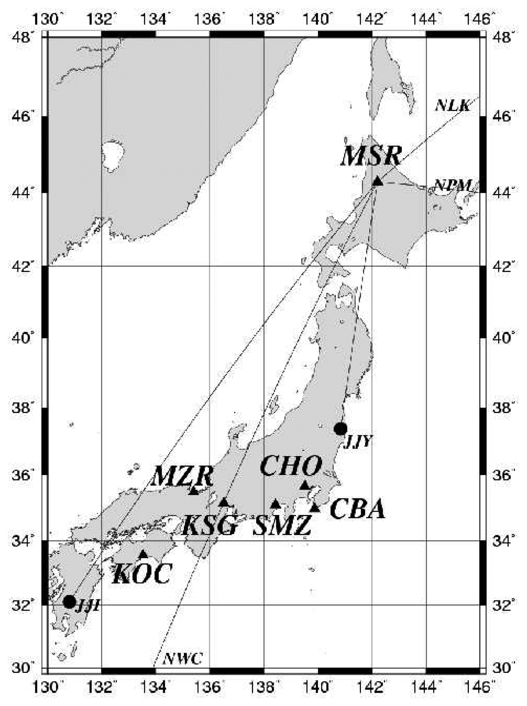
Here we pay particular attention to the earthquakes occurring in and around Japan, so that we take a wave path from the Japanese LF transmitter, JJY (40 kHz) (geographic coordinates; 36°18′ N, 139°85′ E) and a receiving station of Kochi (33°33′ N, 133°32′ E).
Fig. 3 illustrates the relative location of the LF transmitter, JJY and our receiving station, Kochi, and the distance between the transmitter and receiver is 770 km.
The subionospheric LF data for this propagation path is taken over 6 years from June 1999 to June 2005, but we excluded one year of 2004 (January to December, 2004) because of the following reason. As you may know, there was an extremely large earthquake named 2004 Mid Niigata prefecture earthquake happened on October 23, with magnitude = 6.8 and depth = 10 km (
Hayakawa et al., 2006), and the effect of the main shock and also large aftershocks was so large and so frequent that it may disturb our following statistical result so much. Then we have excluded this year of 2004 from our analysis. We have to define the criterion of choosing the earthquakes. The sensitive area for the wave path, JJY transmitter to the Kochi receiving station is defined as follows. As shown in
Fig. 3, first we adopt the circles with radius of 200 km just around the transmitter and receiver, and then the sensitive area is defined by connecting the outer edges of these two circles. All of the 92 earthquakes with magnitude (conventional magnitude (M) by Japan Meteorological Agency) greater than 5.0 are plotted in
Fig. 3, but the earthquake depth is chosen to be smaller than 100 km (with taking into account our previous result that shallow earthquakes can have an effect onto the ionosphere by
Molchanov and Hayakawa (1998)). We have normally been using the fifth Fresnel zone as the VLF/LF sensitive area (
Molchanov and Hayakawa, 1998;
Rozhnoi et al., 2004), but we have found that the area just around the transmitter and receiver is also sensitive to VLF perturbation (e.g.
Ohta et al., 2000) with taking into account the possible size of the seismo-ionospheric perturbation. In this sense the sensitive area we choose here seems to be very reasonable because the width of the sensitive area is very close to the 10th Fresnel zone.
In the following statistical analysis, we undertake the so-called superimposed epoch analysis in order to increase the S/N ratio. Here we define the earthquake magnitude in the following different way. Because we treat the data in the unit of one (a) day (we use U. T. (rather than L. T.) to count a day because we stay on the same day even when we pass the midnight when we use U.T.), we first estimate the total energy released from several earthquakes with different magnitudes in one day within the sensitive area for the LF wave path as shown in
Fig. 3 by integrating the energy released by a few earthquakes (down to the conventional magnitude M = 2.0) and by converting this into an effective magnitude (Meff) for this particular day. This Meff is much more important than the conventional magnitude for each earthquake, because the LF propagation anomaly on one day is the effect integrated over several earthquakes taking place within the sensitive area on that day. Though not shown as a graph, we find that there are 19 days with Meff greater than 5.5.
Diurnal variations of the amplitude and phase of subionospheric VLF/LF signal are known to change significantly from month to month and from day to day. Therefore, following our previous works (
Shvets et al., 2002,
2004a,
b;
Rozhnoi et al., 2004;
Hayakawa et al., 2006;
Horie et al., 2007a), we use, for our analysis, a residual signal of amplitude dA as the difference between the observed signal intensity (amplitude) and the average of several days preceding or following the current day:
where A(t) is the amplitude at a time t for a current day and <A(t) > is the corresponding average at the same time t for ±15 days (15 days before, 15 days after the earthquake and earthquake day). In the paper by
Rozhnoi et al. (2004), they have defined an anomalous day when dA(t) exceeds the corresponding standard deviation. In our analysis we have studied the nighttime variation (in the U.T. range from U.T. = 10 h to 20 h) (or L.T. 19 h to 05 h)). Then, we use two physical parameters: average amplitude (we call it “amplitude”)(or trend) and amplitude dispersion (we call it “dispersion)(or fluctuation)). We estimate the average amplitude for each day (in terms of U.T.) by using the observed dA(t) and one value for dispersion (fluctuation) for each day.
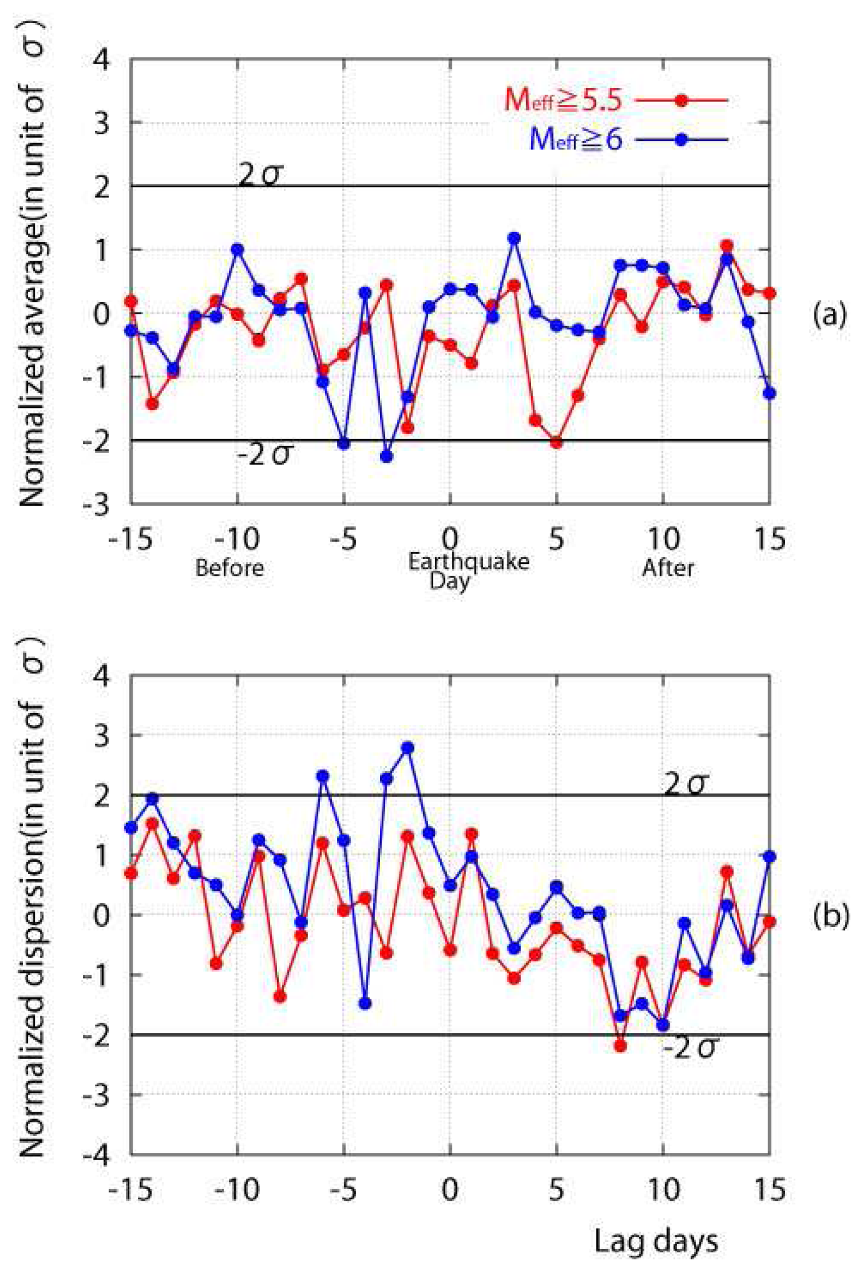
Then, we are ready to undertake a superimposed epoch analysis. For the study on the correlation between ionospheric perturbations in terms of two parameters (amplitude and dispersion) and seismicity, we choose two characteristics periods; seismically active periods with Meff greater than 5.5 and greater than 6.0. The number of events with Meff ≥ 5.5 is 19, and that with Meff ≥ 6.0 is 4.
We finally undertake the statistical test. When we perform the Fisher's z-transformation to the data amplitude and dispersion, respectively, the z value is known to follow approximately the normal distribution of N (0, 1) with zero average and dispersion of unity.
Figs. 4(a) and 4(b) represent the corresponding statistical z-test result. The 2σ (σ: standard deviation over the whole period of five years) line is indicated as the statistical criterion. First of all, we look at the amplitude (trend) result in
Fig. 4(a). It is clear that the blue line for the Meff greater than 6.0 exceeds the 2σ line (about 3 dB decrease) a few days before the earthquake. This suggests that the ionospheric perturbation in terms of amplitude (trend) shows a statistically significant precursory behavior (3 to 5 days before the earthquake). Next we go to
Fig 4(b) for the dispersion. The enhancement of dispersion (fluctuation) is clearly visible for extremely high seismic activity (Meff ≥ 6.0). That is, the dispersion is found to exceed the 2σ line 6-2 days before the earthquake day. When the Meff becomes a little smaller (Meff ≥ 5.5), the effect of earthquakes is found to be present, but it is not so significant as compared with the case for Meff ≥ 6.0. Finally, we comment on the corresponding result for M ≥ 5.0 (further below Meff = 5.5 by 0.5). We have found that the variations in amplitude and dispersion, are well inside the ±2σ line for Meff ≥ 5.0, and together with our previous findings, we say that the seismic effect can only be seen definitely for Meff ≥ 6.0.
We compare our present statistical result with previous ones (
Shvets et al., 2002;
Rozhnoi et al., 2004).
Rozhnoi et al. (2004) have studied the percentage occurrence of anomalous days for different conventional earthquake magnitudes. After examing different effects (solar flares, geomagnetic storms etc.), they have succeeded in detecting the seismic effect in subionospheric VLF/LF propagation only when the earthquake magnitude exceeds 5.5. In our analysis, we do not pay attention to the percentage occurrence of anomalous days as studied by
Rozhnoi et al. (2004), but we pay attention to two physical parameters of subionospheric LF propagation ((1) amplitude (trend) and (2) dispersion (or fluctuation)). Our result seems to have confirmed and supported our previous result by
Rozhnoi et al. (2004) by using the much longer-period data. The present statistical study has given to strong validation of the use of nighttime fluctuation method to find out seismo-ionospheric perturbations (
Hayakawa et al., 2006;
Horie et al., 2007a)
3.2. Case study of Sumatra earthquake in December, 2004 (Ground-based VLF reception in Japan) and a satellite observation of VLF signals)
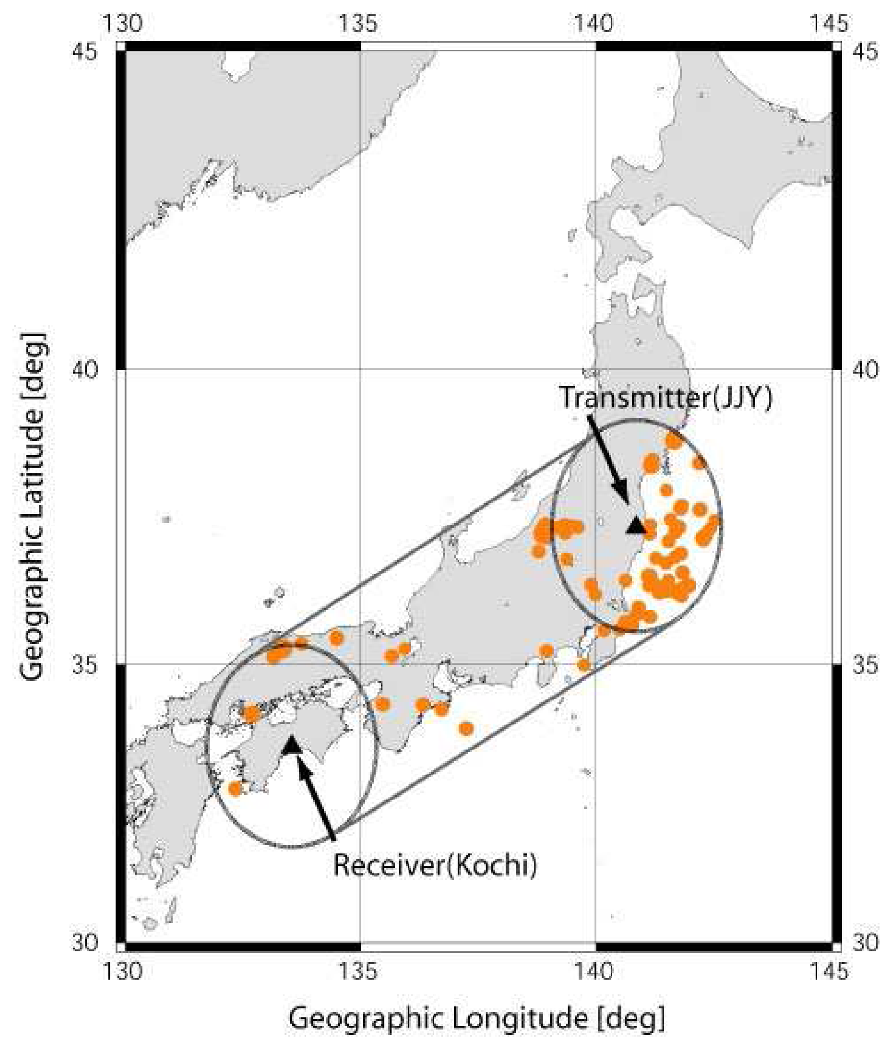
This section is concerned with a case study for the Sumatra earthquake by means of the VLF data on the propagation between the NWC VLF transmitter (Australia) (21.82 °S, 114.15 °E) to Japan. Because this earthquake is extremely huge, it is worthwhile to study whether this earthquake has a certain effect on the lower ionosphere. If the effect exists, we would like to study the characteristics and dynamics of those perturbations.
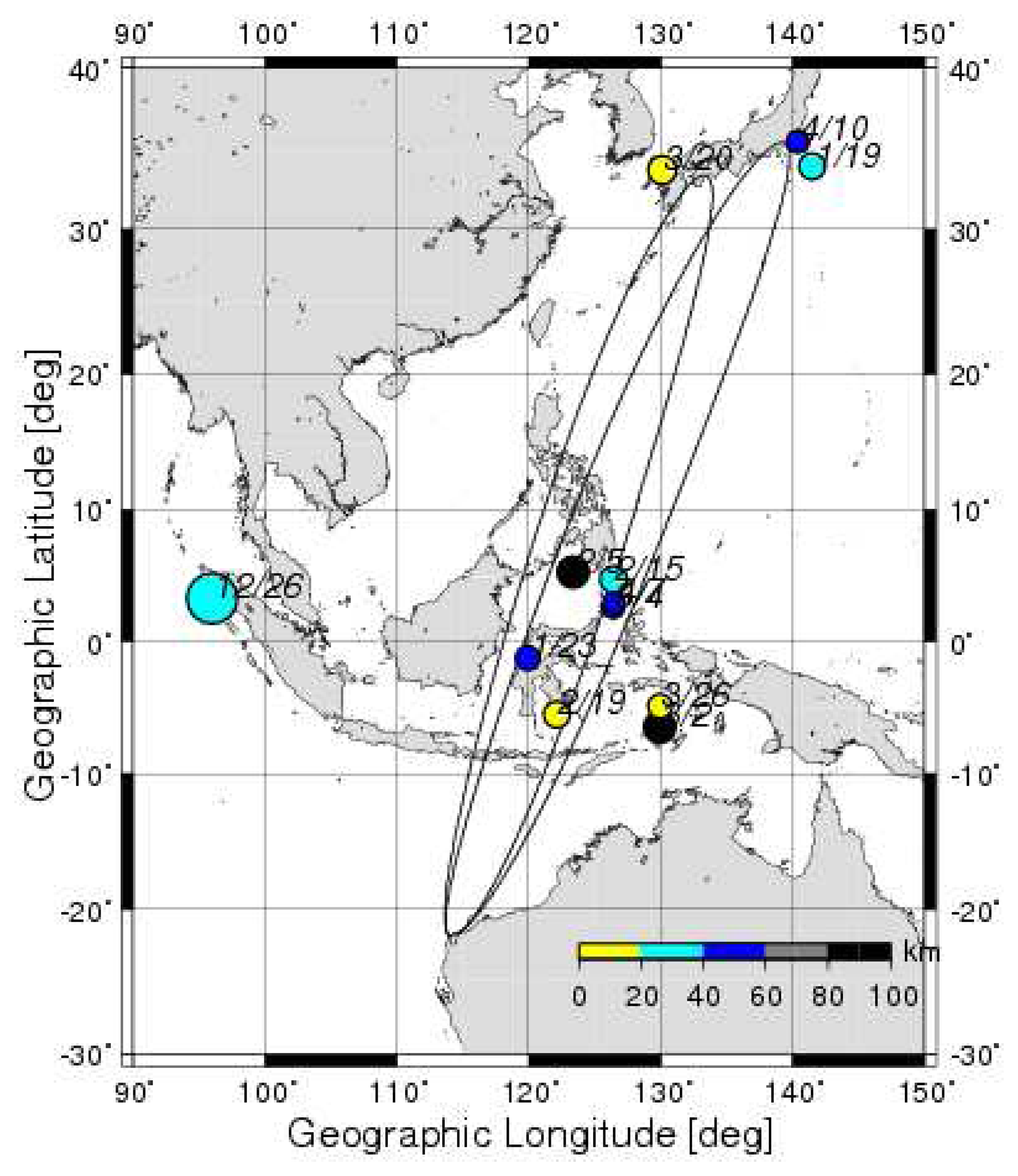
A huge earthquake happened to take place in the west coast of the Sumatra islands on 26 December, 2004. The magnitude of this earthquake is 9.3 and the focal depth is 30 km. The epicenter is located at the geographic coordinates (3.31 °N, 95.95 °E). As shown in
Fig. 5, the epicenter of this earthquake is located as a large circle (12/26), which is found to be far away (about 2,000 km) from the great-circle paths from the NWC VLF transmitter (also shown in
Fig. 5) and three Japanese receiving points (Chiba (abbreviated as CBA), Chofu (CHO) and Kochi (KOC)). The details of this VLF/LF network in Japan are given in
Hayakawa et al. (2004a,
b).
We pay particular attention to the period around the Sumatra earthquake; that is, the period from the middle of November, 2004 to May, 2005. In
Fig. 5 we have plotted only two propagation paths (two of fifth Fresnel zones for the NWC to Kochi and for the NWC to Chiba). During the period from the middle November, 2004 to May, 2005, we have indicated the epicenters of the earthquakes with magnitude greater than 6.0 and close to our propagation paths. The center of each circle indicates the epicenter of the earthquake, and its size is proportional to the magnitude. The color of the circle indicates the depth with the step of 20 km.
There have been proposed two methods of analysis to find the precursory effect of ionospheric perturbations as revealed from the VLF/LF data; (1) Terminator time method (
Hayakawa et al., 1996;
Molchanov and Hayakawa, 1998), and (2) Nighttime fluctuation analysis (
Shvets et al., 2004a,
b;
Roznoi et al., 2004;
Maekawa at al., 2006). As shown in
Fig. 5, the propagation path is approximately in the N-S meridian plane, so that the terminator time method is not so effective for this path. Because the terminator time method is effective mainly for the E-W propagation direction (
Maekawa and Hayakawa, 2006). Hence, we have adopted the fluctuation analysis.
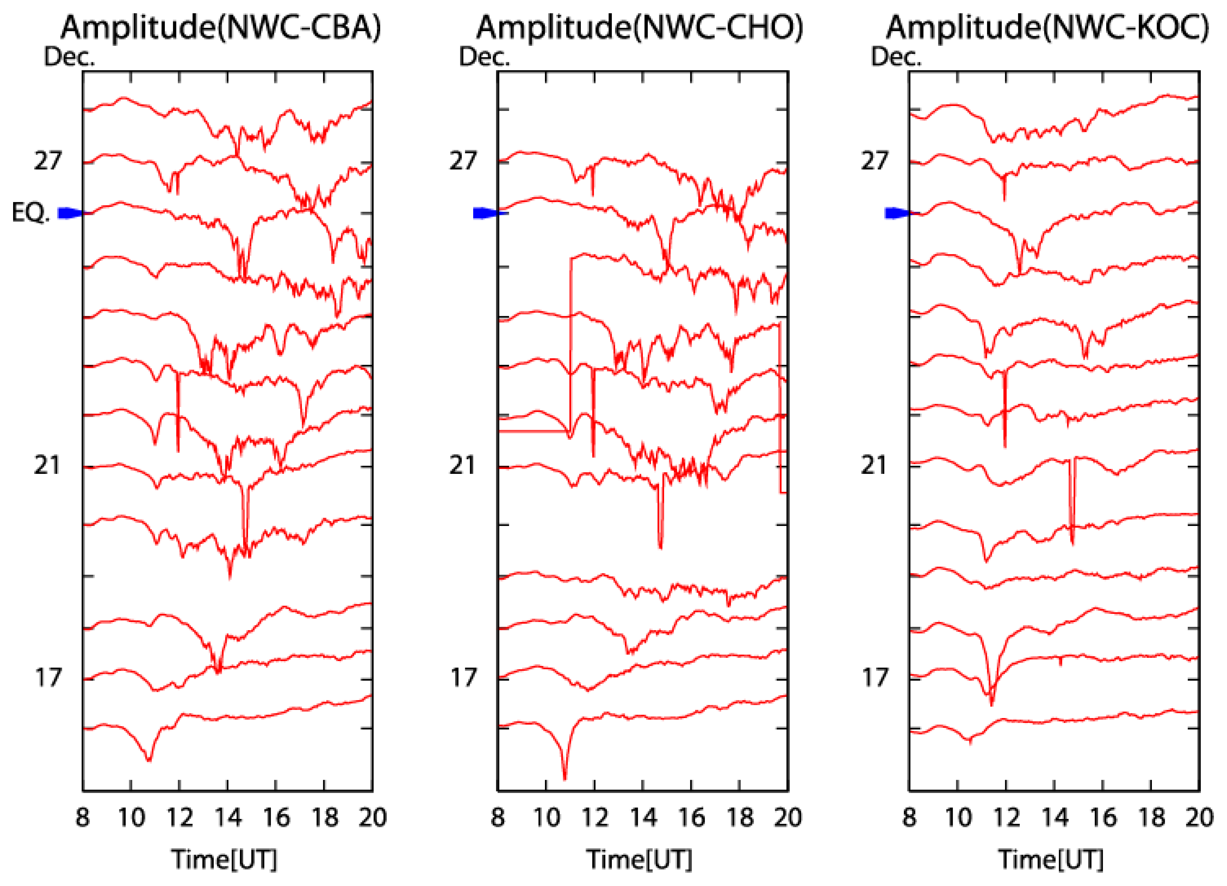
Fig. 6 is the sequential plot of nighttime amplitude of NWC signal observed at the three observing sites (Chiba (CBA), Chofu (CHO), and Kochi (KOC)). It is easy to understand qualitatively that there is an increased fluctuation in the nighttime amplitude at all the stations. Then, we will estimate this nighttime fluctuation quantitatively. We use the nighttime L.T. time internal for six hours (L.T. = 21 h to 03 h), and we estimate the difference dA(t) (≡ A(t) – <A(t)>) where A(t) is the VLF amplitude at the time t and <A(t)> is the average value over ±15 days (one month) at the same time t. Finally, we integrate dA
2 over the relevant nighttime six hours, and we have one data for each day.
As is shown in
Maekawa et al. (2006), we have shown the analysis result during the two years of 2004 and 2005. This long-term analysis was used to infer that the VLF nighttime fluctuation seems to be depleted during seismically quiet periods.
The fifth Fresnel zone shown in
Fig. 5 is already found to be useful and effective as the VLF sensitive zone for earthquakes with magnitude 6.0-7.0 (
Hayakawa et al., 1996;
Molchanov and Hayakawa, 1998), when we think of the possible size of the seismo-ionospheric perturbations. This Sumatra earthquake is extremely huge (M = 9.3), so that we expect an extremely large area of ionospheric perturbations for this earthquake. By simply using either the formula on the preparation zone size by
Dobrovolsky et al. (1979) or the empirical formula on the size of ionospheric perturbations by
Ruzhin and Depueva (1996), the radius of preparation zone or possible ionospheric perturbation is estimated to be of the order of 7,000-8,000 km. The empirical formula by
Ruzhin and Depueva (1996) is mainly based on the events mainly up to M = 7.0 or so, so that it is questionable for us to use this formula even up to M = 9.3. Even though, it may be reasonable to anticipate that the VLF propagation path from the transmitter, NWC to Japanese VLF sites is definitely influenced very much, or perturbed because the distance of the epicentre from the great-circle path is only 2,000 km.
As is already shown in
Horie et al. (2007a), the geomagnetic activity just around the Sumatra earthquake (e.g. ±one month around the earthquake) is found to be relatively quiet except just after the middle of January, 2005 when the ΣKp exceeds 40 (disturbed). For example, in December, 2004, we have found relatively quiet geomagnetic activity. We look at the VLF fluctuations just before the Sumatra earthquake. It is very fortunate that we find very prolonged seismically quiet period before the Sumatra earthquake.
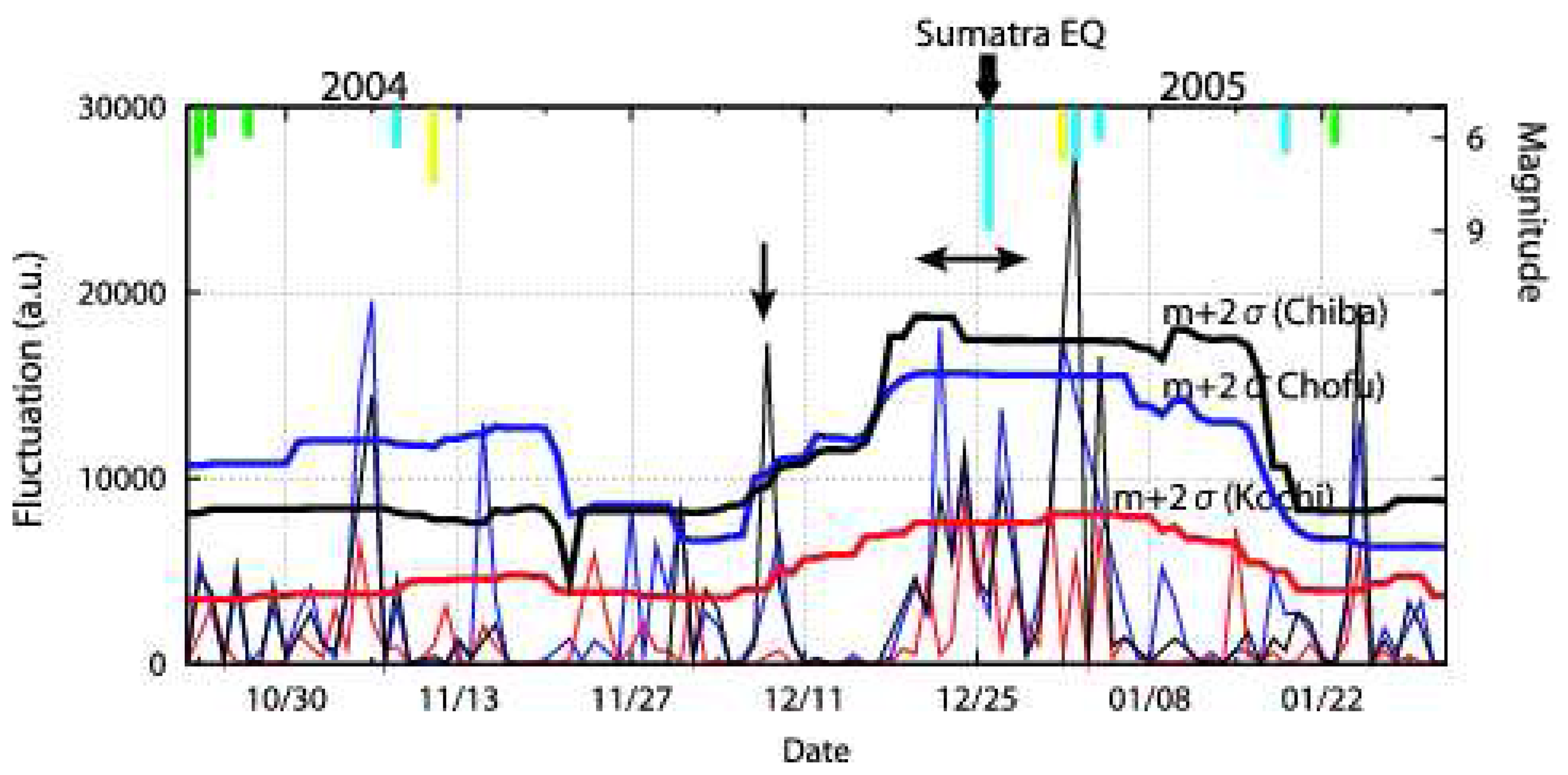
Fig. 7 is the extended figure for the limited time period just around the earthquake time. But, you see now the temporal evolutions of the nighttime fluctuation (the same integrated dA
2 over the night) at three stations (Chiba in black, Chofu in blue and Kochi in pink), together with the corresponding running value of m (mean) +2σ (standard deviation) over ±15 days (with the same color). We notice one sharp peak on 8 December, 2004 and a prolonged maximum during the period of December 21, 2004 to January 2, 2005. In the case of the fluctuation enhancement on 8 December, 2004, we notice a significant enhancement at Chiba (in black) exceeding (m + 2σ) line. However, the fluctuation at Chofu (in blue) is not found to exceed the (m + 2σ) line (given in the figure in pink) and also there is no enhancement at all at Kochi (in red). Taking into account these facts, we may conclude that the amplitude fluctuation is taking place significantly only at Chiba, which means that this enhancement on 8 December, 2004 might be the effect only for the NWC-Chiba path. Next we discuss the prolonged period of amplitude fluctuation during the period of December 21, 2004 to January 2, 2005. During this period we notice the simultaneous enhancement in fluctuations at the three observing sites (Chofu (in blue), Chiba (in black) and Kochi (in red)), which means that this prolonged fluctuation is global, and the NWC-Japan propagation path is strongly disturbed. The fluctuation at Chofu (in blue) is found to exceed significantly the (m + 2σ) line at Chofu a few days before the earthquake. Also, we recognize the similar and significant enhancement in Chiba and also in Kochi. You can notice the excess of the nighttime fluctuation over the corresponding (m + 2σ) line both at Chofu and Kochi. Even after the main shock (M = 9) on 26 December, 2004, there occurred several aftershocks on 1 ∼ 4 January, 2005 with magnitudes in a range from 6.1 to 6.7. In correspondence with this high seismic activity, there have been observed the prolonged VLF fluctuation during the period of 21 December, 2004 to 2 January, 2005.
When we look at the temporal evolutions in
Fig. 6, we can easily identify clear wave-like structures in the data. Our visual inspection could give us an idea that there exist clear wave-like structures, for example, on 16, 24 and 26 December, 2004. These structures are quantitatively investigated by means of the wavelet and cross-correlation analyses. It is expected that these fine structures like wave-like structures could provide us with the information on how the ionosphere is perturbed in association with earthquakes.
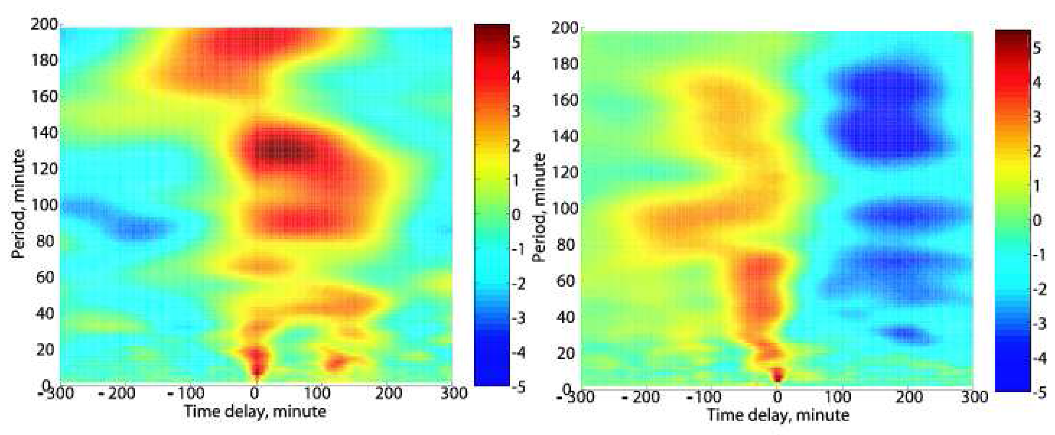
Fig. 8 is the summary of the cross-correlation analysis on the time delay of the Chiba data with respect to Kochi on the basis of superimposed epoch analysis. The left panel in
Fig. 8 corresponds to the period of 16 December to 26 December, 2004 (that is, 11 days) before the earthquake. While, the right panel is the corresponding result for the period after the earthquake (2 May to 12 May, 2005) (i.e. quite period). An important point is that the fluctuations in amplitude (dA(t)) is very enhanced in the period of 20-100 minutes before the earthquake. This epoch analysis in the left panel indicates the clear presence of time delay or wave-like structure before the earthquake. The period of fluctuation is confirmed to range from 20-30 minutes to above 100 minutes, and the time delay at the Chiba is around 2 hours with respect to Kochi. There is no significant frequency dependence (dispersion) in the time delay. The right panel of
Fig. 8 shows no such wave-like structures at all after the earthquake. So that, the presence of such wave-like structures is likely to be a precursory signature of this earthquake.
Before the earthquake, we could notice an enhancement in the fluctuation spectra in the frequency range from 20-30 minutes to about 100 minutes. This period corresponds to that of atmospheric gravity wave (AGW) (30 to 180 minutes) (
Grossard and Hooke, 1975;
Hooke, 1977) and this AGW is considered to be a possible and promising candidate for the lithosphere-ionosphere coupling (
Molchanov et al., 2001;
Miyaki et al., 2002;
Shvets et al., 2004a,
b). The wavelet at Chiba is delayed by about 2 hours with respect to that at Kochi, which is indicative of its propagating nature from the epicenter toward outsides. On the assumption that the wave is propagating radially from the epicenter, we can estimate the propagation distance between the NWC-KOC and NWC-CBA is estimated to be ∼ 150 km. So that we can estimate the wave propagation velocity of our wave-like fluctuation to be about 20 m/s. This value seems to be in good agreement with the theoretical estimation of AGWs (
Kichengast, 1996;
Hooke, 1968). The experimental evidence on the wave like fluctuations as a precursor to this Sumatra earthquake might be considered to be an evidence of the important role of AGW in the lithosphere-ionosphere coupling. Further details have appeared in
Horie et al. (2007b).
The same NWC signals have been detected on board the French satellite, DEMETER, which has indicated that the signal to noise ratio (the ratio of the VLF signal to the background noise) is found to be significantly depressed during one month before the earthquake, and that the diameter of the ionospheric perturbation as seen on the satellite is about 5,000 km (
Molchanov et al., 2006). This satellite finding on the presence of the ionospheric perturbation in association with the Sumatra earthquake and its spatial scale are found to be a further support to our ground-based VLF finding.
