Development of a Space-charge-sensing System

Hazmi, Ariadi; Takagi, Nobuyuki; Wang, Daohong; Watanabe, Teiji

doi:10.3390/s7123058

Open AccessArticle

Development of a Space-charge-sensing System

by

Ariadi Hazmi

,

Nobuyuki Takagi

,

Daohong Wang

^* and

Teiji Watanabe

Gifu University of Japan

^*

Author to whom correspondence should be addressed.

Sensors 2007, 7(12), 3058-3070; https://doi.org/10.3390/s7123058

Submission received: 21 October 2007 / Accepted: 30 November 2007 / Published: 4 December 2007

(This article belongs to the Special Issue Sensors for Disaster and Emergency Management Decision Making)

Download

Browse Figures

Versions Notes

Abstract

:

A system for remotely measuring the distribution of air space charge in real time is developed. The system consists of a loudspeaker and an electric field antenna. By propagating a burst of directional sound wave from the speaker, a modulation in the space charge and, therefore, an electric field change at ground is produced. The distribution of the space charge density is derived from the E-field change which can be measured by the E-field antenna. The developed system has been confirmed by both laboratory and field experiments.

Keywords:

Space charge; remote sensing; thundercloud; lightning

1. Introduction

Conventionally, space charge in atmosphere is either measured directly at some local preset points or inferred from measurement of potential difference through balloons, rockets or airplanes [e.g., Bradley, 1968; Winn and Moore, 1971; Chauzy et al., 1991]. The latter has been widely used for measuring the charge distribution both inside and beneath a thundercloud and has provided a lot of valuable information on electrical structure of thunderclouds [e.g., Soula and Chauzy, 1991; Marshall and Rust, 1993]. However, all conventional methods are very poor in terms of spatial resolution and they are in principle not suitable for measuring air space charge distribution in real time and in 3-dimensions. Real-time and 3-D information on the charge distribution inside a thundercloud can not only provide a direct means for forecasting imminent lightning but also help to understand thundercloud electrification mechanism and lightning discharge characteristics. We have proposed a method which is suitable for real time and 3-D measurement of space charge distribution in atmosphere [Wang et al., 1997]. In this method, a burst of directional sound wave is used to modulate the space charge and to produce an oscillating electric field which is measurable at the ground. The space charge location is determined with the time difference between the sound wave and the E-field variation in combination with the sound wave propagation direction. The space charge amplitude is derived with the amplitude of the E-field variation. The possibility of measuring atmospheric space charge by use of sound waves has been suggested by Siscoe [1971] more than 30 years ago. In his method, a continuous plane sound wave was used and the local oscillating electric fields at the space charge location had to be measured. To get some spatial resolution, either numerous measuring systems are needed or the measuring system has to be moved within air space charge region. Compared to conventional methods, his method in principle has the similar limitation in terms of spatial resolution. Our method is based on remote sensing and is capable of measuring space charge in real time and 3 dimensions with only a single stationary system. To evaluate the validity of our proposed method, in the present study a prototype of system for measuring space charge has been developed and tested in both laboratory and field conditions. This paper reports the results.

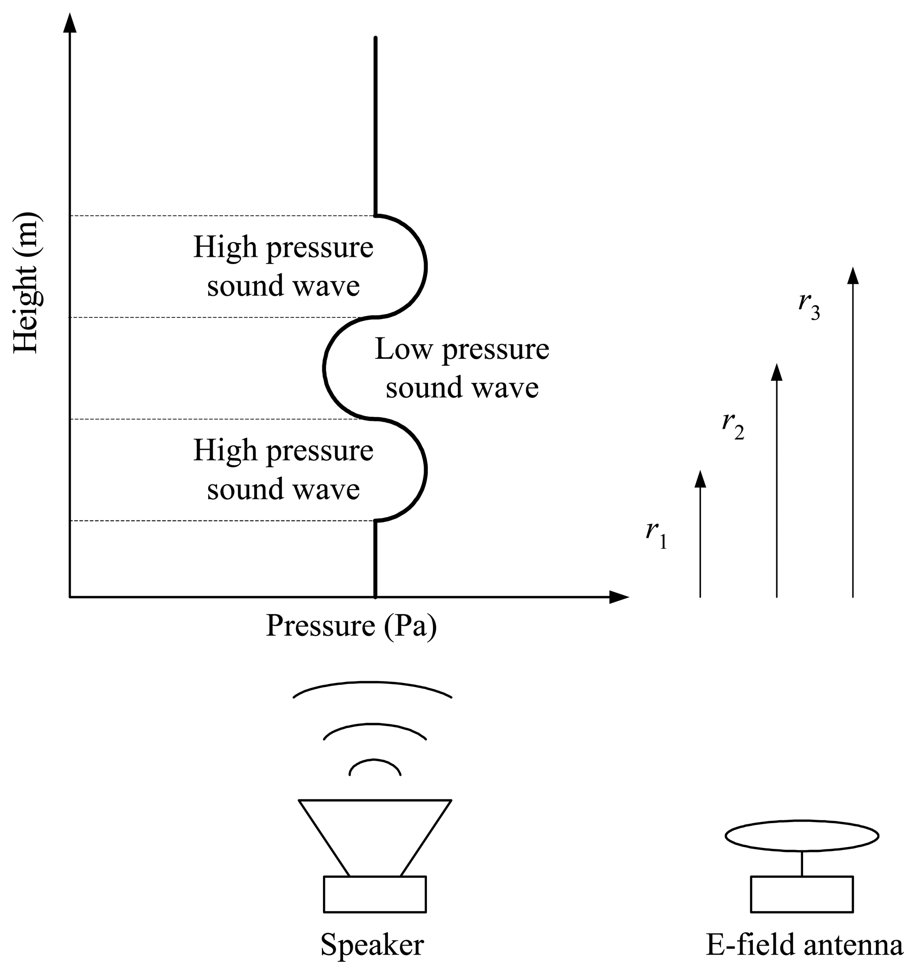
2. Theoretical Background

When a burst of directional sound wave propagates in air as shown in Fig. 1, the air density along the sound wave will be modulated in sequences by the sound wave. The air density ρ modulated at a distance of r from the loud speaker can be calculated with the following formula (see the detail in Appendix A).

ρ (r, t) = ρ_{0} [1 + \frac{A}{γ P_{0}} \cdot e^{- α γ} \cdot e^{j (ω t - K r)}]

(1)

where ρ₀ is the air density in steady state, with value of ρ₀ = 1.293 kg m^-3; A is the amplitude of sound wave (Pa); γ is the ratio of the specific heat at constant pressure to the specific heat at constant volume, with value of γ = 1.402; P₀ is the atmospheric pressure in steady state, with value of P₀ = 1.013×10⁵ Pa; α is the attenuation constant; ω is the angular frequency of the sound wave; K is wave number where K = ω/c, c is the sound velocity. If the space charge density ρ_e is in proportion to ρ, which should be true for most of cases, the space charge density is modulated similarly as the air density. The modulation in ρ_e can produce an oscillating electric field changes at ground. Assume that the sound wave lasts 1.5 periods (or 1.5 wavelengths), the following relation can be easily derived (see the detail in Appendix A).

E = \frac{1}{ε_{0} γ P_{0}} \frac{ρ_{e 0} sin θ}{f r} \sqrt{\frac{ρ_{0} c^{3}}{8 π^{3}} W}

(2)

where E is the amplitude of the electric field change; ε₀ is the dielectric constant in vacuum; f is the frequency of the sound wave; r is the propagation distance of the sound wave; θ is the half angle of the directional sound wave; c is the speed of sound; W is the input power into the speaker. By measuring E, the space charge density along the propagation of sound wave could be derived with the above formula. By changing the direction and frequency of the sound wave, it is possible to obtain 3-dimensional space charge distributions in a similar way to typical meteorological radar.

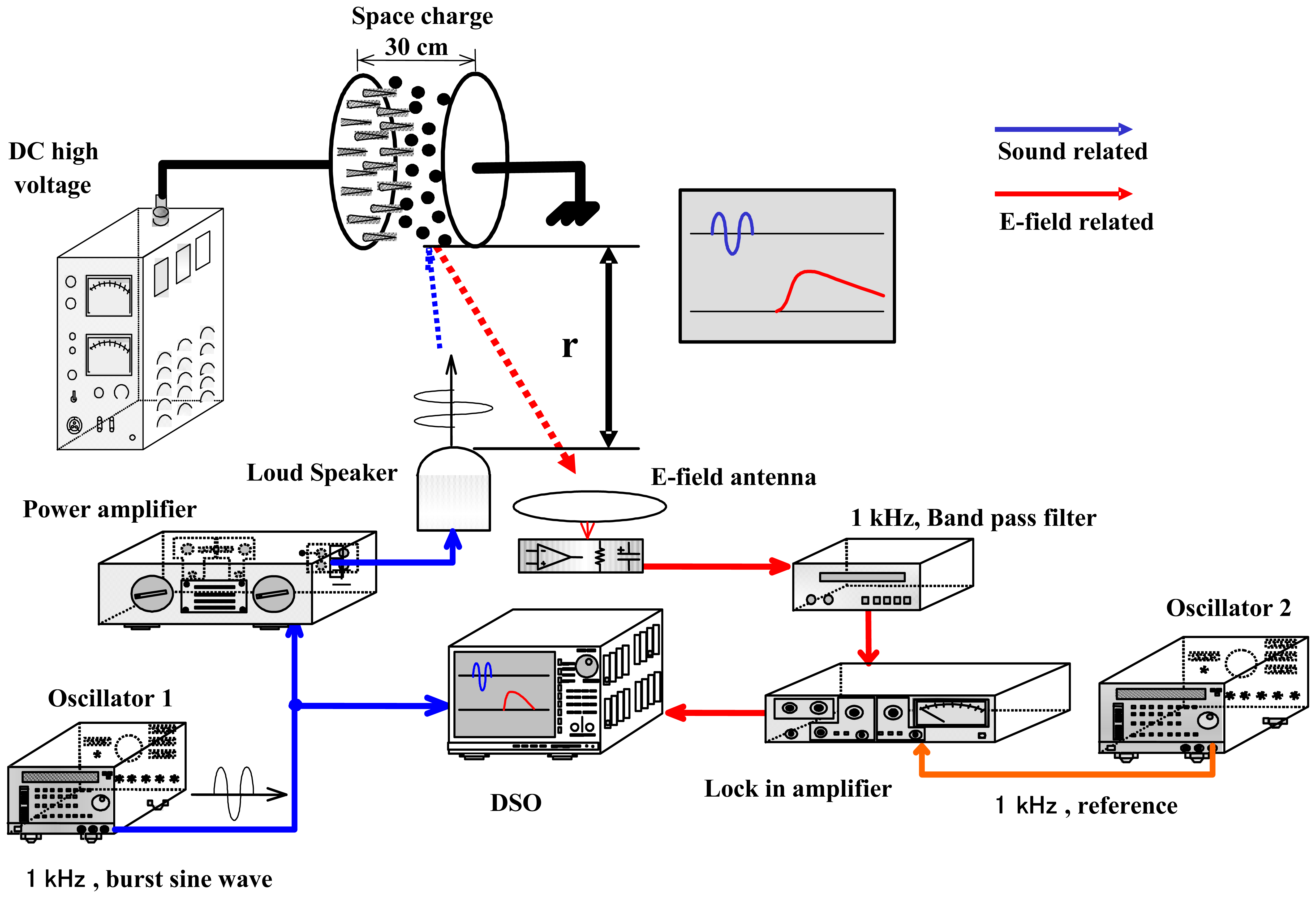
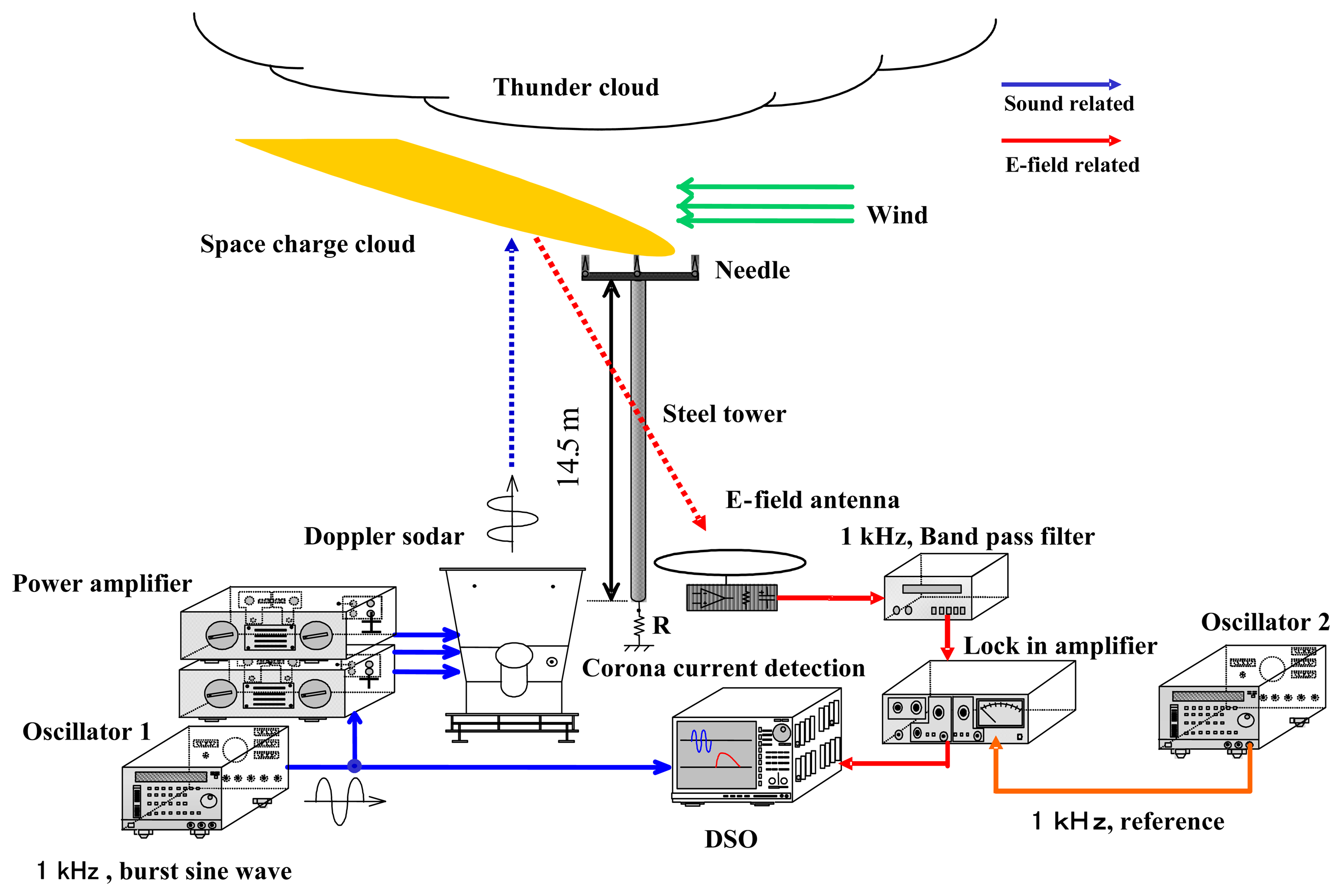
3. Experimental Set-up

The diagram of the developed system and also the set-up for laboratory experiments are shown in Fig. 2. The experiment set-up consists of three parts: (1) space charge producing part, (2) sound wave generating part and (3) electric field measuring part. As illustrated in Fig. 2, the space charge producing part is composed of a DC high voltage power supply and two plate electrodes with one of them having 15 short needles on its inner surface. The space charge is generated though corona discharging from the needles. The resultant charge density can be adjusted by changing the applied voltages. The sound wave generation part consists of an oscillator, a power amplifier and a loudspeaker. The oscillator outputs a burst sine wave with 1 kHz frequency and 1.5 wavelengths every second. The electric field measuring part is composed of a capacitive electric field antenna, a band-pass filter, a lock-in amplifier and a digital storage oscilloscope. The lock-in amplifier is used to reduce noise and to improve the sensitivity of the E-field measuring system. The output of the lock-in amplifier takes the form of integration of the E-field variation.

The set-up of field experiments is shown in Fig. 3. In field experiments, the space charge is produced under thunderstorm conditions through corona discharges occurred from several needles which are mounted on the top of a 14.5 m high grounded tower. In order to measure the space charge in field environments, a powerful loudspeaker for Doppler sodar as specified in Table 1, is used. All the other equipments used in field are the same to that in laboratory and have already been described above.

4. Results

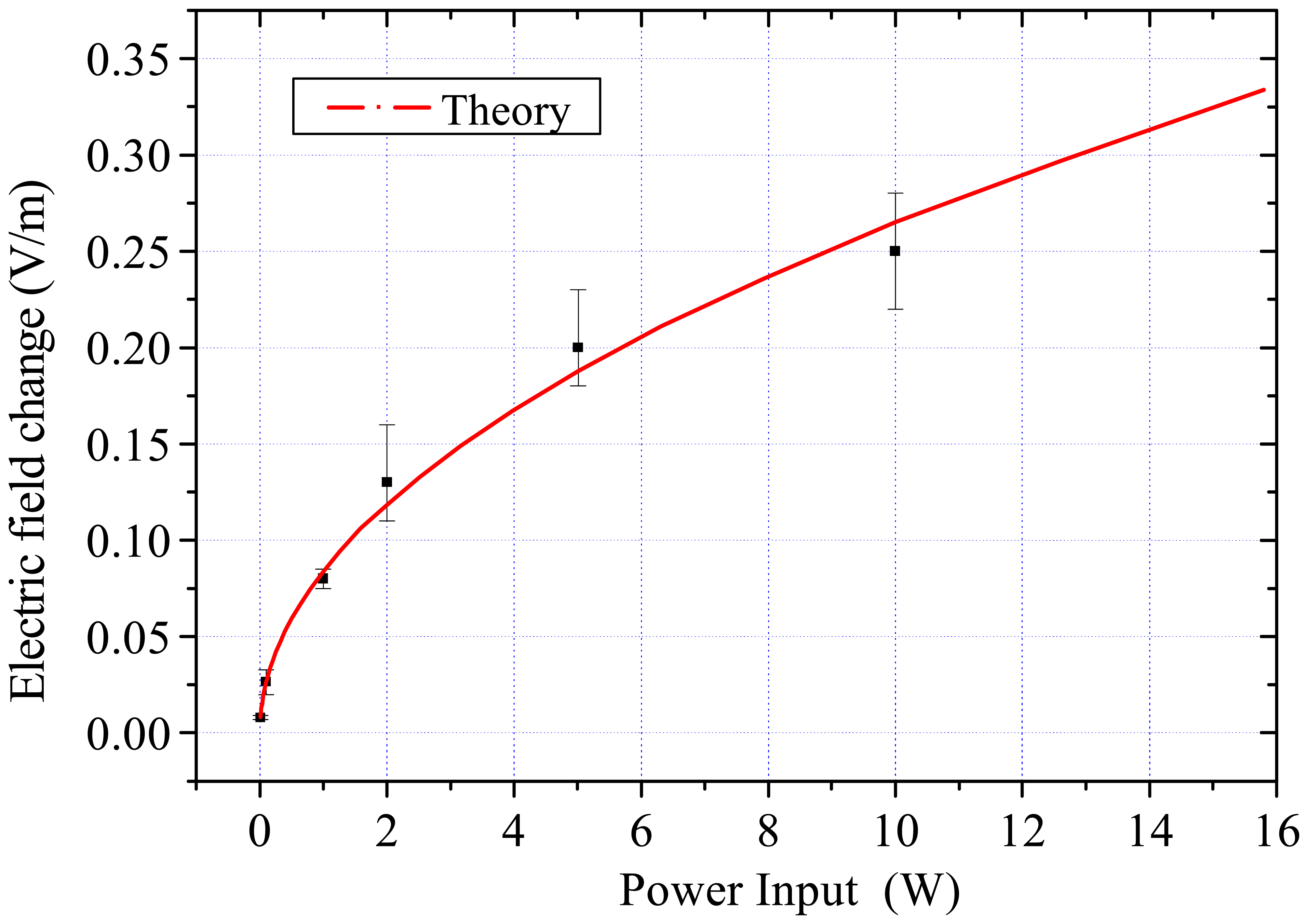
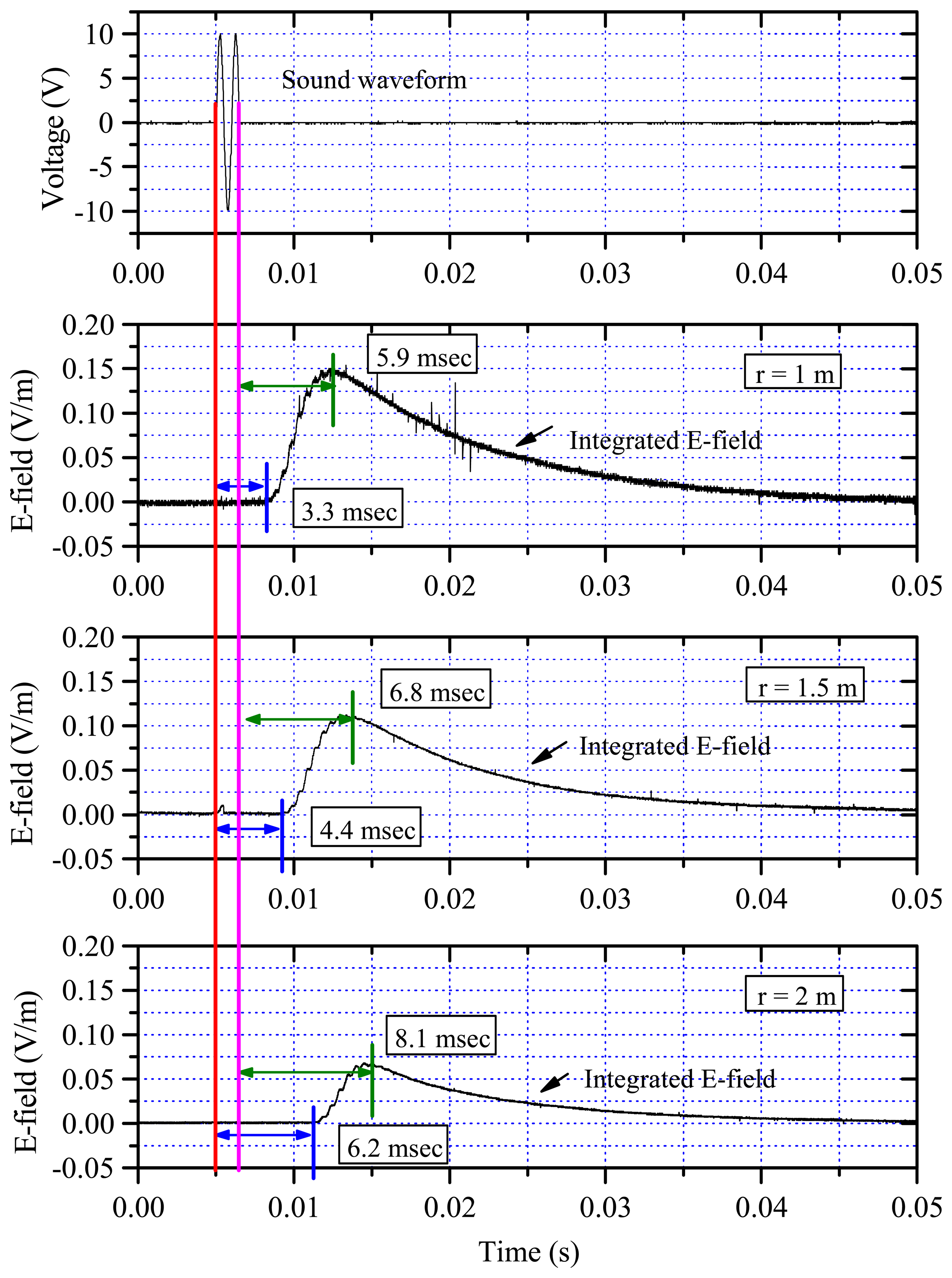
4.1 Results obtained in laboratory experiments

Fig. 4 shows an example of the burst sound wave and the integrated electric field changes when the distances between the loud speaker and the bottom of the electrode are, respectively, 1, 1.5 and 2 meters. In the E-field waveforms, the beginning time of the E-field rise and its peak time are marked as shown in Fig. 4. The start of generating sound wave is referred as t = 0. Compared to the sound wave, since the traveling time for an electromagnetic wave can be neglected, the beginning time of E-field rise in the E-field waveforms is the propagation time for the sound wave front to arrive at the bottom of the space charge region. Multiplication of this time with the sound speed results in the distance between the speaker and the bottom boundary of the space charge. This distance, denoted r, is shown in each of the bottom three plates of Fig. 4. The peak time corresponds to the propagation time for the sound wave to leave the space charge region. Multiplication of this peak time with the sound speed results in the distance between the loud speaker and the top end of the electrodes, which is equivalent to r + 0.7 m. The distances calculated are in good agreement with the measured distances with errors less than 10%. Also as seen in Fig. 4, the shorter the separation distances between the speaker and the space charge, the larger are the peak values of the integrated electric field changes. This is also in good agreement with equation (2).

Fig. 5 shows the relationship between the detected electric field changes and the powers inputted to the loud speaker. As seen in Fig. 5, the larger the input power, the bigger is the amplitude of the electric field change. A theoretical curve predicted by equation (2) is also included in Fig. 5. The experimental data are in reasonably good agreement with the theoretical curve.

From the measured E-field changes, the charge density inside the electrodes can be derived with equation (2). Meanwhile, in order to have a comparison the space charge has been measured by other two independent methods. In the first method, referred to as voltage method in this paper, the electric field E at the inside surface of the earth plate electrode and the voltage between the two plate electrodes with distance d are measured. The space charge density can be estimated by,

ρ_{c} = \frac{2 ε_{0}}{d} (E_{0} - \frac{V}{d})

(3)

where ρ_c is space charge density; E₀ is the electric field at the inside surface of the earthed electrode; V is the voltage between the two electrodes and ε₀ is the dielectric constant in vacuum.

In the second method, referred to as corona current method in this paper, the total corona current flowing to the earth, and the electric field on the inside surface of the earthed plate are measured. The charge density ρ can be estimated by

ρ = \frac{I}{E_{0} μ S}

(4)

where I is the corona current; E₀ is the electric field between the two electrodes; μ is mobility of ion, with value of μ is 1.32×10^-4 m² s^-1 V^-1; S is the cross sectional area of the space charge. The electric field on the inside surface of the earthed electrodes was measured with a field mill. The corona current was measured through a resistor. Fig. 6 shows the space charge densities measured with three different and independent methods at various applied DC voltages. As seen in Fig. 6, the larger the applied voltage, the bigger are the space charge densities. All three methods are in good agreements.

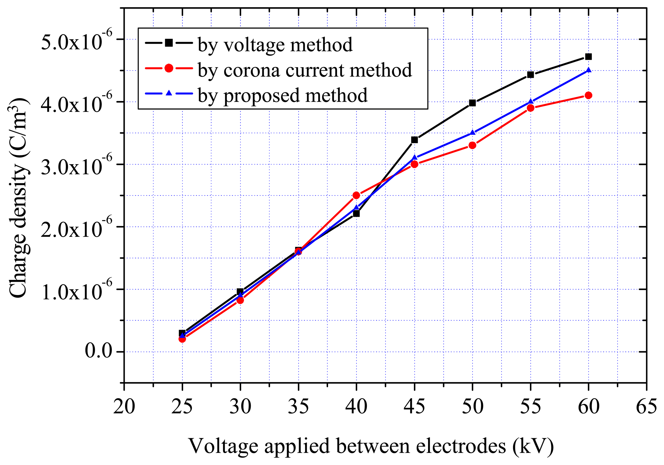
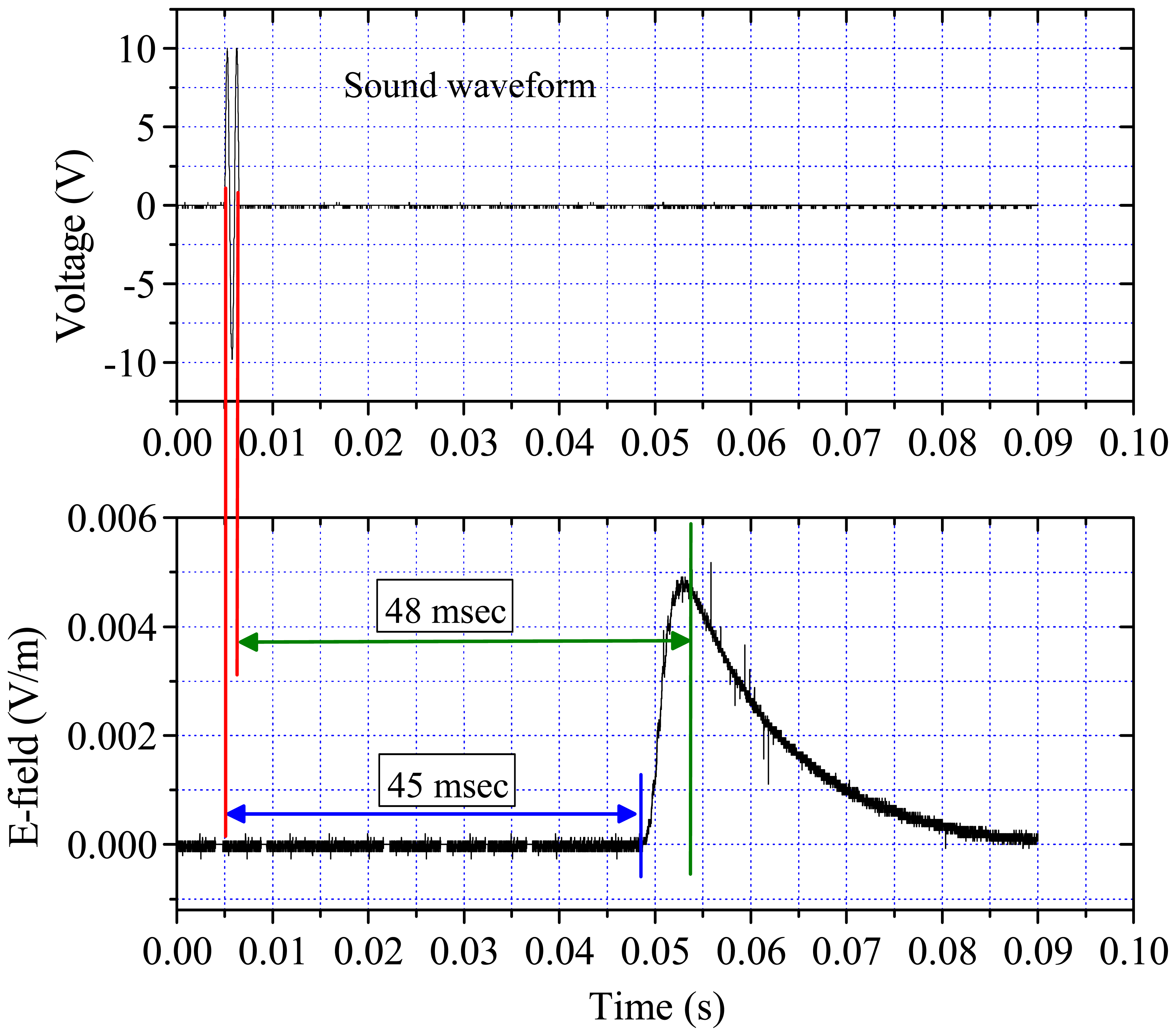
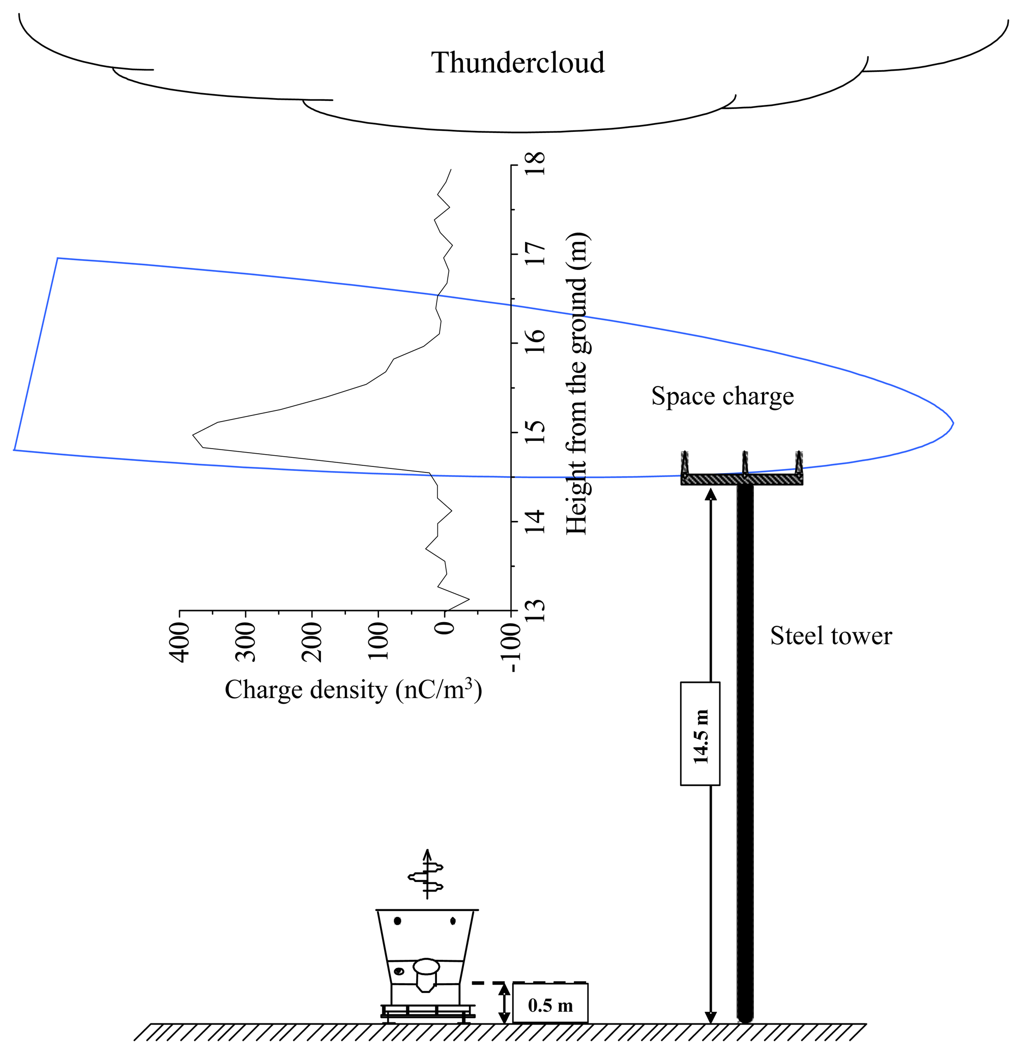
4.2 Results obtained in field experiments

Fig. 7 shows an example of the sound wave and the integrated electric field detected under a thundercloud. Based on these measured waveforms, the space charge distribution can be estimated by using equation (2). The space charges appear to exist in the region from 14.9 m to 16 m high above the ground and have maximum charge density of 400 nC m^-3 as shown in Fig. 8. The height of the charge region is consistent with the height of the grounded tower. The measured charge density is about 10 times as large as the value measured above a truck farm under the winter thundercloud [Tatsuoka et al., 1991]. The electric field on the top of 14.5 m tower is on average more than 10 times larger than that above the truck farm, and this may account for why the charge density measured by us is larger than that by Tatsuoka et al. (1991).

5. Concluding Remarks

A system for remotely measuring the distribution of air space charge in real time is developed. The system consists of a loudspeaker and an electric field antenna. The validity of the developed system has been confirmed by both laboratory and field experiments. In the future, in order to improve the sensitivity of the system, not only the noise level of the electric field antenna should be reduced, but also the output power of the loudspeaker should be increased.

Acknowledgments

The work leading to this paper is supported in part by the Ministry of Education, Culture, Sport, Science and Technology of Japan (Research Grand No. 14550262).

Appendix A Equations relating sound wave to electric field

The entire pressure P [Lauren et.al, 1982; Fahy, 1989] can be expressed as

P = P_{0} + A e^{- α γ} \cdot e^{j (ω t - K r)}

(A1)

where

P = the entire pressure (Pa)
P₀ = the atmospheric pressure in steady state (1.013×10⁵ Pa)
A = amplitude of sound pressure (Pa)
γ = the ratio of specific heat at constant pressure to constant volume (1.402)
α = the attenuation constant
ω = the angular frequency of the sound wave
K = the wave number
r = the propagation distance of the sound wave (m)

K = \frac{ω}{c} = \frac{2 π f}{c} = \frac{2 π}{λ}

(A2)

where

c = the speed of sound (331.5 m s^-1)
f = the frequency of the sound wave (Hz)
λ = wavelength (m)

\frac{P}{P_{0}} = {[\frac{ρ}{ρ_{0}}]}^{γ}

(A3)

where

ρ = the air density (kg m^-3)
ρ₀ = the air density in steady state (1.293 kg m^-3)

\frac{ρ - ρ_{0}}{ρ_{0}} ≪ 1

(A4)

{[\frac{ρ}{ρ_{0}}]}^{γ} = {[1 + \frac{ρ - ρ_{0}}{ρ_{0}}]}^{γ} = 1 + γ \frac{ρ - ρ_{0}}{ρ_{0}} = \frac{P}{P_{0}}

∴ ρ = ρ_{0} [1 + \frac{P - P_{0}}{γ P_{0}}]

(A5)

ρ (r, t) = ρ_{0} [1 + \frac{A}{γ P_{0}} \cdot e^{- α γ} \cdot e^{j (ω t - K r)}]

(A6)

The space charge density ρ_e is in proportion to ρ, which should be true for most of cases; the space charge density ρ_e is modulated similarly as the air density.

ρ_{e} = (r, t) = ρ_{e 0} [1 + \frac{A}{γ P_{0}} \cdot e^{- α γ} \cdot e^{j (ω t - K r)}]

(A7)

where

ρ_e = space charge density (C m^-3)
ρ_e0 = space charge density in steady state (1 nC m^-3)
A = amplitude of sound pressure (Pa)

In air, it is plausible to assume α is zero. The actual sound pressure is the real part of (A7),

ρ_{e} (r, t) = ρ_{e 0} [1 + \frac{A}{γ P_{0}} cos (ω t - K r)]

(A8)

On the other hand, the electric field caused by the space charge shown in Fig.A1 in spherical coordinate is

E' = \int \int \int \frac{ρ_{e} d V}{4 π ε_{0} r^{2}}

(A9)

d V = d r \cdot r d λ \cdot r sin λ d ϕ

E' = \int_{r_{2}}^{r_{1}} \int_{0}^{θ} \int_{0}^{2 π} \frac{ρ_{e} (r, t) cos λ}{4 π ε_{0} r^{2}} \cdot r^{2} sin λ d ϕ d θ d r

(A10)

\begin{array}{l} = \int_{r_{2}}^{r_{1}} \int_{0}^{θ} \frac{ρ_{e} (r, t)}{2 ε_{0}} cos λ \cdot sin λ d θ d r \\ = \frac{{sin}^{2} θ}{4 ε_{0}} \int_{r_{2}}^{r_{1}} ρ_{e} (r, t) d r \end{array}

= \frac{{sin}^{2} θ}{4 ε_{0}} ρ_{e 0} [(r_{2} - r_{1}) - \frac{A}{γ P_{0} K} {sin (ω t - K r_{2}) - sin (ω t - K r_{1})}]

(A11)

From (A11), electric field change ΔE is

Δ E = \frac{{sin}^{2} θ}{4 ε_{0}} \cdot ρ_{e 0} \cdot \frac{A}{γ P_{0} K} {sin (ω t - K r_{1}) - sin (ω t - K r_{2})}

(A12)

= 2 {\frac{{sin}^{2} θ}{4 ε_{0}} \cdot ρ_{e 0} \cdot \frac{A}{γ P_{0} K}} \cdot sin \frac{K}{2} (r_{2} - r_{1}) \cdot cos {ω t - \frac{K}{2} (r_{2} + r_{1})}

)

(A13)

From (A13), amplitude of electric field change is

E = 2 {\frac{{sin}^{2} θ}{4 ε_{0}} \cdot ρ_{e 0} \cdot \frac{A}{γ P_{0} K}} \cdot sin \frac{K}{2} (r_{2} - r_{1})

(A14)

\begin{matrix} (r_{2} - r_{1}) = n λ + \frac{λ}{2} & (n = 1, 2, \dots) \end{matrix}

(A15)

The sound power from sound source is

W = S \cdot I = π {sin}^{2} θ r^{2} \cdot \frac{A^{2}}{2 ρ_{0} c}

(A16)

where

W = the sound power (Watt)
S = area (m²)
I = the sound intensity (Watt m^-2)

The sound pressure A is eliminated from equations (A14) - (A16), the amplitude of electric field change can be derived as follows

E = \frac{1}{ε_{0} γ P_{0}} \frac{ρ_{e 0} sin θ}{f r} \sqrt{\frac{ρ_{0} c^{3}}{8 π^{3}} W} .

(A17)

Figure A1. An illustration of propagation of the sound wave to the sky.

References

Bradley, W. E. Aircraft soundings of potential gradient, space charge and conduction current, and their relation to precipitation. J. Atmospheric Sciences 1968, 25, 863–870. [Google Scholar]
Chauzy, S.; Medale, J. C.; Prieur, S.; Soula, S. Multilevel measurements of the electric field underneath a thundercloud, 1. A new system and the associated data processing. J. Geophys. Res. 1991, 96(D12), 22319–223326. [Google Scholar]
Fahy, F. J. Sound Intensity; Elsevier Applied Science: London, U.K., 1989. [Google Scholar]
Lauren, E. K.; Austin, R. F.; Alan, B. C.; James, V. S. Fundamentals of acoustics; John Willey & Sons: New York, 1982. [Google Scholar]
Siscoe, G. L. On the possibility of measuring atmospheric space charge by use of sound waves. J. Geophys. Res. 1971, 76(18), 4153–4159. [Google Scholar]
Soula, S.; Chauzy, S. Multilevel measurements of the electric field underneath a thundercloud, 2. Dynamical evolution of a ground space charge layer. J. Geophys. Res. 1991, 96(D12), 22327–22336. [Google Scholar]
Marshall, T. C.; Rust, W. D. Two types of vertical electrical structures in stratiform precipitation regions of mesoscale convective systems. Bull. American Meteor. Soc. 1993, 74, 2159–2170. [Google Scholar]
Tatsuoka, K. Electric field measurement by rocket under the thunderclouds. Proceedings of the 7th International Symposium on High Voltage Engineering, Dresden, Germany, Aug 26-30, 1991.
Wang, D.; Morisita, S.; Yoshihasi, H.; Chen, M.; Takagi, N.; Watanabe, T. Remote sensing of space charge distribution with sound wave and radio wave. National Convention of the IEE Japan 1997. Paper No. 1728. [Google Scholar]
Winn, W. P.; Moore, C. B. Electric field measurements in thunderclouds. J. Geophys. Res. 1971, 76(21), 5003–5071. [Google Scholar]

Figure 1. A schematic illustration of the principle of the developed system.

Figure 2. A schematic illustration of the setup for measuring space charge in laboratory.

Figure 3. A schematic illustration of field experiment setup for measuring space charge generated from needles on the top of a steel tower.

Figure 4. Integrated E-fields at various separation distances between space charge and the loudspeaker.

Figure 5. Relationship between the E-field changes and the power inputted.

Figure 6. Comparison of the space charge densities measured with three independent

Figure 7. Integrated E-field detected under a thundercloud.

Figure 8. An example result measured in field with the developed system

Table1. Specification of Doppler Sodar AT-900.

**Table1.** Specification of Doppler Sodar AT-900.
Frequency band	150 – 6000 Hz
Beam width	16°
Input power	900 W
Drive impedance	4Ω
Height	2.1 m

Share and Cite

MDPI and ACS Style

Hazmi, A.; Takagi, N.; Wang, D.; Watanabe, T. Development of a Space-charge-sensing System. Sensors 2007, 7, 3058-3070. https://doi.org/10.3390/s7123058

AMA Style

Hazmi A, Takagi N, Wang D, Watanabe T. Development of a Space-charge-sensing System. Sensors. 2007; 7(12):3058-3070. https://doi.org/10.3390/s7123058

Chicago/Turabian Style

Hazmi, Ariadi, Nobuyuki Takagi, Daohong Wang, and Teiji Watanabe. 2007. "Development of a Space-charge-sensing System" Sensors 7, no. 12: 3058-3070. https://doi.org/10.3390/s7123058

Article Menu

Development of a Space-charge-sensing System

Abstract

1. Introduction

2. Theoretical Background

3. Experimental Set-up

4. Results

4.1 Results obtained in laboratory experiments

4.2 Results obtained in field experiments

5. Concluding Remarks

Acknowledgments

Appendix A Equations relating sound wave to electric field

References

Share and Cite

Article Metrics

Article Access Statistics

Further Information

Guidelines

MDPI Initiatives

Follow MDPI