
Derivation of the Cramér-Rao Bound in the GNSS-Reflectometry Context for Static, Ground-Based Receivers in Scenarios with Coherent Reflection

Abstract
:1. Introduction
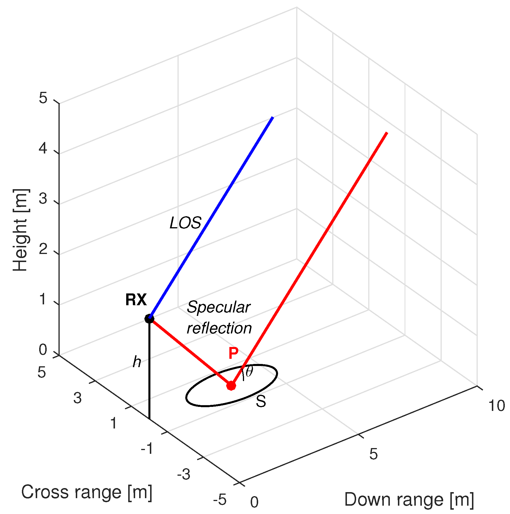
2. Scenario Definition
Signal Model at the Output of the Receiver Front-End
3. Derivation of the CRB for Short Observation Intervals
3.1. Definition and General Case for M Propagation Paths
3.2. Two Propagation Path Case for a Ground-Based Static Receiver
3.3. Introducing Phase Coherence Using FIM’s Parameter Transformation
4. Analysis of the CRB for Short Observation Intervals
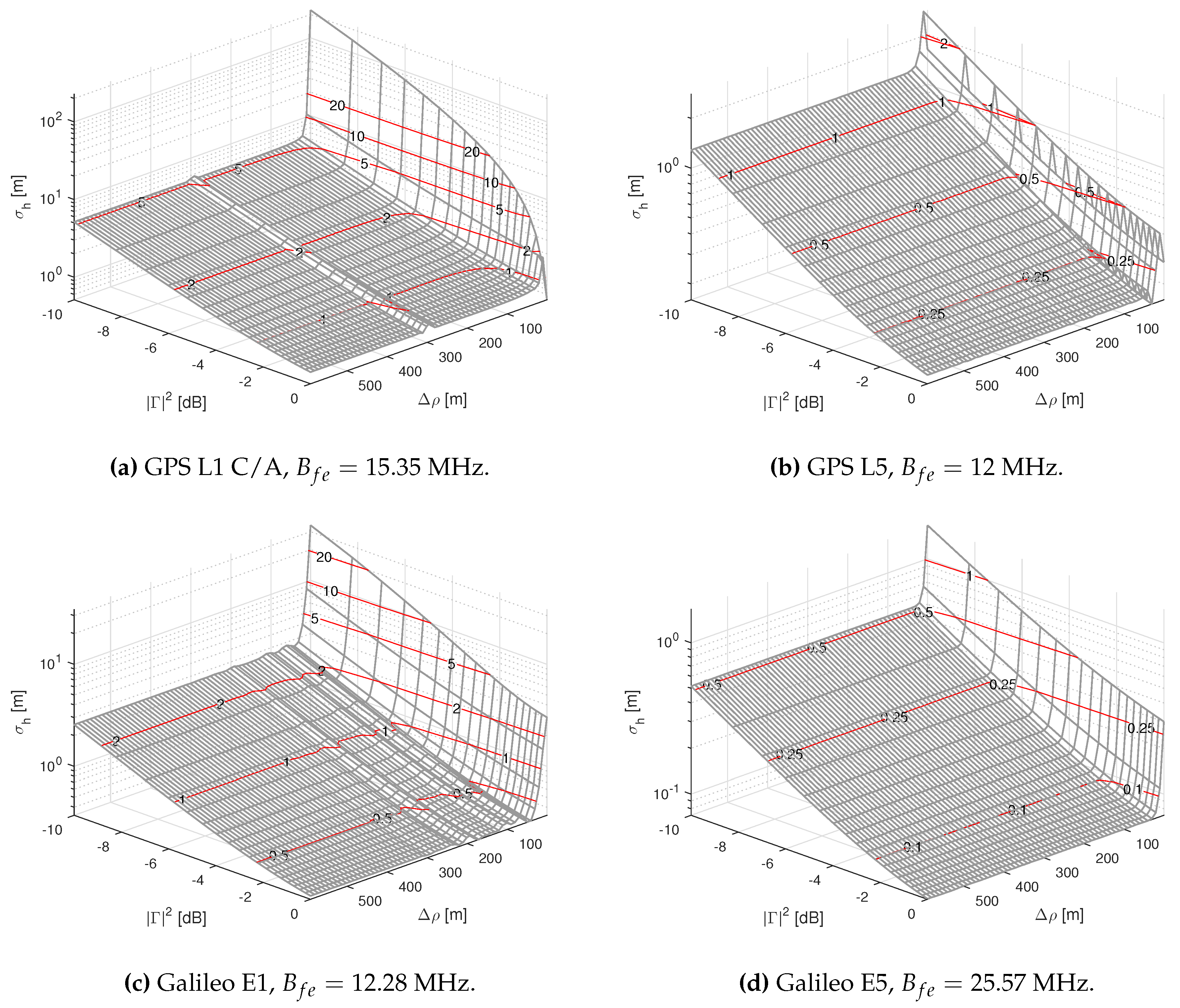
- i
- The scenario geometry: through the propagation path difference between the two signal components , which will be a function of h and the satellite elevation angle (and its variation) during the observation time.
- ii
- The properties of the reflecting surface: through its reflection coefficient, Γ, that can be modeled as a function of the signal’s incident angle and the electrical properties of the surface and its roughness.
- iii
- The GNSS signal considered and the receiver features: the signal modulation and its transmission bandwidth, the C/N0 of the LOS signal, the antenna’s radiation pattern and the receiver front-end’s bandwidth (and the filtering scheme considered) will all have an impact on the resulting CRB.
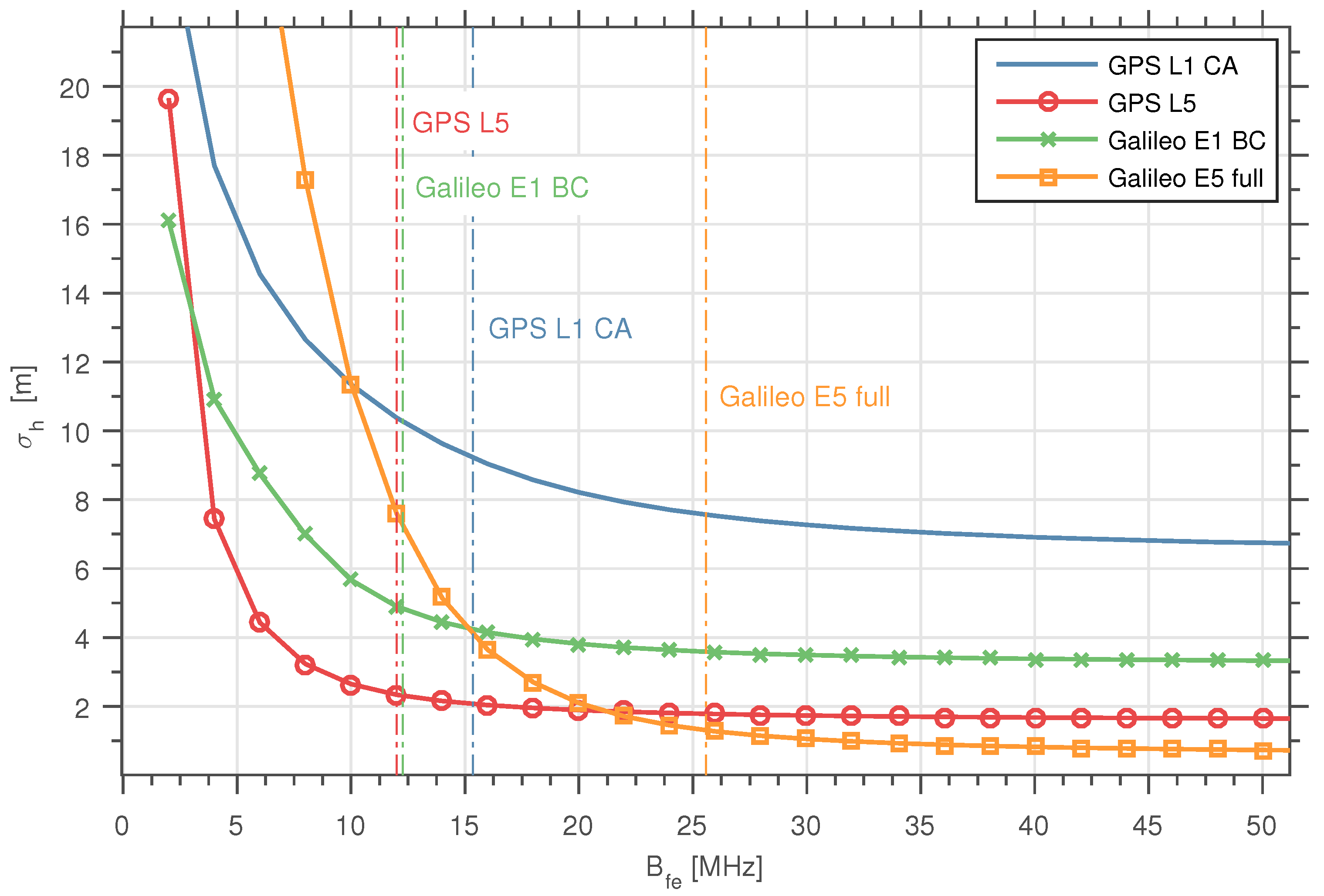
4.1. CRB when
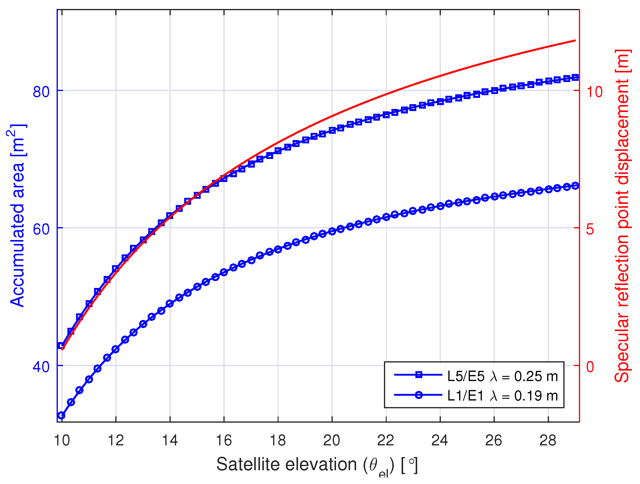
- With little surprise, both CRB expressions are inversely proportional to SNR0. However, is also inversely proportional to . This poses a trade-off: we require low elevations for the smooth surface assumption to hold, but at the same time, the lower the elevation, the higher the . Moreover, as shown by Equation (2), low elevation angles imply larger first Fresnel zone areas, which decrease the spatial resolution of our estimates.
- The values that can take for different values are bounded, as a consequence of having defined Γ as a ratio, with .
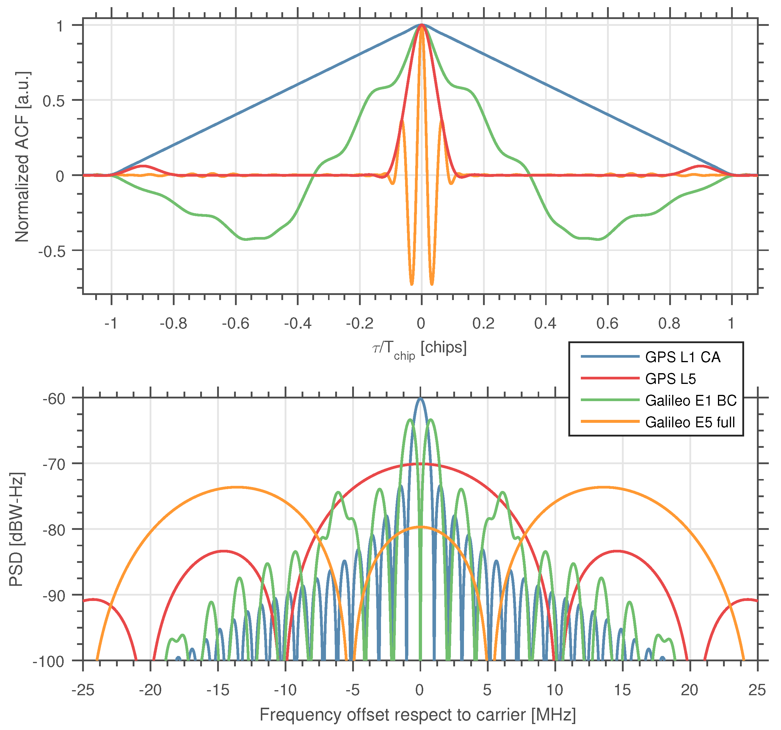
- In both CRB expressions, the effects of the assumed received signal bandwidth and the front-end filtering (possible losses and distortions) are modeled within the and the ACF’s peak, i.e., . can be understood as the curvature or the sharpness of the . The higher the front-end bandwidth, the sharper the resulting ACF peak and, thus, the higher . This holds as long as the front-end bandwidth is narrower than the received signal bandwidth, otherwise there will be no sharpening on the resulting . Additionally, for a higher front-end bandwidth, the will also increase if the Nyquist sampling rate assumption is maintained, as a consequence of having more samples for the same .
4.1.1. Phase Altimetry
4.1.2. Reflection Coefficient Estimation
4.2. CRB when : Interference Case
5. Derivation of the CRB for Long Observation Intervals: CRB()
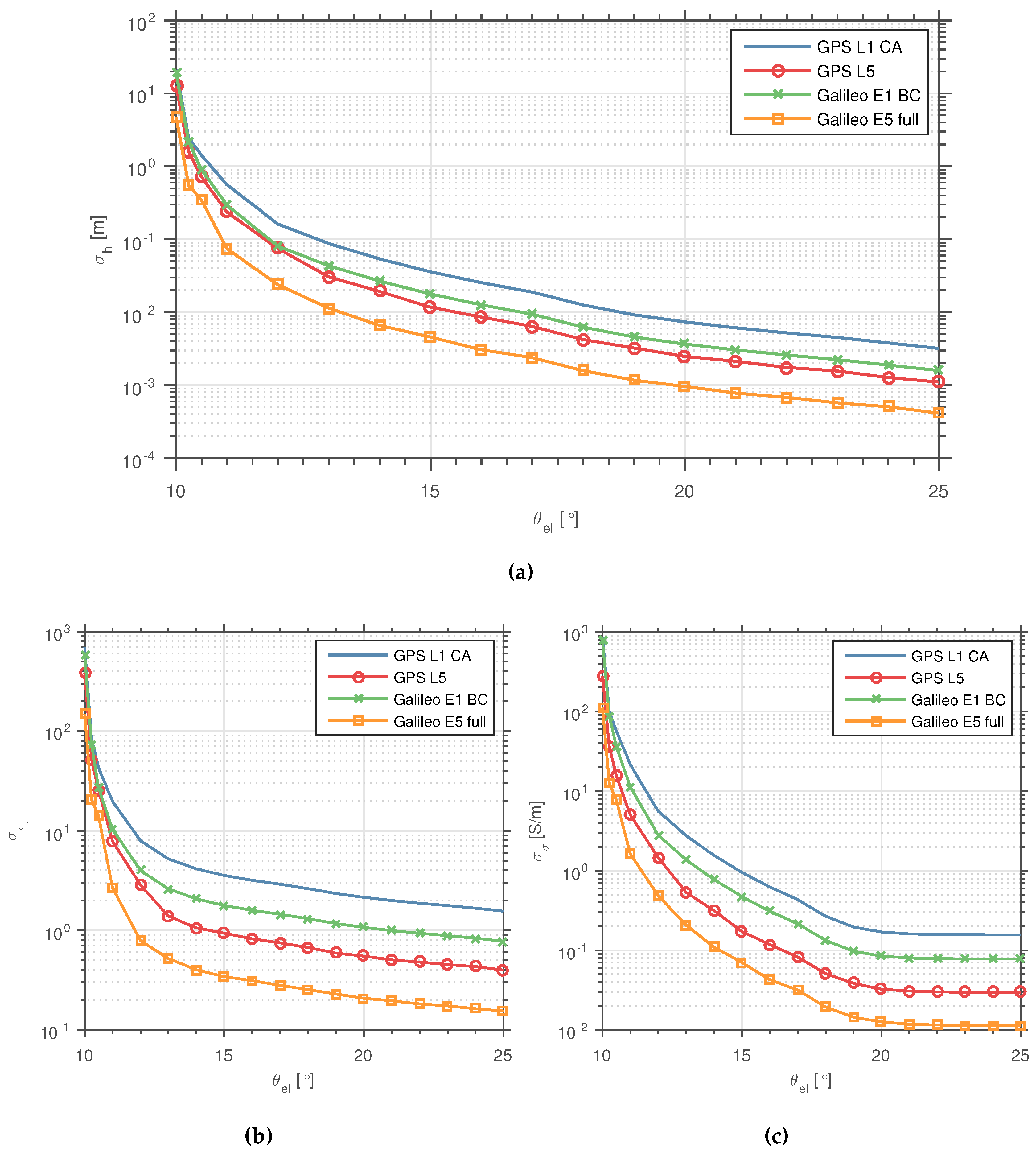
6. Analysis of the CRB()
- The propagation path difference will change due to the displacement of the specular reflection point. In addition, the angle of arrival of both the LOS and the reflected component to the antenna will also vary.
- If the reflection coefficient Γ is assumed to depend on , this will also change during the observation time.
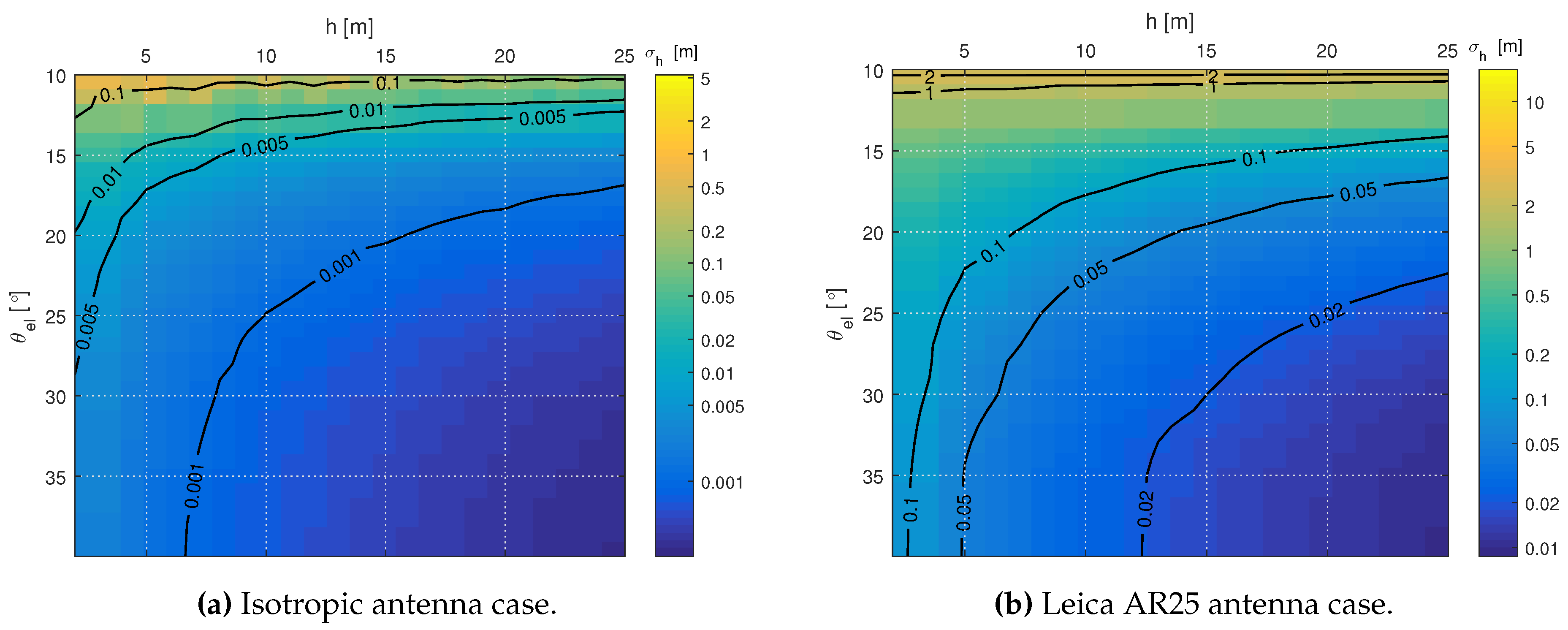
- An ideal case with an isotropic antenna model.
- A Leica GNSS AR25 antenna [74] model. Only the antenna gain’s amplitude has been modeled. The antenna phase center is assumed to be located at the distance h perpendicular to the reflection surface. The antenna boresight is pointing upwards, parallel to the surface normal vector (i.e., an elevation of 90°). We have used the pattern model provided as part of the open source GPS multipath simulator [75].
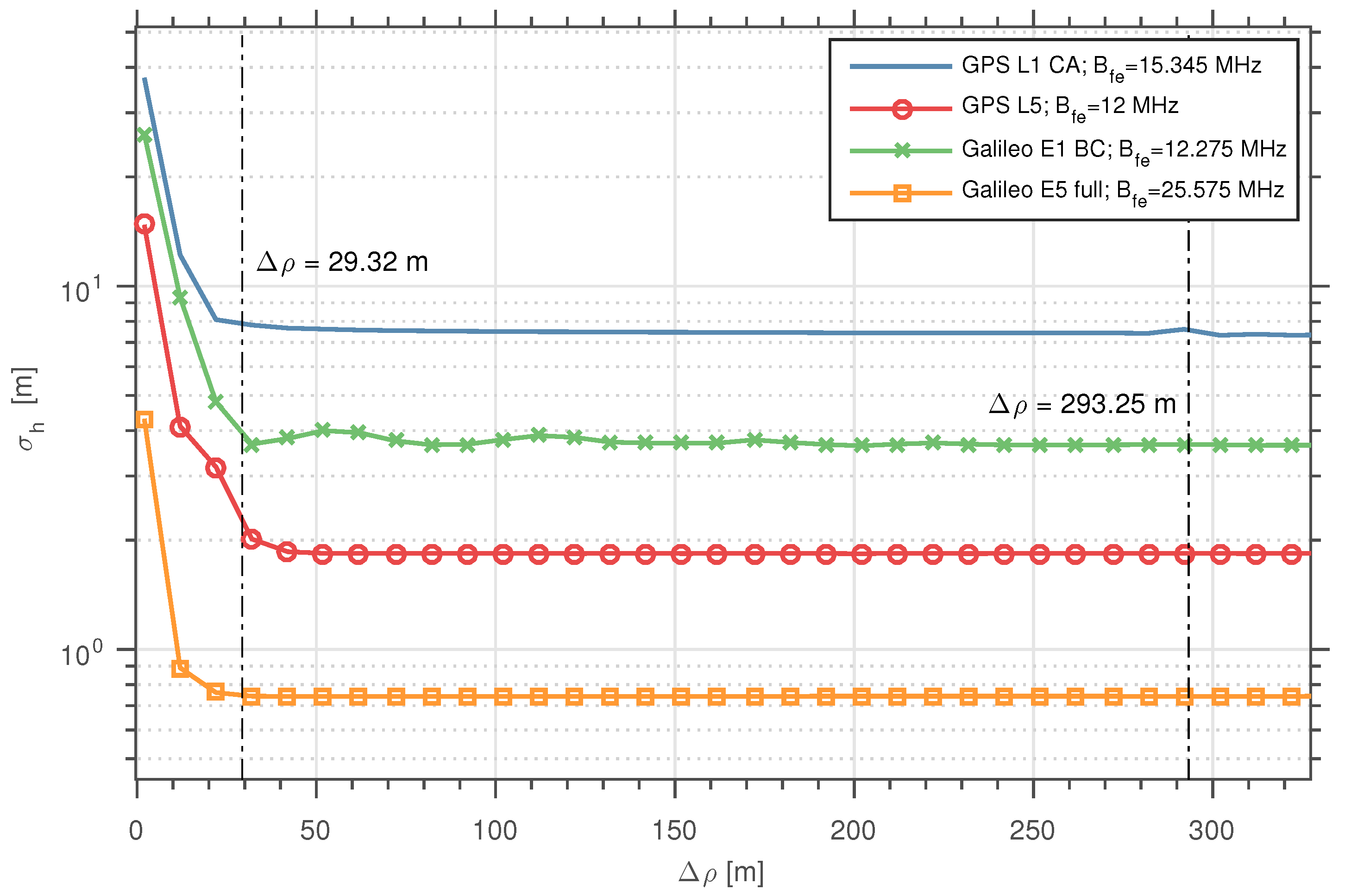
6.1. CRB() vs.
6.2. Effects of the Signal Modulation on the CRB()
7. Conclusions and Future Work
Acknowledgments
Author Contributions
Conflicts of Interest
Appendix A. Expressions for the Transformation Matrices Used and Analytic Expressions for the CRB in Short Observation Times
Appendix B. Zavorotny–Larson Model for the Surface Reflection Coefficient Γ
References
- Zavorotny, V.U.; Gleason, S.; Cardellach, E.; Camps, A. Tutorial on Remote Sensing Using GNSS Bistatic Radar of Opportunity. IEEE Geosci. Remote Sens. Mag. 2014, 2, 8–45. [Google Scholar] [CrossRef]
- Martin-Neira, M. A passive reflectometry and interferometry system (PARIS): Application to ocean altimetry. ESA J. 1993, 17, 331–355. [Google Scholar]
- Martin-Neira, M.; D’Addio, S.; Buck, C.; Floury, N.; Prieto-Cerdeira, R. The PARIS Ocean Altimeter In-Orbit Demonstrator. IEEE Trans. Geosci. Remote Sens. 2011, 49, 2209–2237. [Google Scholar] [CrossRef]
- Nogués-Correig, O.; Cardellach, E.; Campderrós, J.S.; Rius, A. A GPS-reflections receiver that computes doppler/delay maps in real time. IEEE Trans. Geosci. Remote Sens. 2007, 45, 156–174. [Google Scholar] [CrossRef]
- Camps, A.; Marchan-Hernandez, J.F.; Bosch-Lluis, X.; Rodriguez-Alvarez, N.; Ramos-Perez, I.; Valencia, E.; Tarongi, J.M.; Park, H.; Carreno-Luengo, H.; Alonso-Arroyo, A.; et al. Review of GNSS-R instruments and tools developed at the Universitat Politecnica de Catalunya-Barcelona tech. In Proceedings of the 2014 IEEE International Geoscience and Remote Sensing Symposium (IGARSS), Quebec, QC, Canada, 13–18 July 2014; pp. 3826–3829.
- Gleason, S.; Hodgart, S.; Gommenginger, C.; Mackin, S.; Adjrad, M.; Unwin, M. Detection and Processing of bistatically reflected GPS signals from low Earth orbit for the purpose of ocean remote sensing. IEEE Trans. Geosci. Remote Sens. 2005, 43, 1229–1241. [Google Scholar] [CrossRef]
- Zavorotny, V.U.; Larson, K.M.; Braun, J.J.; Small, E.E.; Gutmann, E.D.; Bilich, A.L. A Physical Model for GPS Multipath Caused by Land Reflections: Toward Bare Soil Moisture Retrievals. IEEE J-STARS 2010, 3, 100–110. [Google Scholar] [CrossRef]
- Zavorotny, V.; Voronovich, A. Scattering of GPS signals from the ocean with wind remote sensing application. IEEE Trans. Geosci. Remote Sens. 2000, 38, 951–964. [Google Scholar] [CrossRef]
- Martin, F.; DAddio, S.; Camps, A.; Martin-Neira, M. Modeling and Analysis of GNSS-R Waveforms Sample-to-Sample Correlation. IEEE J-STARS 2014, 7, 1545–1559. [Google Scholar] [CrossRef]
- Clarizia, M.P.; Gommenginger, C.P.; Gleason, S.T.; Srokosz, M.A.; Galdi, C.; Di Bisceglie, M. Analysis of GNSS-R delay-Doppler maps from the UK-DMC satellite over the ocean. Geophys. Res. Lett. 2009, 36. [Google Scholar] [CrossRef]
- Pierdicca, N.; Pulvirenti, L.; Ticconi, F.; Brogioni, M. Radar Bistatic Configurations for Soil Moisture Retrieval: A Simulation Study. IEEE Trans. Geosci. Remote Sens. 2008, 46, 3252–3264. [Google Scholar] [CrossRef]
- Pierdicca, N.; Guerriero, L.; Giusto, R.; Brogioni, M.; Egido, A. SAVERS: A Simulator of GNSS Reflections From Bare and Vegetated Soils. IEEE Trans. Geosci. Remote Sens. 2014, 52, 6542–6554. [Google Scholar] [CrossRef]
- Schiavulli, D.; Ghavidel, A.; Camps, A.; Migliaccio, M. A simulator for GNSS-R polarimetric observations over the ocean. In Proceedings of the 2014 IEEE International Geoscience and Remote Sensing Symposium (IGARSS 2014), Quebec, QC, USA, 13–18 July 2014; pp. 3802–3805.
- Jin, S.; Komjathy, A. GNSS reflectometry and remote sensing: New objectives and results. Adv. Space Res. 2010, 46, 111–117. [Google Scholar] [CrossRef]
- Cardellach, E.; Fabra, F.; Nogués-Correig, O.; Oliveras, S.; Ribó, S.; Rius, A. GNSS-R ground-based and airborne campaigns for ocean, land, ice, and snow techniques: Application to the GOLD-RTR data sets. Radio Sci. 2011, 46. [Google Scholar] [CrossRef]
- Ruf, C.; Unwin, M.; Dickinson, J.; Rose, R.; Rose, D.; Vincent, M.; Lyons, A. CYGNSS: Enabling the Future of Hurricane Prediction [Remote Sensing Satellites]. IEEE Geosci. Remote Sens. Mag. 2013, 1, 52–67. [Google Scholar] [CrossRef]
- Camps, A.; Park, H.; Ghavidel, A.; Rius, J.M.; Sekulic, I. GEROS-ISS, a demonstration mission of GNSS remote sensing capabilities to derive geophysical parameters of the earth surfaces: Altimetry performance evaluation. In Proceedings of the 2015 IEEE International Geoscience and Remote Sensing Symposium (IGARSS 2015), Milan, Italy, 26–31 July 2015; pp. 3917–3920.
- Katzberg, S.J.; Torres, O.; Grant, M.S.; Masters, D. Utilizing calibrated GPS reflected signals to estimate soil reflectivity and dielectric constant: Results from SMEX02. Remote Sens. Environ. 2006, 100, 17–28. [Google Scholar] [CrossRef]
- Larson, K.M.; Small, E.E.; Gutmann, E.D.; Bilich, A.L.; Braun, J.J.; Zavorotny, V.U. Use of GPS receivers as a soil moisture network for water cycle studies. Geophys. Res. Lett. 2008, 35, L24405. [Google Scholar] [CrossRef]
- Larson, K.M.; Braun, J.J.; Small, E.E.; Zavorotny, V.U.; Gutmann, E.D.; Bilich, A.L. GPS Multipath and Its Relation to Near-Surface Soil Moisture Content. IEEE J-STARS 2010, 3, 91–99. [Google Scholar] [CrossRef]
- Rodriguez-Alvarez, N.; Camps, A.; Vall-llossera, M.; Bosch-Lluis, X.; Monerris, A.; Ramos-Perez, I.; Valencia, E.; Marchan-Hernandez, J.F.; Martinez-Fernandez, J.; Baroncini-Turricchia, G.; et al. Land Geophysical Parameters Retrieval Using the Interference Pattern GNSS-R Technique. IEEE Trans. Geosci. Remote Sens. 2011, 49, 71–84. [Google Scholar] [CrossRef]
- Botteron, C.; Dawes, N.; Leclère, J.; Skaloud, J.; Weijs, S.; Farine, P.A. Soil Moisture & Snow Properties Determination with GNSS in Alpine Environments: Challenges, Status, and Perspectives. Remote Sens. 2013, 5, 3516–3543. [Google Scholar]
- Alonso Arroyo, A.; Camps, A.; Aguasca, A.; Forte, G.; Monerris, A.; Rudiger, C.; Walker, J.; Park, H.; Pascual, D.; Onrubia, R. Dual-Polarization GNSS-R Interference Pattern Technique for Soil Moisture Mapping. IEEE J-STARS 2014, 7, 1533–1544. [Google Scholar] [CrossRef]
- Chew, C.; Small, E.E.; Larson, K.M. An algorithm for soil moisture estimation using GPS-interferometric reflectometry for bare and vegetated soil. GPS Solut. 2015, 20, 525–537. [Google Scholar] [CrossRef]
- Roussel, N.; Frappart, F.; Ramillien, G.; Darrozes, J.; Baup, F.; Lestarquit, L.; Ha, M.C. Detection of Soil Moisture Variations Using GPS and GLONASS SNR Data for Elevation Angles Ranging From 2 deg to 70 deg. IEEE J-STARS 2016, 9, 4781–4794. [Google Scholar]
- Larson, K.M.; Gutmann, E.D.; Zavorotny, V.U.; Braun, J.J.; Williams, M.W.; Nievinski, F.G. Can we measure snow depth with GPS receivers? Geophys. Res. Lett. 2009, 36, L17502. [Google Scholar] [CrossRef]
- Larson, K.M.; Nievinski, F.G. GPS snow sensing: Results from the EarthScope Plate Boundary Observatory. GPS Solut. 2012, 17, 41–52. [Google Scholar] [CrossRef]
- Rodriguez-Alvarez, N.; Aguasca, A.; Valencia, E.; Bosch-Lluis, X.; Camps, A.; Ramos-Perez, I.; Park, H.; Vall-llossera, M. Snow Thickness Monitoring Using GNSS Measurements. IEEE Geosci. Remote Sens. Lett. 2012, 9, 1109–1113. [Google Scholar] [CrossRef]
- Nievinski, F.G.; Larson, K.M. Inverse Modeling of GPS Multipath for Snow Depth Estimation—Part II: Application and Validation. IEEE Trans. Geosci. Remote Sens. 2014, 52, 6564–6573. [Google Scholar] [CrossRef]
- Nievinski, F.G.; Larson, K.M. Inverse Modeling of GPS Multipath for Snow Depth Estimation—Part I: Formulation and Simulations. IEEE Trans. Geosci. Remote Sens. 2014, 52, 6555–6563. [Google Scholar] [CrossRef]
- Larson, K.M.; Small, E.E. Estimation of Snow Depth Using L1 GPS Signal-to-Noise Ratio Data. IEEE J-STARS 2016, 9, 4802–4808. [Google Scholar] [CrossRef]
- Vey, S.; Guntner, A.; Wickert, J.; Blume, T.; Thoss, H.; Ramatschi, M. Monitoring Snow Depth by GNSS Reflectometry in Built-up Areas: A Case Study for Wettzell, Germany. IEEE J-STARS 2016, 9, 4809–4816. [Google Scholar] [CrossRef]
- Rivas, M.; Maslanik, J.; Axelrad, P. Bistatic Scattering of GPS Signals Off Arctic Sea Ice. IEEE Trans. Geosci. Remote Sens. 2010, 48, 1548–1553. [Google Scholar] [CrossRef]
- Fabra, F.; Cardellach, E.; Rius, A.; Ribó, S.; Oliveras, S.; Nogués-Correig, O.; Belmonte Rivas, M.; Semmling, M.; D’Addio, S. Phase altimetry with dual polarization GNSS-R over sea ice. IEEE Trans. Geosci. Remote Sens. 2012, 50, 2112–2121. [Google Scholar] [CrossRef]
- Ruffini, G.; Soulat, F.; Caparrini, M.; Germain, O.; Martín-Neira, M. The Eddy experiment: Accurate GNSS-R ocean altimetry from low altitude aircraft. Geophys. Res. Lett. 2004, 31. [Google Scholar] [CrossRef]
- Bai, W.; Sun, Y.; Fu, Y.; Zhu, G.; Du, Q.; Zhang, Y.; Han, Y.; Cheng, C. GNSS-R open-loop difference phase altimetry: Results from a bridge experiment. Adv. Space Res. 2012, 50, 1150–1157. [Google Scholar] [CrossRef]
- Dampf, J.; Pany, T.; Falk, N.; Riedl, B.; Winkel, J. Galileo Altimetry Using AltBOC and RTK Techniques. Inside GNSS 2013, 8, 54–63. [Google Scholar]
- Löfgren, J.S.; Haas, R. Sea level measurements using multi-frequency GPS and GLONASS observations. EURASIP J. Adv. Signal Process. 2014, 2014, 50. [Google Scholar] [CrossRef]
- Carreno-Luengo, H.; Camps, A. Empirical Results of a Surface-Level GNSS-R Experiment in a Wave Channel. Remote Sens. 2015, 7, 7471–7493. [Google Scholar] [CrossRef] [Green Version]
- Tabibi, S.; Nievinski, F.G.; Van Dam, T.; Monico, J.F.G. Assessment of modernized GPS L5 SNR for ground-based multipath reflectometry applications. Adv. Space Res. 2015, 55, 1104–1116. [Google Scholar] [CrossRef]
- Alonso-Arroyo, A.; Camps, A.; Park, H.; Pascual, D.; Onrubia, R.; Martin, F. Retrieval of Significant Wave Height and Mean Sea Surface Level Using the GNSS-R Interference Pattern Technique: Results From a Three-Month Field Campaign. IEEE Trans. Geosci. Remote Sens. 2015, 53, 3198–3209. [Google Scholar] [CrossRef] [Green Version]
- Kucwaj, J.C.; Stienne, G.; Reboul, S.; Choquel, J.B.; Benjelloun, M. Accurate Pseudorange Estimation by Means of Code and Phase Delay Integration: Application to GNSS-R Altimetry. IEEE J-STARS 2016, 9, 4854–4864. [Google Scholar] [CrossRef]
- Lestarquit, L.; Peyrezabes, M.; Darrozes, J.; Motte, E.; Roussel, N.; Wautelet, G.; Frappart, F.; Ramillien, G.; Biancale, R.; Zribi, M. Reflectometry With an Open-Source Software GNSS Receiver: Use Case With Carrier Phase Altimetry. IEEE J-STARS 2016, 9, 4843–4853. [Google Scholar] [CrossRef]
- Ferrazzoli, P.; Guerriero, L.; Pierdicca, N.; Rahmoune, R. Forest biomass monitoring with GNSS-R: Theoretical simulations. Adv. Space Res. 2011, 47, 1823–1832. [Google Scholar] [CrossRef]
- Carreno-Luengo, H.; Amèzaga, A.; Vidal, D.; Olivé, R.; Munoz, J.; Camps, A. First Polarimetric GNSS-R Measurements from a Stratospheric Flight over Boreal Forests. Remote Sens. 2015, 7, 13120–13138. [Google Scholar] [CrossRef] [Green Version]
- Zuffada, C.; Zavorotny, V. Coherence time and statistical properties of the GPS signal scattered off the ocean surface and their impact on the accuracy of remote sensing of sea surface topography and winds. In Proceedings of the 2001 IEEE International Geoscience and Remote Sensing Symposium (IGARSS 2001), Sydney, Australia, 9–13 July 2001; pp. 3332–3334.
- Hajj, G.A.; Zuffada, C. Theoretical description of a bistatic system for ocean altimetry using the GPS signal. Radio Sci. 2003, 38. [Google Scholar] [CrossRef]
- Fischer, R. Standard Deviation of Scatterometer Measurements from Space. IEEE Trans. Geosci. Electron. 1972, 10, 106–113. [Google Scholar] [CrossRef]
- Lowe, S.T.; LaBrecque, J.L.; Zuffada, C.; Romans, L.J.; Young, L.E.; Hajj, G.A. First spaceborne observation of an Earth-reflected GPS signal. Radio Sci. 37, 7-1–7-28. [CrossRef]
- Thomas, J.B. Signal-processing theory for the TurboRogue receiver. 1995. Available online: https://ntrs.nasa.gov/search.jsp?R=19950024160 (accessed on 1 December 2016). [Google Scholar]
- Germain, O.; Ruffini, G. A revisit to the GNSS-R code range precision. In Proceedings of the GNSS-R’06 Workshop, ESA/ESTEC, Noordwijk, The Netherlands, 14–15 June 2006.
- D’Addio, S.; Martin-Neira, M.; Martin, F.; Park, H.; Camps, A. GNSS-R altimeter performance: Analysis of Cramer-Rao lower bounds. In Proceedings of the 2012 Workshop on Reflectometry Using GNSS and Other Signals of Opportunity (GNSS+R), West Lafayette, IN, USA, 10–11 October 2012.
- Camps, A.; Park, H.; Valencia i Domenech, E.; Pascual, D.; Martin, F.; Rius, A.; Ribo, S.; Benito, J.; Andres-Beivide, A.; Saameno, P.; et al. Optimization and Performance Analysis of Interferometric GNSS-R Altimeters: Application to the PARIS IoD Mission. IEEE J-STARS 2014, 7, 1436–1451. [Google Scholar] [CrossRef]
- Pascual, D.; Camps, A.; Martin, F.; Park, H.; Arroyo, A.A.; Onrubia, R. Precision Bounds in GNSS-R Ocean Altimetry. IEEE J-STARS 2014, 7, 1416–1423. [Google Scholar] [CrossRef]
- Bilich, A.; Larson, K.M.; Axelrad, P. Modeling GPS phase multipath with SNR: Case study from the Salar de Uyuni, Bolivia. J. Geophys. Res. 2008, 113, B04401. [Google Scholar] [CrossRef]
- Qian, X.; Jin, S. Estimation of Snow Depth From GLONASS SNR and Phase-Based Multipath Reflectometry. IEEE J-STARS 2016, 9, 4817–4823. [Google Scholar] [CrossRef]
- Ribot Sanfelix, M.A.; Botteron, C.; Farine, P.A. A New Estimation Algorithm for the GNSS-R Interference Pattern Technique: The Segmented Maximum-Likelihood. In Proceedings of the 28th International Technical Meeting of The Satellite Division of the Institute of Navigation (ION GNSS+ 2015), Tampa, FL, USA, 16–17 September 2015.
- Ribot, M.A.; Kucwaj, J.C.; Botteron, C.; Reboul, S.; Stienne, G.; Leclère, J.; Choquel, J.B.; Farine, P.A.; Benjelloun, M. Normalized GNSS interference pattern technique for altimetry. Sensors 2014, 14, 10234–10257. [Google Scholar] [CrossRef] [PubMed]
- Rius, A.; Cardellach, E.; Martin-Neira, M. Altimetric Analysis of the Sea-Surface GPS-Reflected Signals. IEEE Trans. Geosci. Remote Sens. 2010, 48, 2119–2127. [Google Scholar] [CrossRef]
- Gleason, S. Fading statistics of bistatically scattered GPS signals detected from ocean and land in low earth orbit. In Proceedings of the 2007 IEEE International Geoscience and Remote Sensing Symposium (IGARSS 2007), Barcelona, Spain, 23–28 July 2007; pp. 5097–5100.
- Beckmann, P.; Spizzichino, A. The Scattering of Electromagnetic Waves from Rough Surfaces; Radar Library, Artech House: Norwood, MA, USA, 1987. [Google Scholar]
- Kaplan, E.D.; Hegarty, C.J. Understanding GPS: Principles and Applications, 2nd ed.; Artech House: Norwood, MA, USA, 2006. [Google Scholar]
- Foucras, M.; Leclère, J.; Botteron, C.; Julien, O.; Macabiau, C.; Farine, P.A.; Ekambi, B. Study on the cross-correlation of GNSS signals and typical approximations. GPS Solut. 2016. [Google Scholar] [CrossRef]
- European GNSS Service Centre. Galileo Open Service, Signal In Space Interface Control Document (OS-SIS-ICD), Issue 1.2; European GNSS Service Centre: Madrid, Spain, 2015.
- Navstar GPS Space/Segment Navigation User Segment Interface, Interface Specification (IS-GPS-200E); National Coordination Office for Space-Based Positioning, Navigation, and Timing: Washington, DC, USA, 2010.
- Navstar GPS Space Segment—User Segment L5 Interfaces, Interface Specification (IS-GPS-705); National Coordination Office for Space-Based Positioning, Navigation, and Timing: Washington, DC, USA, 2003.
- Tsui, J.B.-Y. Fundamentals of Global Positioning System Receivers: A Software Approach, 2nd ed.; John Wiley & Sons: New York, NY, USA, 2005; p. 352. [Google Scholar]
- Kay, S.M. Fundamentals of Statistical Signal Processing: Estimation Theory; Prentice-Hall PTR: Englewood Cliffs, NJ, USA, 1993. [Google Scholar]
- Pany, T. Navigation Signal Processing for GNSS Software Receivers; Artech House: Norwood, MA, USA, 2010; p. 372. [Google Scholar]
- Skournetou, D.; Sayed, A.H.; Lohan, E.S. Performance of Deconvolution Methods in Estimating CBOC-Modulated Signals. Int. J. Navig. Obs. 2011, 2011, 356975. [Google Scholar] [CrossRef]
- Scharf, L.L.; Demeure, C. Statistical Signal Processing: Detection, Estimation, and Time Series Analysis; Addison-Wesley Series in Electrical and Computer Engineering; Addison-Wesley Publishing Company: Boston, MS, USA, 1991. [Google Scholar]
- Betz, J.; Kolodziejski, K. Generalized Theory of Code Tracking with an Early-Late Discriminator Part I: Lower Bound and Coherent Processing. IEEE Trans. Aerosp. Electron. Syst. 2009, 45, 1538–1556. [Google Scholar] [CrossRef]
- Betz, J.W.; Kolodziejski, K.R. Extended Theory of Early-Late Code Tracking for a Bandlimited GPS Receiver. Navigation 2000, 47, 211–226. [Google Scholar] [CrossRef]
- Leica Geosystems AG. Leica AR25—White Paper; Leica Geosystems AG: Heerbrugg, Switzerland, 2009. [Google Scholar]
- Nievinski, F.G.; Larson, K.M. An open source GPS multipath simulator in Matlab/Octave. GPS Solut. 2014, 18, 473–481. [Google Scholar] [CrossRef]
- ITU-R. Electrical Characteristics of the Surface of the Earh. Recommendation P.527-3 (03/92); ITU: Geneva, Switzerland, 1992. [Google Scholar]
- Helm, A.; Beyerle, G.; Nitschke, M. Detection of coherent reflections with GPS bipath interferometry. Available online: https://arxiv.org/abs/physics/0407091 (accessed on 3 December 2016).
- Löfgren, J.S.; Haas, R.; Scherneck, H.G. Sea level time series and ocean tide analysis from multipath signals at five GPS sites in different parts of the world. J. Geodyn. 2014, 80, 66–80. [Google Scholar] [CrossRef]
- Helm, A. GPS Altimetry with the L1 OpenGPS Receiver Using Carrier Phase-Delay Observations of Reflected GPS Signals; Scientific Technical Report STR08/10; Deutsches GeoForschungsZentrum GFZ: Potsdam, Germany, 2008. [Google Scholar] [CrossRef]
- Larson, K.M.; Löfgren, J.S.; Haas, R. Coastal sea level measurements using a single geodetic GPS receiver. Adv. Space Res. 2013, 51, 1301–1310. [Google Scholar] [CrossRef]
- Wang, J.R.; Schmugge, T.J. An Empirical Model for the Complex Dielectric Permittivity of Soils as a Function of Water Content. IEEE Trans. Geosci. Remote Sens. 1980, GE-18, 288–295. [Google Scholar] [CrossRef]
- Nievinski, F.G.; Larson, K.M. Forward modeling of GPS multipath for near-surface reflectometry and positioning applications. GPS Solut. 2014, 18, 309–322. [Google Scholar] [CrossRef]
- Lerondel, G.; Romestain, R. Fresnel coefficients of a rough interface. Appl. Phys. Lett. 1999, 74, 2740. [Google Scholar] [CrossRef]
- Rodriguez-Alvarez, N.; Bosch-Lluis, X.; Camps, A.; Vall-llossera, M.; Valencia, E.; Marchan-Hernandez, J.; Ramos-Perez, I. Soil Moisture Retrieval Using GNSS-R Techniques: Experimental Results Over a Bare Soil Field. IEEE Trans. Geosci. Remote Sens. 2009, 47, 3616–3624. [Google Scholar] [CrossRef]
- Alonso-Arroyo, A.; Camps, A.; Aguasca, A.; Forte, G.; Monerris, A.; Rudiger, C.; Walker, J.; Park, H.; Pascual, D.; Onrubia, R. Improving the Accuracy of Soil Moisture Retrievals Using the Phase Difference of the Dual-Polarization GNSS-R Interference Patterns. IEEE Geosci. Remote Sens. Lett. 2014, 11, 2090–2094. [Google Scholar] [CrossRef] [Green Version]


| Signal | (MHz) | Modulation | (MHz) | Main Lobe BW(MHz) | (MHz) |
|---|---|---|---|---|---|
| GPS L1 C/A | 1575.42 | BPSK (1) | 1.023 | 2.046 | 30.69 |
| GPS L5 | 1176.45 | BPSK (10) | 10.23 | 20.46 | 24 |
| Galileo E1 OS | 1575.42 | CBOC (6,1,1/11) | 1.023 | 14.322 | 24.55 |
| Galileo E5 full | 1191.795 | AltBOC (15,10) | 10.23 | 51.15 | 51.15 |
© 2016 by the authors; licensee MDPI, Basel, Switzerland. This article is an open access article distributed under the terms and conditions of the Creative Commons Attribution (CC-BY) license (http://creativecommons.org/licenses/by/4.0/).
Share and Cite
Ribot, M.A.; Botteron, C.; Farine, P.-A. Derivation of the Cramér-Rao Bound in the GNSS-Reflectometry Context for Static, Ground-Based Receivers in Scenarios with Coherent Reflection. Sensors 2016, 16, 2063. https://doi.org/10.3390/s16122063
Ribot MA, Botteron C, Farine P-A. Derivation of the Cramér-Rao Bound in the GNSS-Reflectometry Context for Static, Ground-Based Receivers in Scenarios with Coherent Reflection. Sensors. 2016; 16(12):2063. https://doi.org/10.3390/s16122063
Chicago/Turabian StyleRibot, Miguel Angel, Cyril Botteron, and Pierre-André Farine. 2016. "Derivation of the Cramér-Rao Bound in the GNSS-Reflectometry Context for Static, Ground-Based Receivers in Scenarios with Coherent Reflection" Sensors 16, no. 12: 2063. https://doi.org/10.3390/s16122063