
Bamboo Classification Using WorldView-2 Imagery of Giant Panda Habitat in a Large Shaded Area in Wolong, Sichuan Province, China


Abstract
:1. Introduction
2. Materials and Methods
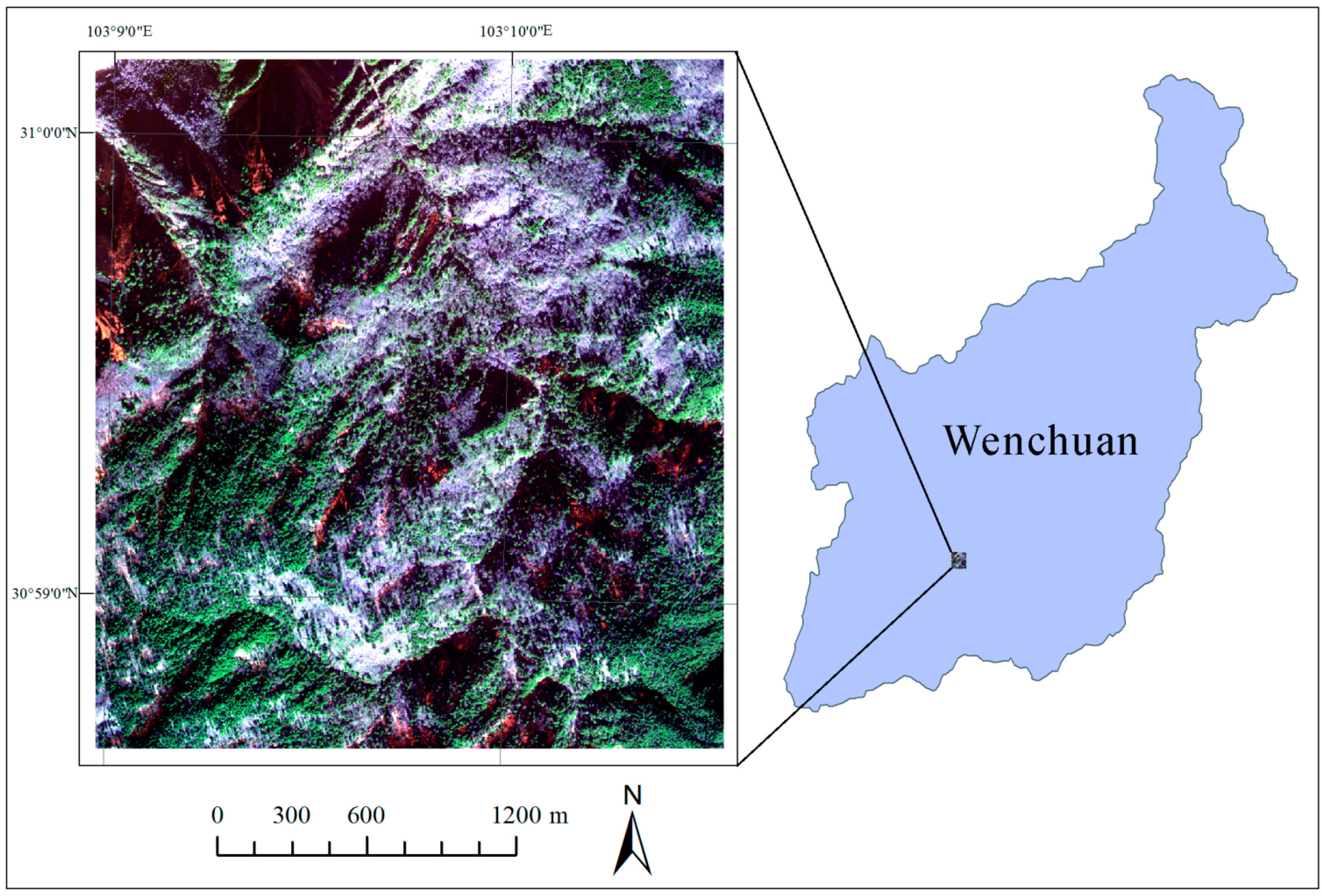
2.1. Study Area
2.2. Fieldwork
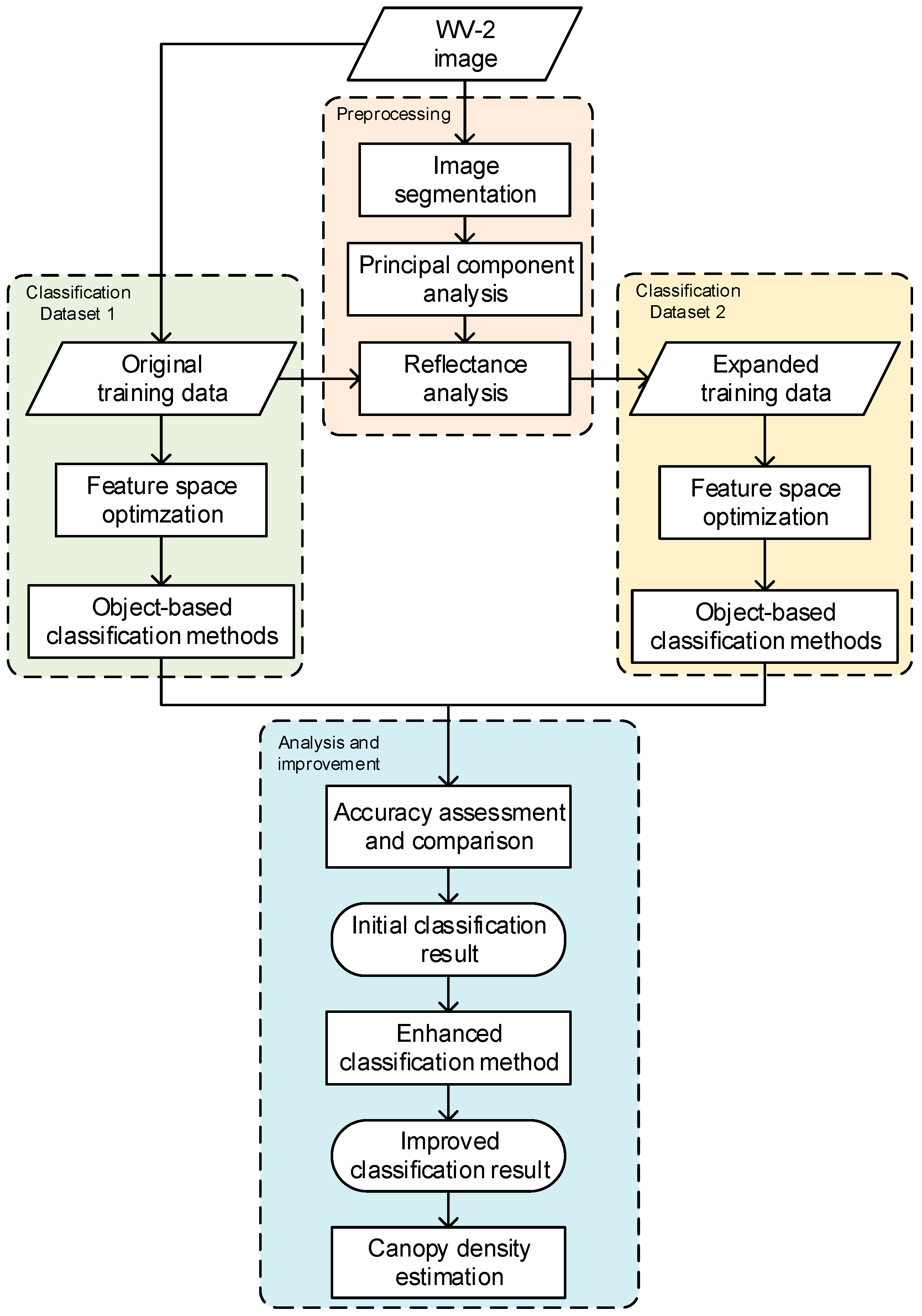
2.3. Classification Methods
3. Data Processing
3.1. Principal Component Analysis
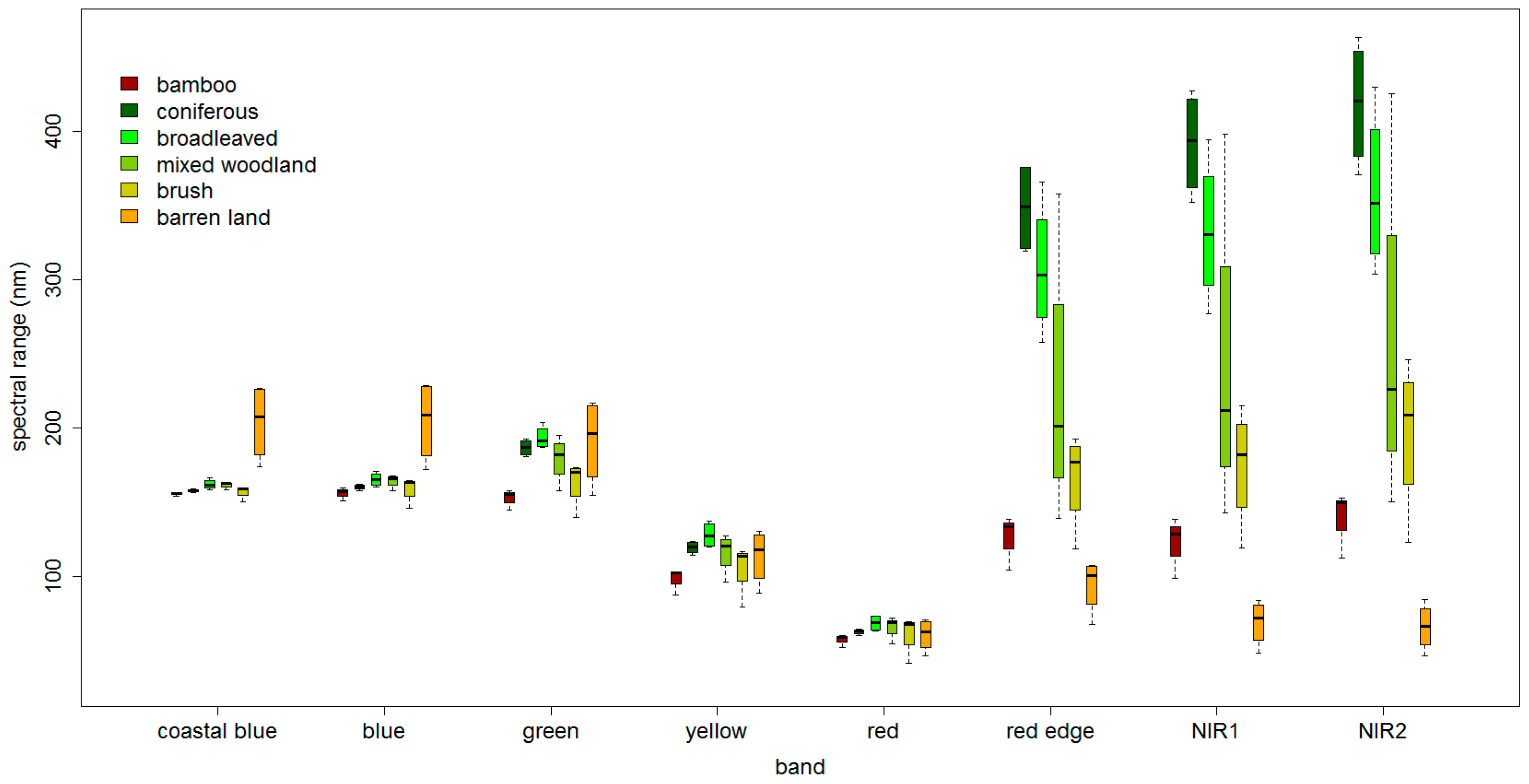
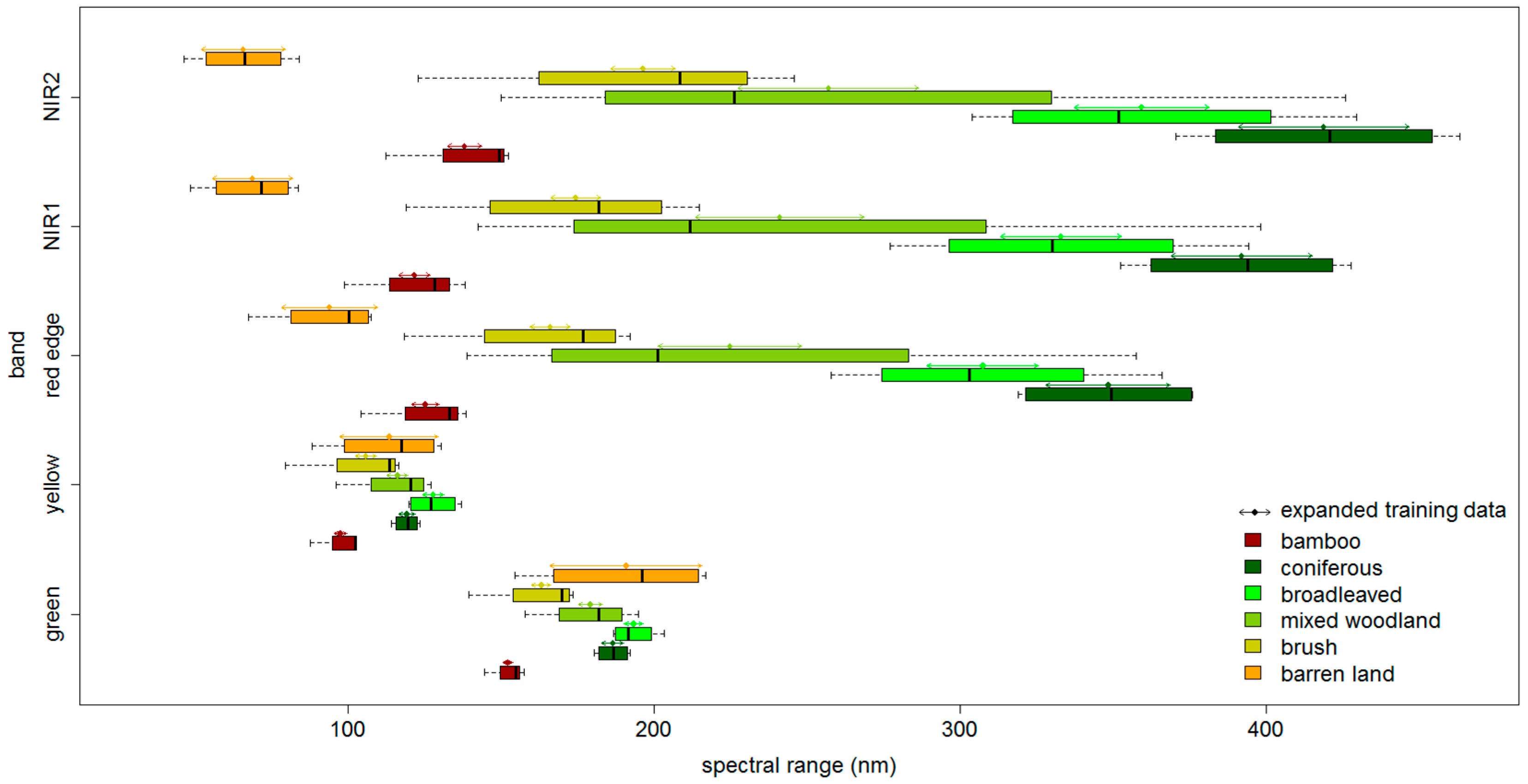
3.2. Expand Sample Size
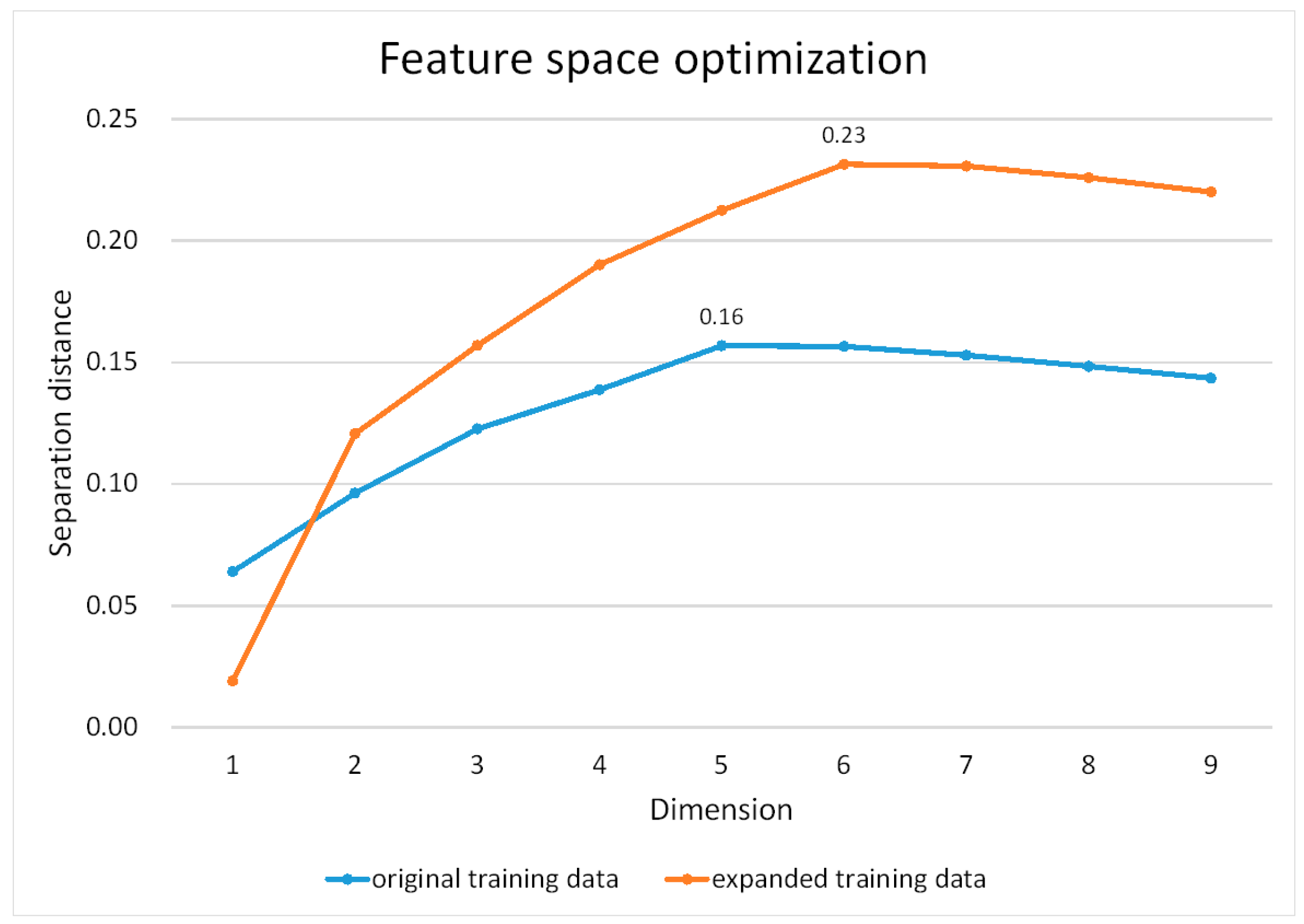
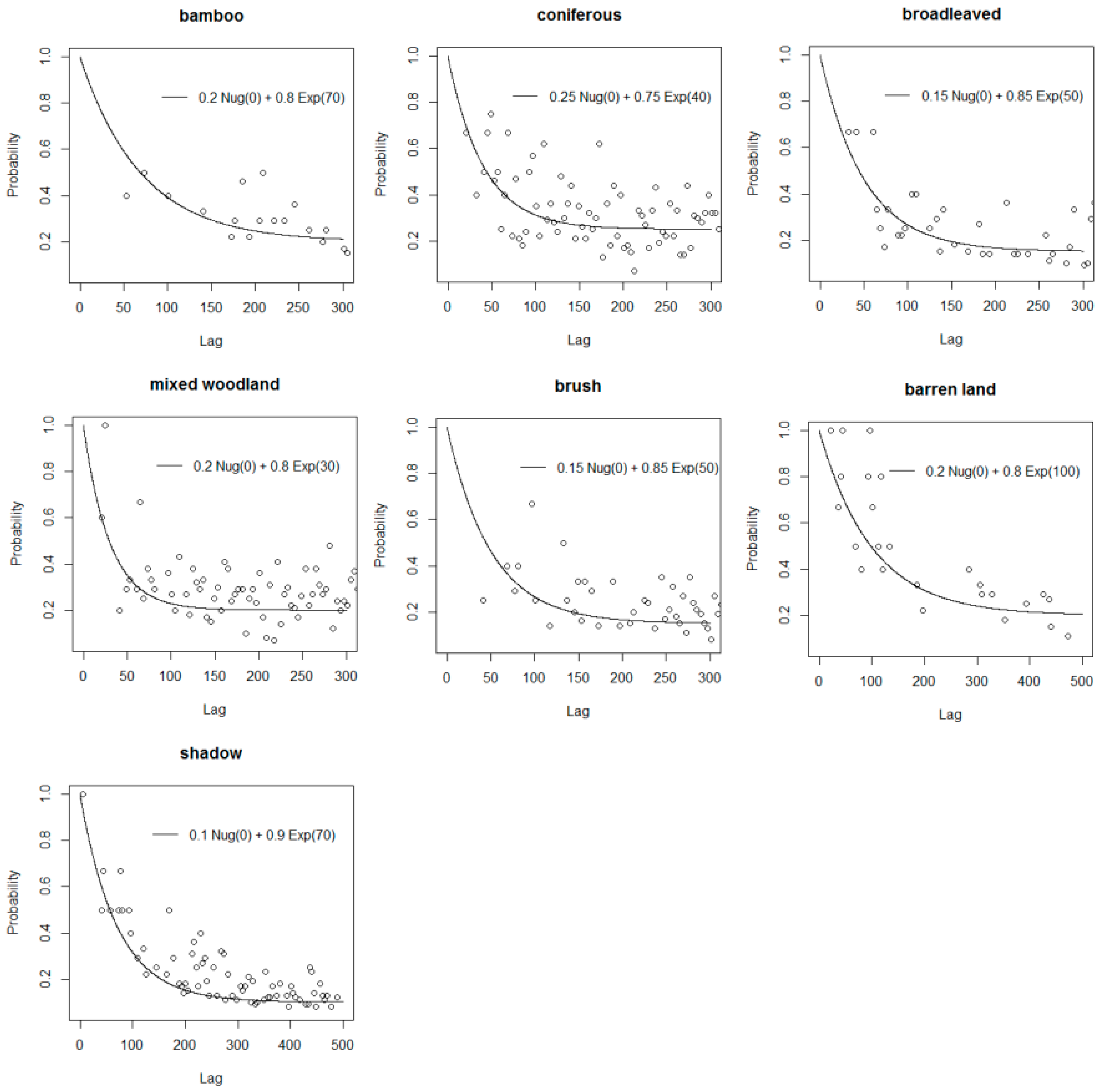
3.3. Feature Space Optimization
4. Results
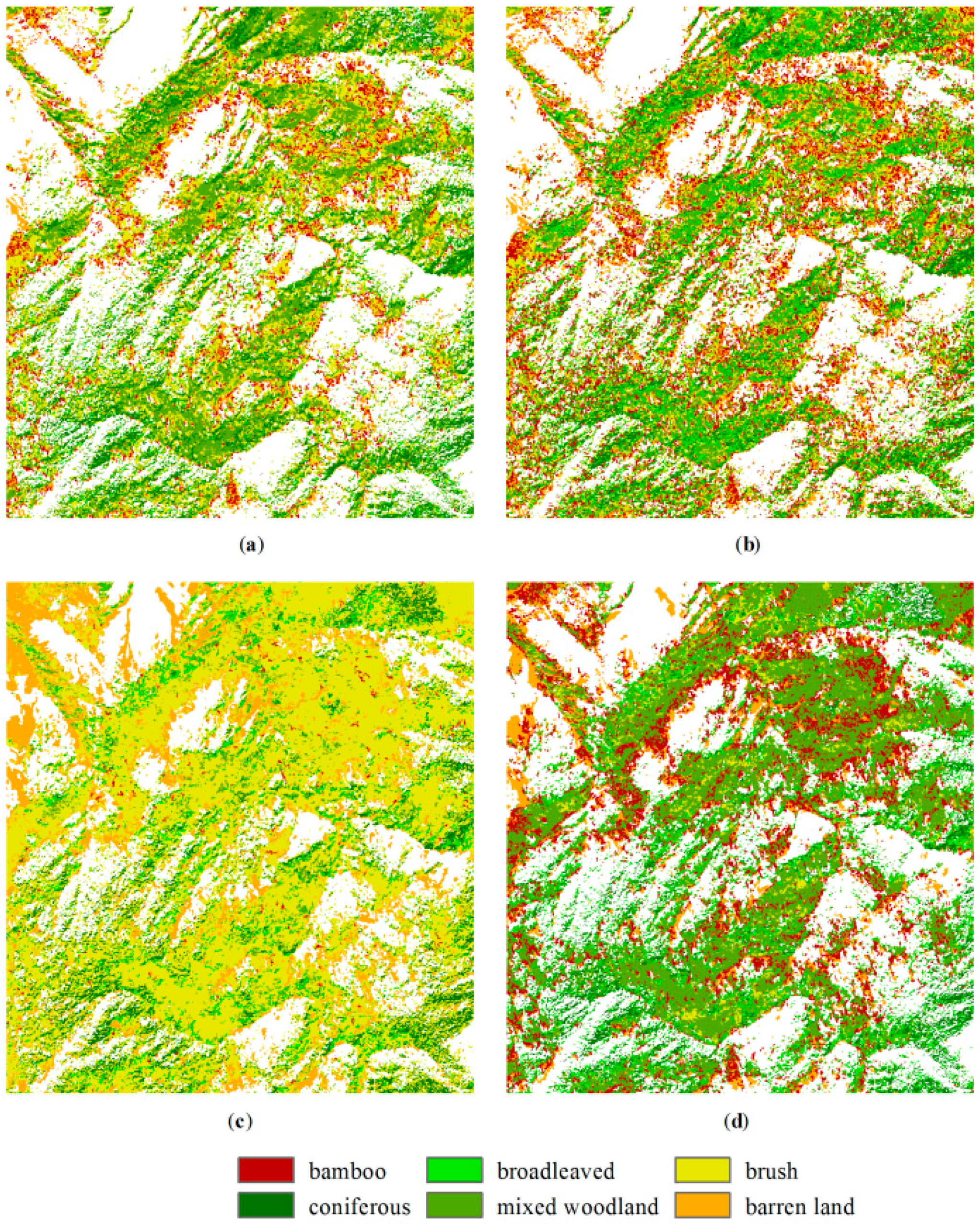
4.1. Initial Classification Results
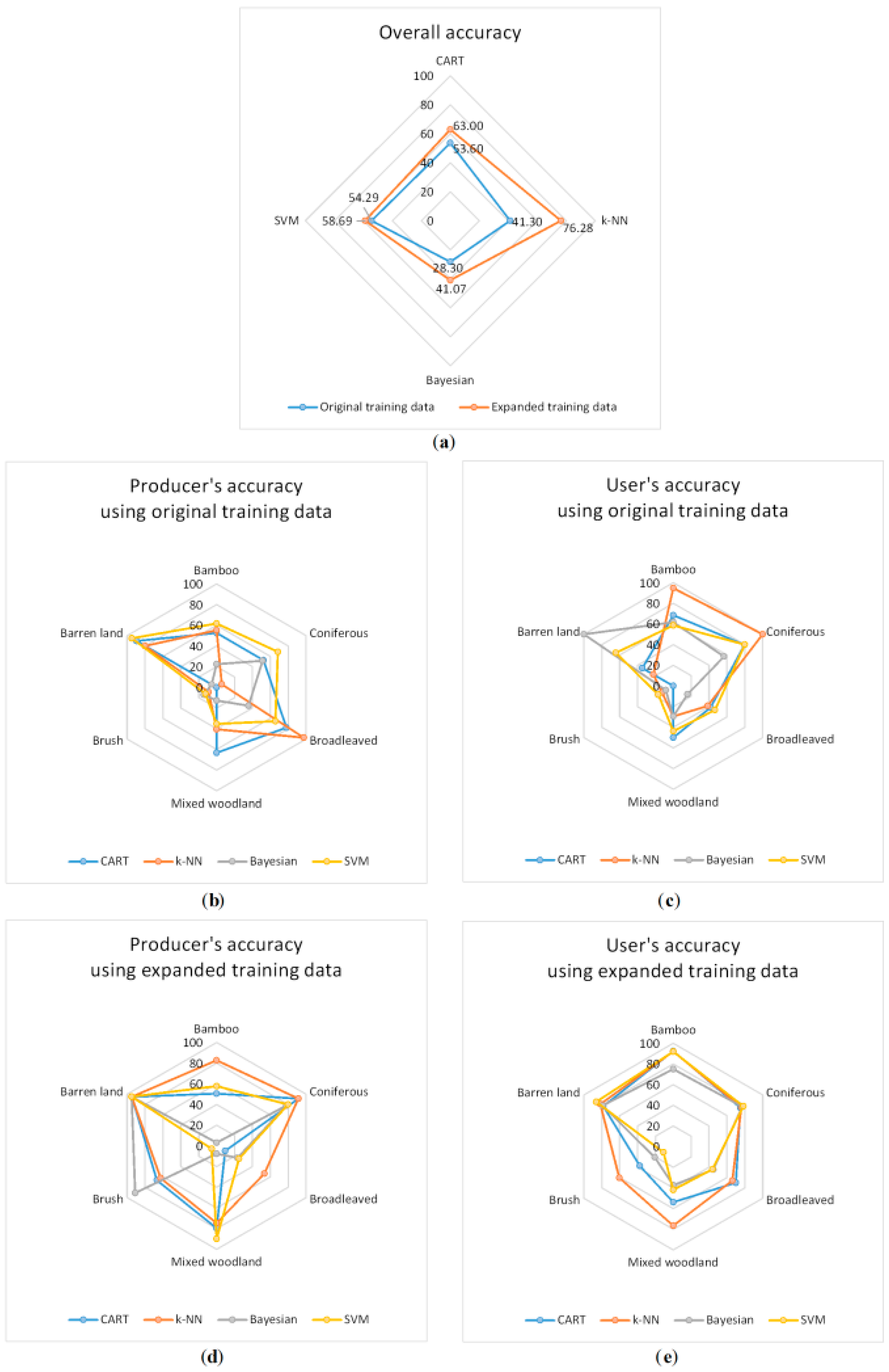
4.2. Accuracy Assessment
4.3. Improving the Classifier
5. Discussion
5.1. Canopy Density Estimation
5.2. Classification Accuracy Comparison
5.3. Performance of the Gk-NN Method
6. Conclusions
Acknowledgments
Author Contributions
Conflicts of Interest
References
- Sun, Y. Reassessing Giant Panda Habitat with Satellite-Derived Bamboo Information: A Case Study in the Qinling Mountains, China. Master’s Thesis, University of Twente, Enschede, The Netherlands, 2011. [Google Scholar]
- Viña, A.; Bearer, S.; Zhang, H.; Ouyang, Z.; Liu, J. Evaluating MODIS data for mapping wildlife habitat distribution. Remote Sens. Environ. 2008, 112, 2160–2169. [Google Scholar] [CrossRef]
- Joshi, P.K.K.; Roy, P.S.; Singh, S.; Agrawal, S.; Yadav, D. Vegetation cover mapping in India using multi-temporal IRS Wide Field Sensor (WiFS) data. Remote Sens. Environ. 2006, 103, 190–202. [Google Scholar] [CrossRef]
- Chernet, T. Comparison on the Performance of Selected Image Classification Techniques on Medium Resolution Data towards Highland Bamboo Resource Mapping. Master’s Thesis, Addis Ababa University, Addis Ababa, Ethiopia, December 2008. [Google Scholar]
- Benoit, M.; Liu, H.; Brian, B.; Manuel, R.; Fu, M.; Yang, X. Spatial patterns and processes of bamboo expansion in Southern China. Appl. Geogr. 2008, 28, 16–31. [Google Scholar]
- Wang, T.; Skidmore, A.K.; Toxopeus, A.G.; Liu, X. Understory bamboo discrimination using a winter image. Photogramm. Eng. Remote Sens. 2009, 75, 37–47. [Google Scholar] [CrossRef]
- Estes, L.D.; Reillo, P.R.; Mwangi, A.G.; Okin, G.S.; Shugart, H.H. Remote sensing of structural complexity indices for habitat and species distribution modelling. Remote Sens. Environ. 2010, 114, 792–804. [Google Scholar] [CrossRef]
- Du, H.; Cui, R.; Zhou, G.; Shi, Y.; Xu, X.; Fan, W.; Lü, Y. The responses of Moso bamboo (Phyllostachys heterocycla var. pubescens) forest aboveground biomass to Landsat TM spectral reflectance and NDVI. Acta Ecol. Sin. 2010, 30, 257–263. [Google Scholar] [CrossRef]
- Shang, Z.; Zhou, G.; Du, H.; Xu, X.; Shi, Y.; Lü, Y.; Zhou, Y.; Gu, C. Moso bamboo forest extraction and aboveground carbon storage estimation based on multi-source remotely sensed images. Int. J. Remote Sens. 2013, 34, 5351–5368. [Google Scholar] [CrossRef]
- Linderman, M.; Liu, J.; Qi, J.; An, L.; Ouyang, Z.; Yang, J.; Tan, Y. Using artificial neural networks to map the spatial distribution of understorey bamboo from remote sensing data. Int. J. Remote Sens. 2004, 25, 1685–1700. [Google Scholar] [CrossRef]
- Sesnie, S.E.; Gessler, P.E.; Finegan, B.; Thessler, S. Integrating Landsat TM and SRTM-DEM derived variables with decision trees for habitat classification and change detection in complex neotropical environments. Remote Sens. Environ. 2008, 112, 2145–2159. [Google Scholar] [CrossRef]
- Xu, X.; Du, H.; Zhou, G.; Ge, H.; Shi, Y.; Zhou, Y.; Fan, W.; Fan, W. Estimation of aboveground carbon stock of Moso bamboo (Phyllostachys heterocycla var. pubescens) forest with a Landsat Thematic Mapper image. Int. J. Remote Sens. 2011, 32, 1431–1448. [Google Scholar]
- Carvalho, A.L.D.; Nelson, B.W.; Bianchini, M.C.; Plagnol, D.; Kuplich, T.M.; Daly, D.C. Bamboo-dominated forests of the southwest Amazon: Detection, spatial extent, life cycle length and flowering waves. PLoS ONE 2013, 8. [Google Scholar] [CrossRef] [PubMed]
- Fan, J.; Li, J.; Xia, R.; Hu, L.; Wu, X.; Li, G. Assessing the impact of climate change on the habitat distribution of the giant panda in the Qinling Mountains of China. Ecol. Model. 2014, 274, 12–20. [Google Scholar] [CrossRef]
- Vyas, D.; Krishnayya, N.S.R.; Manjunath, K.R.; Ray, S.S.; Panigrahy, S. Evaluation of classifiers for processing Hyperion (EO-1) data of tropical vegetation. Int. J. Appl. Earth Obs. Geoinform. 2011, 13, 228–235. [Google Scholar] [CrossRef]
- Ghosh, A.; Joshi, P.K. A comparison of selected classification algorithms for mapping bamboo patches in lower Gangetic plains using very high resolution WorldView 2 imagery. Int. J. Appl. Earth Obs. Geoinform. 2014, 26, 298–311. [Google Scholar] [CrossRef]
- Kamagata, N.; Akamatsu, Y.; Mori, M.; Li, Q.Y.; Hoshino, Y.; Hara, K. Comparison of pixel-based and object-based classifications of high resolution satellite data in urban fringe areas. In Proceedings of the 26th Asian Conference on Remote Sensing, Hanoi, Vietnam, 7–11 November 2005.
- Ouma, Y.O.; Tateishi, R. Optimization of second-order grey-level texture in high-resolution imagery for statistical estimation of above-ground biomass. J. Environ. Inform. 2006, 8, 70–85. [Google Scholar] [CrossRef]
- Pouteau, R.; Meyer, J.-Y.; Taputuarai, R.; Stoll, B. Support vector machines to map rare and endangered native plants in Pacific islands forests. Ecol. Inform. 2012, 9, 37–46. [Google Scholar] [CrossRef]
- Sasaki, T.; Imanishi, J.; Ioki, K.; Morimoto, Y.; Kitada, K. Object-based classification of land cover and tree species by integrating airborne LiDAR and high spatial resolution imagery data. Landsc. Ecol. Eng. 2012, 8, 157–171. [Google Scholar] [CrossRef]
- Hu, Q.; Wu, W.; Xia, T.; Yu, Q.; Yang, P.; Li, Z.; Song, Q. Exploring the use of Google Earth imagery and object-based methods in land use/cover mapping. Remote Sens. 2013, 5, 6026–6042. [Google Scholar] [CrossRef]
- Araujo, L.S.; Sparovek, G.; dos Santos, J.R.; Rodrigues, R.R. High-resolution image to mapping bamboo-dominated gaps in the Atlantic rain forest, Brazil. Int. Arch. Photogramm. Remote Sens. Spat. Inform. Sci. 2008, 37, 1287–1292. [Google Scholar]
- Han, N.; Du, H.; Zhou, G.; Sun, X.; Ge, H.; Xu, X. Object-based classification using SPOT-5 imagery for Moso bamboo forest mapping. Int. J. Remote Sens. 2014, 35, 1126–1142. [Google Scholar] [CrossRef]
- DigitalGlobe. White Paper: The Benefits of the 8 Spectral Bands of WorldView-2; DigitalGlobe: Longmont, CO, USA, 2009. [Google Scholar]
- Immitzer, M.; Atzberger, C.; Koukal, T. Tree species classification with random forest using very high spatial resolution 8-band worldview-2 satellite data. Remote Sens. 2012, 4, 2661–2693. [Google Scholar] [CrossRef]
- Pu, R.; Landry, S. A comparative analysis of high spatial resolution IKONOS and WorldView-2 imagery for mapping urban tree species. Remote Sens. Environ. 2012, 124, 516–533. [Google Scholar] [CrossRef]
- Omer, G.; Mutanga, O.; Abdel-Rahman, E.M.; Adam, E. Empirical prediction of Leaf Area Index (LAI) of endangered tree species in intact and fragmented indigenous forests ecosystems using WorldView-2 data and two robust machine learning algorithms. Remote Sens. 2016, 8, 324. [Google Scholar] [CrossRef]
- Kalson, M.; Reese, H.; Ostwald, M. Tree crown mapping in managed woodlands (parklands) of semi-arid West Africa using WorldView-2 imagery and geographic object based image analysis. Sensors 2014, 14, 22643–22669. [Google Scholar] [CrossRef] [PubMed]
- Chuang, Y.-C.M.; Shiu, Y.-S. A comparative analysis of machine learning with WorldView-2 pan-sharpened imagery for tea crop mapping. Sensors 2016, 16, 594. [Google Scholar] [CrossRef] [PubMed]
- Jensen, J.R.; Cowen, D.C. Remote sensing of urban suburban infrastructure and socio-economic attributes. Photogramm. Eng. Remote Sens. 1999, 65, 611–622. [Google Scholar]
- Ehlers, M.; Gahler, M.; Janowsky, R. Automated analysis of ultra high resolution remote sensing data for biotope type mapping: New possibilities and challenges. ISPRS J. Photogramm. Remote Sens. 2003, 57, 315–326. [Google Scholar] [CrossRef]
- Yu, Q.; Gong, P.; Clinton, N.; Biging, G.; Kelly, M.; Schirokauer, D. Object-based detailed vegetation classification with airborne high spatial resolution remote sensing imagery. Photogramm. Eng. Remote Sens. 2006, 72, 799–811. [Google Scholar] [CrossRef]
- Wang, G.; Liu, J.; He, G. A method of spatial mapping and reclassification for high-spatial-resolution remote sensing image classification. Sci. World J. 2013, 2013, 1–7. [Google Scholar] [CrossRef] [PubMed]
- Blaschke, T.; Strobl, J. What’s wrong with pixels? Some recent developments interfacing remote sensing and GIS. GIS Z. Geoinform. Syst. 2001, 14, 12–17. [Google Scholar]
- Blaschke, T. Object-based contextual image classification built on image segmentation. In Proceedings of the 2003 IEEE Workshop on Advances in Techniques for Analysis of Remotely Sensed Data, Greenbelt, MD, USA, 27–28 October 2003; pp. 113–119.
- Oruc, M.; Marangoz, A.M.; Buyuksalih, G. Comparison of pixel-based and object-oriented classification approaches using Landsat-7 ETM spectral bands. In Proceedings of the ISPRS 2004 Annual Conference, Istanbul, Turkey, 19–23 July 2004.
- Araya, Y.H.; Hergarten, C. A comparison of pixel and object-based land cover classification: A case study of the Asmara region, Eritrea. Geo-Environ. Landsc. Evol. III 2008, 100, 233–243. [Google Scholar]
- Myint, S.W.; Gober, P.; Brazel, A.; Grossman-Clarke, S.; Weng, Q. Per-pixel vs. object-based classification of urban land cover extraction using high spatial resolution imagery. Remote Sens. Environ. 2011, 115, 1145–1161. [Google Scholar] [CrossRef]
- Zhang, C.; Xie, Z. Combining object-based texture measures with a neural network for vegetation mapping in the Everglades from hyperspectral imagery. Remote Sens. Environ. 2012, 124, 310–320. [Google Scholar] [CrossRef]
- Laurent, V.C.E.; Verhoef, W.; Damm, A.; Schaepman, M.E.; Clevers, J.G.P.W. A Bayesian object-based approach for estimating vegetation biophysical and biochemical variables from at-sensor APEX data. Remote Sens. Environ. 2013, 139, 6–17. [Google Scholar] [CrossRef]
- Van Coillie, F.M.B.; Verbeke, L.P.C.; de Wulf, R.R. Feature selection by genetic algorithms in object-based classification of IKONOS imagery for forest mapping in Flanders, Belgium. Remote Sens. Environ. 2007, 110, 476–487. [Google Scholar] [CrossRef]
- Zhou, W.; Huang, G.; Troy, A.; Cadenasso, M.L. Object-based land cover classification of shaded areas in high spatial resolution imagery of urban areas: A comparison study. Remote Sens. Environ. 2009, 113, 1769–1777. [Google Scholar] [CrossRef]
- Gitas, I.Z.; Mitri, G.H.; Ventura, G. Object-based image classification for burned area mapping of Creus Cape, Spain, using NOAA-AVHRR imagery. Remote Sens. Environ. 2004, 92, 409–413. [Google Scholar] [CrossRef]
- Franklin, S.E.; Hall, R.J.; Moskal, L.M.; Maudie, A.J.; Lavigne, M.B. Incorporating texture into classification of forest species composition from airborne multispectral images. Int. J. Remote Sens. 2000, 21, 61–79. [Google Scholar] [CrossRef]
- Arcidiacono, C.; Porto, S.M.C. Pixel-based classification of high-resolution satellite images for crop-shelter coverage recognition. Acta Hortic. 2012, 937, 1003–1010. [Google Scholar] [CrossRef]
- Arcidiacono, C.; Porto, S.M.C.; Casone, G. Accuracy of crop-shelter thematic maps: A case study of maps obtained by spectral and textural classification of high-resolution satellite images. J. Food Agric. Environ. 2012, 10, 1071–1074. [Google Scholar]
- Arcidiacono, C.; Porto, S.M.C. Improving per-pixel classification of crop-shelter coverage by texture analyses of high-resolution satellite panchromatic images. J. Agric. Eng. 2011, 4, 9–16. [Google Scholar]
- Agüera, F.; Aguilar, F.J.; Aguilar, M.A. Using texture analysis to improve per-pixel classification of very high resolution images for mapping plastic greenhouses. ISPRS J. Photogramm. Remote Sens. 2008, 63, 635–646. [Google Scholar] [CrossRef]
- Tobler, W.R. A computer movie simulating urban growth in the Detroit region. Econ. Geogr. 1970, 46, 234–240. [Google Scholar] [CrossRef]
- Schaller, G.B.; Hu, J.; Pan, W.; Zhu, J. The Giant Pandas of Wolong; University of Chicago Press: Chicago, IL, USA, 1985. [Google Scholar]
- Steele, B.M.; Redmond, R.L. A method of exploiting spatial information for improving classification rules: Application to the construction of polygon-based land cover maps. Int. J. Remote Sens. 2001, 22, 3143–3166. [Google Scholar] [CrossRef]
- Atkinson, P.M.; Naser, D.K. A geostatistically weighted k-NN classifier for remotely sensed imagery. Geogr. Anal. 2010, 42, 204–225. [Google Scholar] [CrossRef]
- Tang, Y.; Jing, L.; Li, H.; Atkinson, P.M. A multiple-point spatially weighted k-NN method for object-based classification. Int. J. Appl. Earth Obs. Geoinform. 2016, 52, 263–274. [Google Scholar] [CrossRef]
- Haara, A.; Haarala, M. Tree species classification using semi-automatic delineation of trees on aerial images. Scand. J. For. Res. 2002, 17, 556–565. [Google Scholar] [CrossRef]
- Puttonen, E.; Litkey, P.; Hyyppä, J. Individual tree species classification by illuminated-shaded area separation. Remote Sens. 2009, 2, 19–35. [Google Scholar] [CrossRef]
- Waser, L.T.; Klonus, S.; Ehlers, M.; Küchler, M.; Jung, A. Potential of digital sensors for land cover and tree species classifications—A case study in the framework of the DGPF-project. Photogramm. Fernerkund. Geoinform. 2010, 2010, 141–156. [Google Scholar] [CrossRef]
- Boschetti, M.; Boschetti, L.; Oliveri, S.; Casati, L.; Canova, I. Tree species mapping with airborne hyper-spectral MIVIS data: The Ticino Park study case. Int. J. Remote Sens. 2007, 28, 1251–1261. [Google Scholar] [CrossRef]
- Voss, M.; Sugumaran, R. Seasonal effect on tree species classification in an urban environment using hyperspectral data, LiDAR, and an object-oriented approach. Sensors 2008, 8, 3020–3036. [Google Scholar] [CrossRef]
- Jones, T.G.; Coops, N.C.; Sharma, T. Assessing the utility of airborne hyperspectral and LiDAR data for species distribution mapping in the coastal Pacific Northwest, Canada. Remote Sens. Environ. 2010, 114, 2841–2852. [Google Scholar] [CrossRef]
- Dalponte, M.; Bruzzone, L.; Gianelle, D. Tree species classification in the Southern Alps based on the fusion of very high geometrical resolution multispectral/hyperspectral images and LiDAR data. Remote Sens. Environ. 2012, 123, 258–270. [Google Scholar] [CrossRef]
- Jusoff, K. Mapping bamboo in Berangkat forest reserve, Kelantan, Malaysia using airborne hyperspectral imaging sensor. Int. J. Energ. Environ. 2007, 1, 1–6. [Google Scholar]
- Jian, J.; Jiang, H.; Zhou, G.; Jiang, Z.; Yu, S.; Peng, S.; Liu, S.; Wang, J. Mapping the vegetation changes in giant panda habitat using Landsat remotely sensed data. Int. J. Remote Sens. 2011, 32, 1339–2356. [Google Scholar] [CrossRef]
- Chen, L.; Lin, H.; Wang, G.; Sun, H.; Yan, E. Spectral unmixing of MODIS data based on improved endmember purification model: Application to forest type identification. In Proceedings of the 2014 Third International Workshop on Earth Observation and Remote Sensing Applications, Changsha, China, 11–14 June 2014.
- Zhang, R.; Luo, H.; Zhou, Y.; Liu, G. Discussion on possibility of the identification of karst vegetation communities based on OLI data. In Proceedings of the 2014 Third International Conference on Agro-Geoinformatics, Beijing, China, 11–14 August 2014.
- Amaral, C.H.; Roberts, D.A.; Almeida, T.I.R.; Filho, C.R.S. Mapping invasive species and spectral mixture relationships with Neotropical woody formations in southeastern Brazil. ISPRS J. Photogramm. Remote Sens. 2015, 108, 80–93. [Google Scholar] [CrossRef]


| PC1 | PC2 | PC3 | PC4 | PC5 | PC6 | PC7 | PC8 | PC9 | PC10 | |
|---|---|---|---|---|---|---|---|---|---|---|
| Standard deviation | 188 | 50 | 22 | 15 | 10 | 6 | 4 | 2 | 2 | 1 |
| Proportion of variance | 0.91 | 0.06 | 0.01 | 0.01 | 0 | 0 | 0 | 0 | 0 | 0 |
| Cumulative proportion | 0.91 | 0.98 | 0.99 | 1 | 1 | 1 | 1 | 1 | 1 | 1 |
| PC1 | PC2 | PC3 | PC4 | PC5 | PC6 | PC7 | PC8 | PC9 | PC10 | |
|---|---|---|---|---|---|---|---|---|---|---|
| Band 1 | −0.20 | 0.47 | 0.43 | |||||||
| Band 2 | −0.35 | −0.14 | −0.24 | 0.63 | 0.39 | −0.74 | ||||
| Band 3 | −0.14 | −0.54 | −0.22 | −0.46 | −0.65 | 0.48 | ||||
| Band 4 | −0.12 | −0.53 | −0.11 | 0.11 | −0.36 | 0.67 | −0.11 | |||
| Band 5 | −0.40 | −0.14 | −0.18 | −0.44 | −0.33 | 0.59 | 0.30 | |||
| Band 6 | −0.48 | 0.32 | 0.77 | 0.14 | 0.20 | −0.35 | ||||
| Band 7 | −0.57 | 0.23 | −0.76 | −0.10 | 0.16 | |||||
| Band 8 | −0.63 | 0.17 | 0.48 | −0.55 | −0.14 | |||||
| Length/width | −0.14 | |||||||||
| Border index | ||||||||||
| Shape index | ||||||||||
| GLCM 1 | −0.45 | |||||||||
| GLCM 2 | −0.56 | |||||||||
| GLCM 3 | ||||||||||
| GLCM 4 | 0.97 | −0.15 | ||||||||
| GLCM 5 | −0.52 | |||||||||
| GLCM 6 | −0.43 | |||||||||
| GLCM 7 | ||||||||||
| GLCM 8 |
| Class | t | Spectral Range (Green, Yellow, Red Edge, NIR1, NIR2) | Sample Size |
|---|---|---|---|
| Bamboo | 0.25 | (150.6, 154.0), (95.6, 99.9), (120.7, 129.9), (116.7, 126.9), (132.6, 143.7) | 49 |
| Coniferous | 0.65 | (183.0, 190.2), (116.6, 122.1), (328.0, 368.7),(368.7, 415.1), (390.8, 446.5) | 212 |
| Broadleaved | 0.4 | (190.2, 196.4), (124.5, 131.3), (289.1, 325.5),(313.1, 352.6), (337.3, 381.2) | 103 |
| Mixed woodland | 0.25 | (175.4, 183.2), (112.8, 119.6), (201.4, 248.1),(213.7, 268.5), (227.4, 286.5) | 209 |
| Brush | 0.2 | (160.0, 166.4), (102.4, 109.5), (159.5, 172.7),(166.3, 182.6), (186.0, 206.9) | 107 |
| Barren land | 0.85 | (166.0, 215.7), (97.4, 129.7), (78.3, 109.7),(55.8, 82.1), (52.3, 79.6) | 38 |
| k-NN | 1 | 2 | 3 | 4 | 5 | 6 | User’s Accuracy |
|---|---|---|---|---|---|---|---|
| 1 | 81 | 0 | 0 | 0 | 7 | 0 | 92.05% |
| 2 | 0 | 96 | 29 | 1 | 0 | 0 | 76.19% |
| 3 | 1 | 2 | 39 | 11 | 6 | 0 | 66.10% |
| 4 | 0 | 5 | 4 | 59 | 8 | 1 | 76.62% |
| 5 | 13 | 2 | 1 | 7 | 35 | 0 | 60.34% |
| 6 | 3 | 0 | 0 | 1 | 0 | 18 | 81.82% |
| Producer’s Accuracy | 82.65% | 91.43% | 53.42% | 74.68% | 62.50% | 94.74% | 76.28% |
| gk-NN | 1 | 2 | 3 | 4 | 5 | 6 | User’s Accuracy |
|---|---|---|---|---|---|---|---|
| 1 | 81 | 0 | 0 | 0 | 6 | 0 | 93.10% |
| 2 | 0 | 95 | 10 | 1 | 0 | 0 | 89.62% |
| 3 | 0 | 3 | 56 | 7 | 5 | 0 | 78.87% |
| 4 | 0 | 5 | 3 | 62 | 8 | 0 | 79.49% |
| 5 | 14 | 2 | 4 | 8 | 37 | 1 | 56.06% |
| 6 | 3 | 0 | 0 | 1 | 0 | 18 | 81.82% |
| Producer’s Accuracy | 82.65% | 90.48% | 76.71% | 78.48% | 66.07% | 94.74% | 81.16% |
| Image | Assistant Data | Methods | Class Number | Bamboo Accuracy (%) (PA/UA) 1 | Overall Accuracy (%) | Understory Bamboo | Reference |
|---|---|---|---|---|---|---|---|
| Landsat TM | - | ANN 2 | 3 | 65/85 | 80 | Yes | [10] |
| Airborne hyperspectral image | - | SAM 3 | 1 | 60 | 60 | No | [61] |
| Landsat ETM+ | Elevation, temperature, rainfall | MLC | 5 | 84/41 | 88 | No | [4] |
| ASTER | Elevation | ANN | 7 | 77/84 | 74 | Yes | [6] |
| MODIS | Elevation | MaxEnt | 2 | Kappa 0.74 | 88 | Yes | [1] |
| Landsat MSS, TM, ETM+ | - | MLC | 12 | n.s. 4 | 74 | Yes | [62] |
| Hyperion EO-1 | - | ANN | 8 | 89/87 | 81 | No | [15] |
| Digital photograph | LiDAR | Decision tree | 16 | 57/56 | 48 | No | [20] |
| Landsat TM, MODIS | - | Matched filtering | 5 | 85 | 93 | No | [9] |
| Landsat TM, MODIS | - | Unmixing | 7 | 80/77 | 86 | No | [63] |
| Landsat 8 OLI | Elevation | BPNN 5 | 12 | 84/n.s. | 87 | No | [64] |
| SPOT-5 | - | CART | 7 | 93/90 | 85 | No | [23] |
| WV-2 | - | SVM | 7 | 94/89 | 91 | No | [16] |
| VSWIR | - | EMC 6 | 8 | 72/98 | 65 | No | [65] |
© 2016 by the authors; licensee MDPI, Basel, Switzerland. This article is an open access article distributed under the terms and conditions of the Creative Commons Attribution (CC-BY) license (http://creativecommons.org/licenses/by/4.0/).
Share and Cite
Tang, Y.; Jing, L.; Li, H.; Liu, Q.; Yan, Q.; Li, X. Bamboo Classification Using WorldView-2 Imagery of Giant Panda Habitat in a Large Shaded Area in Wolong, Sichuan Province, China. Sensors 2016, 16, 1957. https://doi.org/10.3390/s16111957
Tang Y, Jing L, Li H, Liu Q, Yan Q, Li X. Bamboo Classification Using WorldView-2 Imagery of Giant Panda Habitat in a Large Shaded Area in Wolong, Sichuan Province, China. Sensors. 2016; 16(11):1957. https://doi.org/10.3390/s16111957
Chicago/Turabian StyleTang, Yunwei, Linhai Jing, Hui Li, Qingjie Liu, Qi Yan, and Xiuxia Li. 2016. "Bamboo Classification Using WorldView-2 Imagery of Giant Panda Habitat in a Large Shaded Area in Wolong, Sichuan Province, China" Sensors 16, no. 11: 1957. https://doi.org/10.3390/s16111957
APA StyleTang, Y., Jing, L., Li, H., Liu, Q., Yan, Q., & Li, X. (2016). Bamboo Classification Using WorldView-2 Imagery of Giant Panda Habitat in a Large Shaded Area in Wolong, Sichuan Province, China. Sensors, 16(11), 1957. https://doi.org/10.3390/s16111957