
Mechanical Fault Diagnosis of High Voltage Circuit Breakers Based on Variational Mode Decomposition and Multi-Layer Classifier


Abstract
:1. Introduction
2. Vibration Data Acquisition and Fault Diagnosis Process
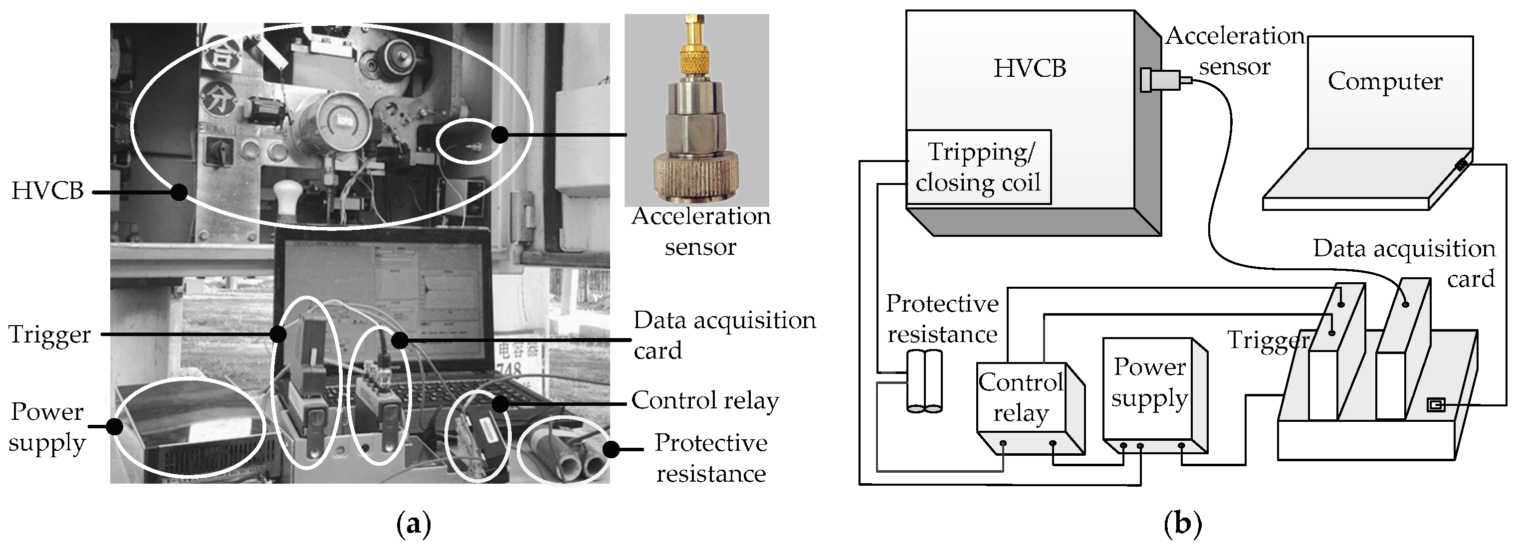
2.1. Acceleration Sensor
2.2. Data Acquisition System
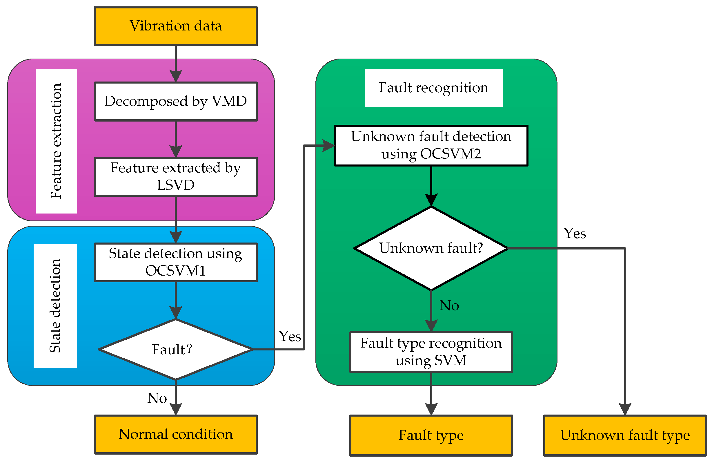
2.3. Fault Diagnosis Process
3. VMD
3.1. VMD Theory
- Construction of the variational problemThe VMD turns an input signal h into K modes. Each mode mk is mostly compact around a center frequency ωk. The variational problem can be described as seeking the K modes to make the sum of all bandwidths of the modes minimum. The constraint condition is that the sum of each mode is equals to the input signal h. The detailed construction scheme is as follows: (1) The associated analytic signal of each mode mk is computed by the Hilbert transform to obtain the unilateral frequency spectrum; (2) The frequency spectrum of each mode is tuned to the respective estimated center frequency by mixing with the exponential ; (3) The bandwidth is estimated through the squared L2-norm of the gradient of the demodulated signal. The constrained variational problem is written as:where is the set of all modes, are the corresponding center frequencies, is the Dirac function, and * denotes the convolution.
- Solution of the variational problemA constrained variational problem can become unconstrained by introducing a Lagrange multiplier α and a quadratic penalty factor η. The Lagrange multiplier enforces constraints strictly; and the quadratic penalty factor guarantees the reconstruction fidelity of the signal with Gaussian noise. The augmented Lagrange expression is as follows [29]:The alternating direction method of multipliers (ADMM) solves the saddle point of the augmented Lagrange. and are alternately updated using the ADMM approach. The updates of and are as follows (see Appendix A for the detailed solution process):where denotes the FT of , and is the update parameter of the Lagrange multiplier. The mode can be obtained as the real part of the inverse FT of . VMD estimates the mode mk and center frequency ωk constantly through an iteration. For a given convergence tolerance e > 0, the termination condition of this iteration is:
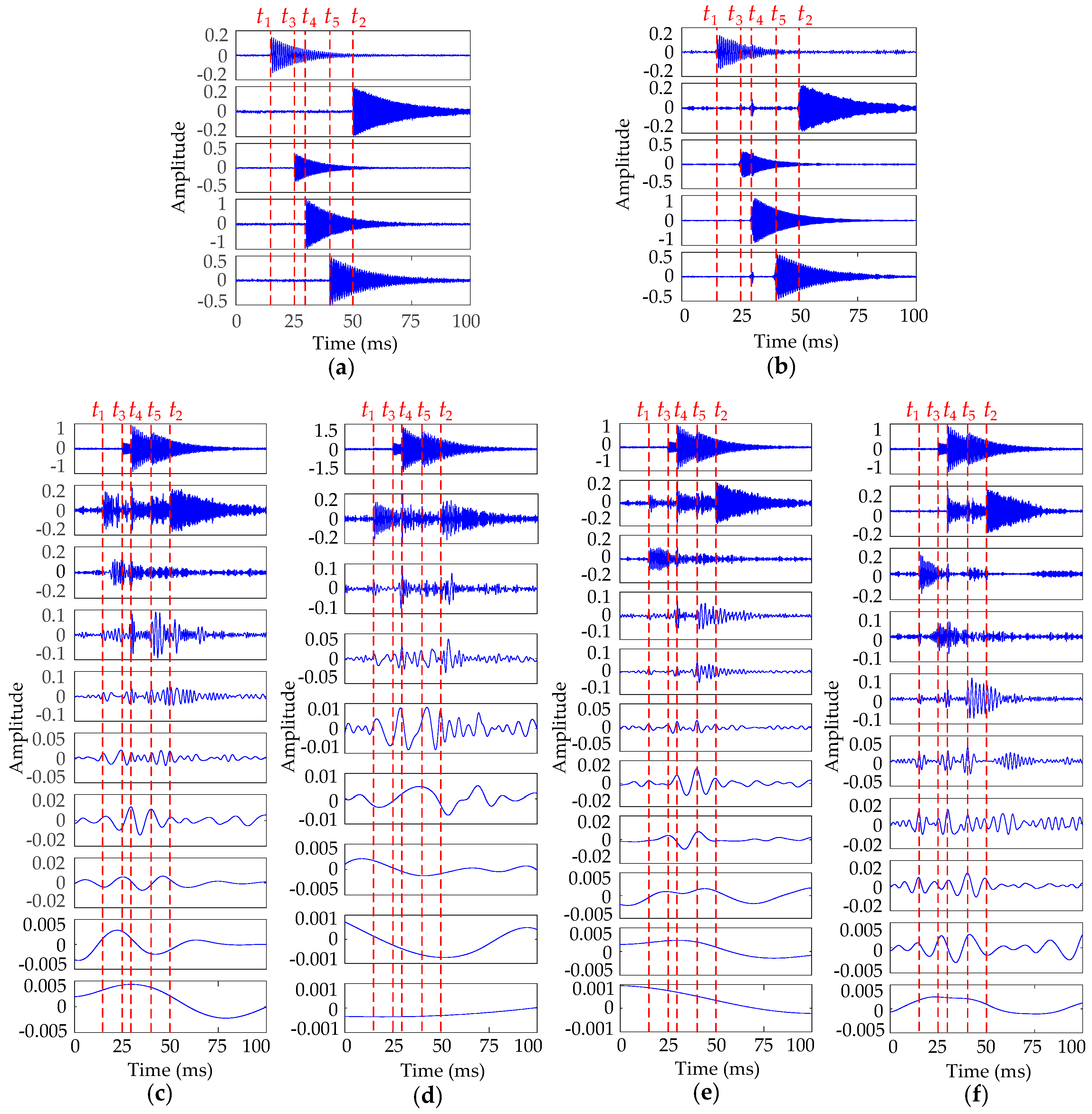
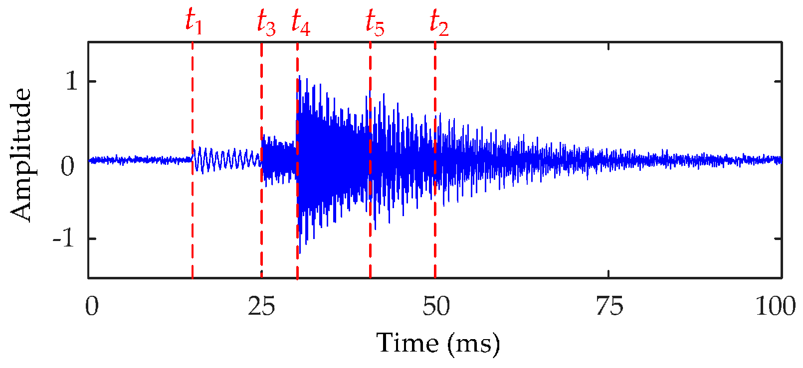
3.2. Simulated Vibration Signal Analysis Based on VMD
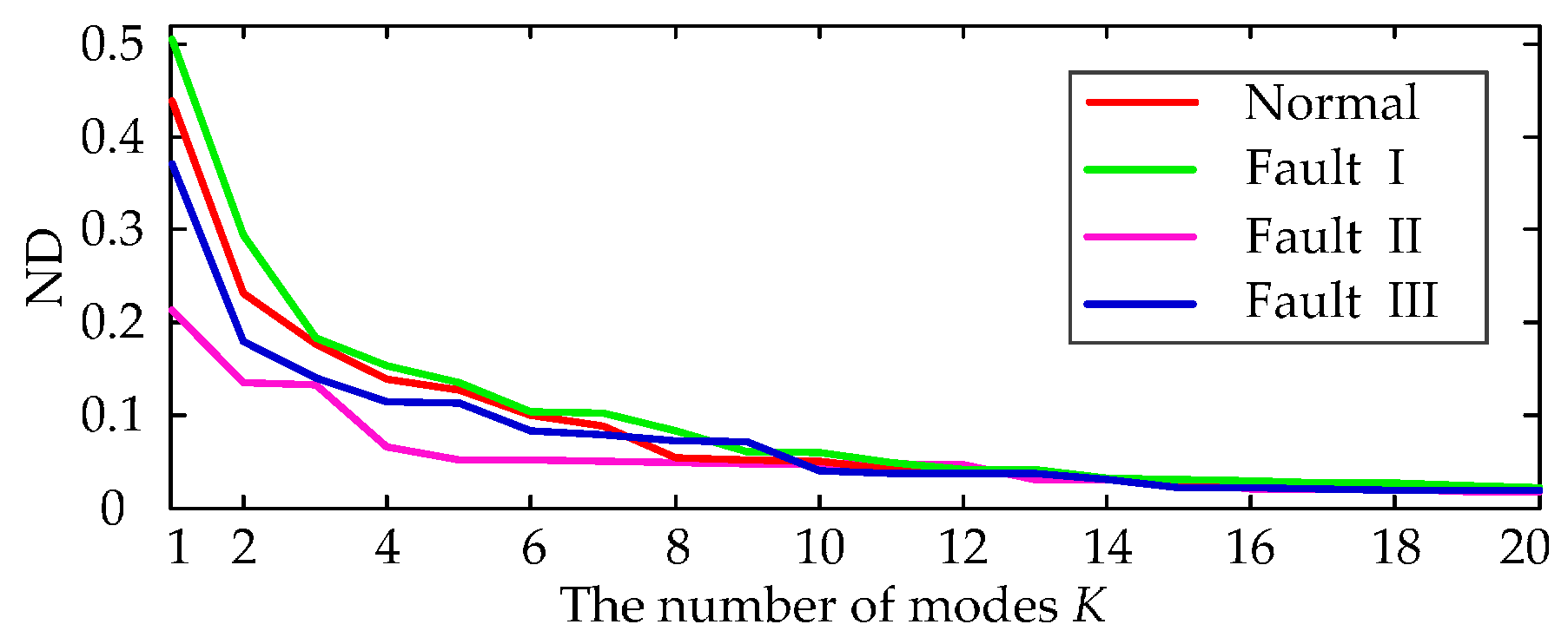
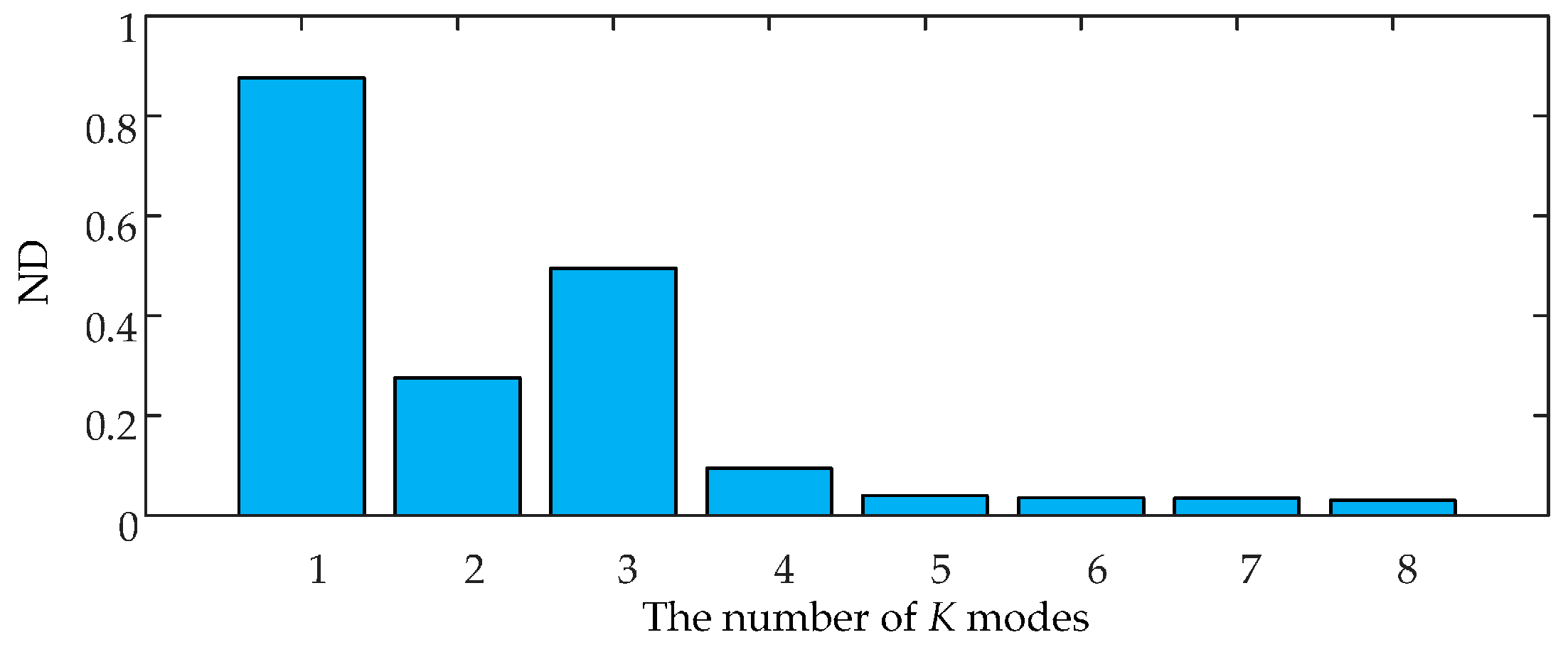
3.3. Determining the Number of K Modes of VMD
4. Principles of SVM and OCSVM
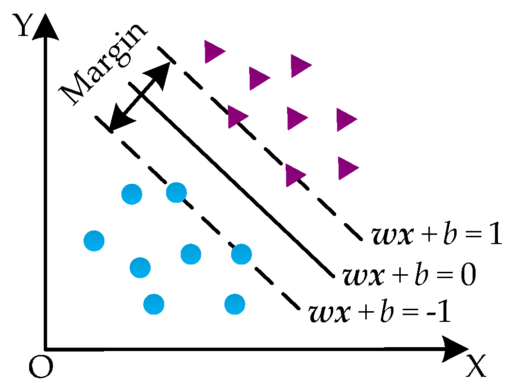
4.1. SVM
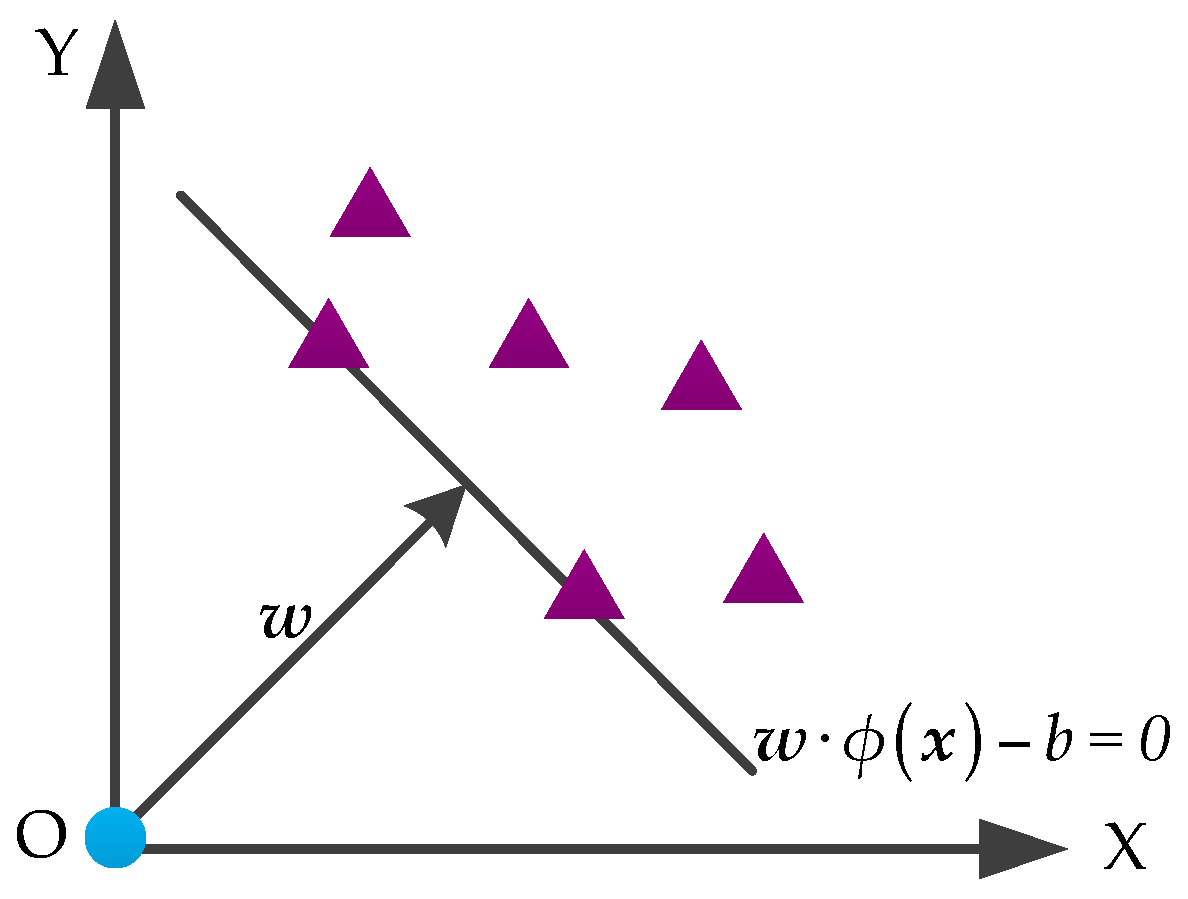
4.2. OCSVM
5. Feature Extraction of Vibration Signal
5.1. Singular Value Decomposition (SVD)
5.2. Feature Extraction Based on LSVD
- (1)
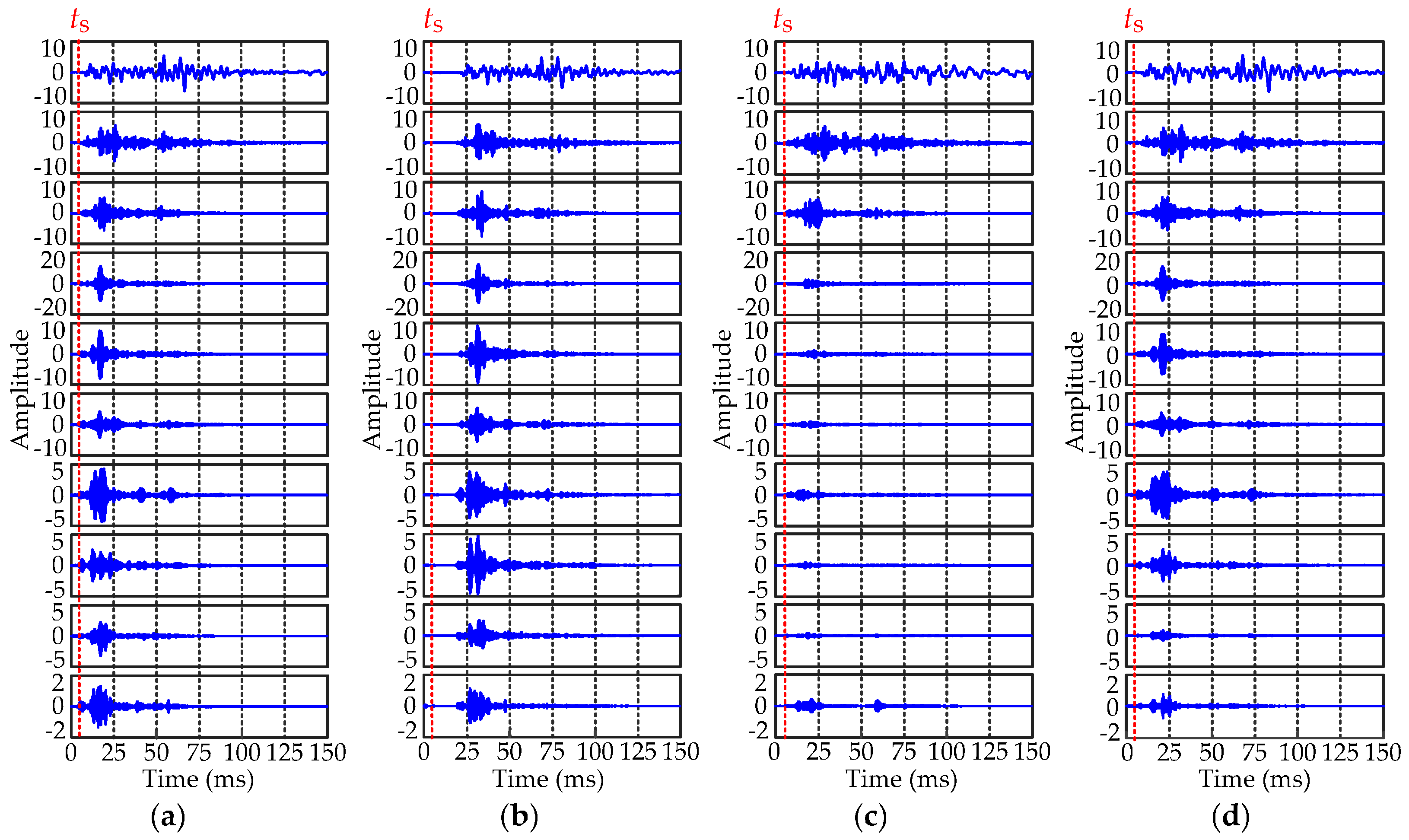
- VMD is used for decomposing HVCB vibration signals to obtain the IMF matrix.
- (2)
- The IMF matrix is equally divided into 30 submatrices along the time axis. The size of each submatrix is .
- (3)
- The 30 submatrices are decomposed by a series of SVDs, obtaining 30 singular value sequences.
- (4)
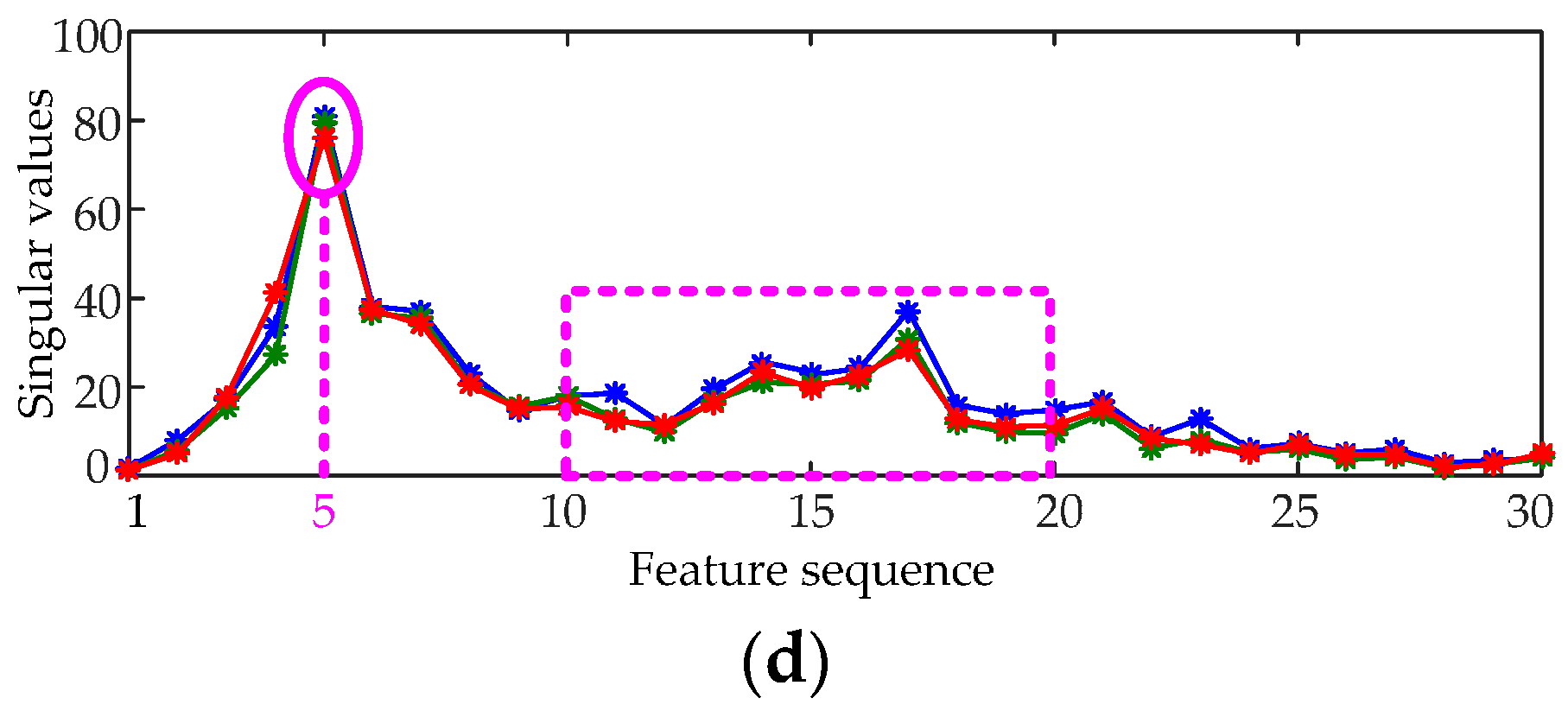
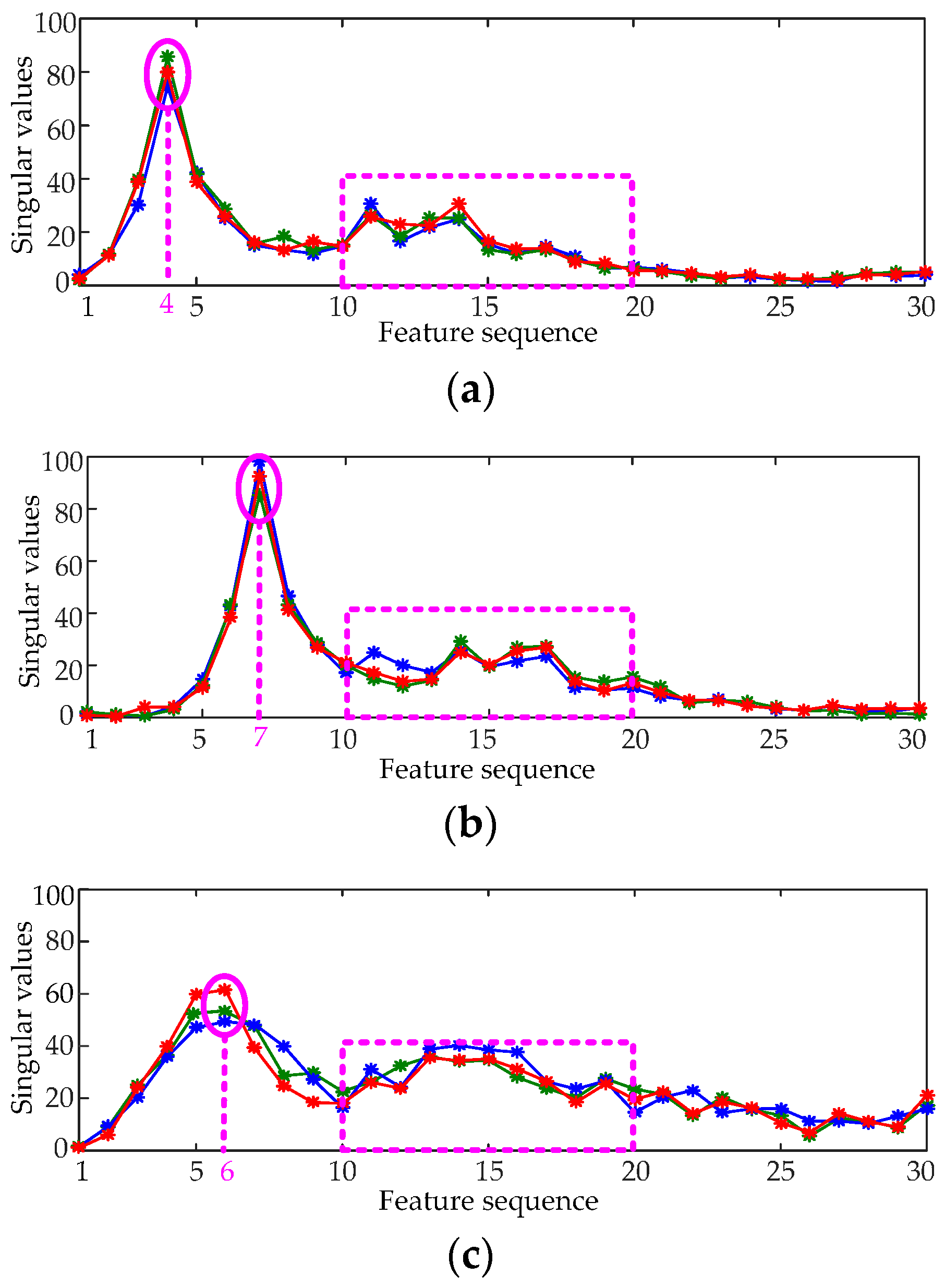
- The singular values of each submatrix attenuate rapidly; thus the largest singular value of each submatrix λimax is selected to construct the feature vector .
6. Experimental Results
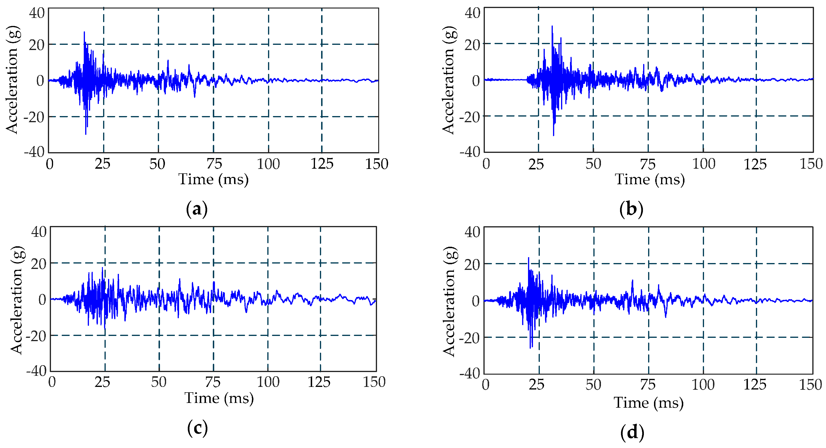
6.1. Feature Analysis of Measured Vibration Signal
6.2. Fault Classification Using MLC
7. Conclusions
- (1)
- Compared with EMD, the mode decomposed by VMD has a clearer physical meaning. The latter can reduce the influence of false modes for feature extraction and has a better property of feature presentation for vibration signals.
- (2)
- LSV can characterize the local and detailed features of vibration signals accurately, and the fault signatures can be extracted more precisely using the LSVD method, especially for delay fault.
- (3)
- MLC uses OCSVM to improve the ability to detect fault conditions. This method can identify unknown fault types. The diagnosis accuracy and the reliability of MLC are significantly enhanced compared with those of the SVM method.
Acknowledgments
Author Contributions
Conflicts of Interest
Appendix A
References
- CIGRE Working Group. Final Report of the Second International Enquiry on High Voltage Circuit Breaker Failures and Defects in Service; CIGRE Report No. 83; CIGRE: Paris, France, 1994. [Google Scholar]
- Runde, M.; Ottesen, G.E.; Skyberg, B.; Ohlen, M. Vibration analysis for diagnostic testing of circuit-breakers. IEEE Trans. Power Deliv. 1996, 11, 1816–1823. [Google Scholar] [CrossRef]
- Lee, D.S.; Lithgow, B.; Morrison, R.E. New fault diagnosis of circuit breakers. IEEE Trans. Power Deliv. 2003, 22, 61–61. [Google Scholar] [CrossRef]
- Landry, M.; Leonard, F.; Landry, C.; Beauchemin, R. An improved vibration analysis algorithm as a diagnostic tool for detecting mechanical anomalies on power circuit breakers. IEEE Trans. Power Deliv. 2008, 23, 1986–1994. [Google Scholar] [CrossRef]
- Meng, Y.P.; Jia, S.L.; Shi, Z.Q.; Rong, M.Z. The detection of the closing moments of a vacuum circuit breaker by vibration analysis. IEEE Trans. Power Deliv. 2006, 21, 652–658. [Google Scholar] [CrossRef]
- Huang, J.; Hu, X.G.; Yang, F. Support vector machine with genetic algorithm for machinery fault diagnosis of high voltage circuit breaker. Measurement 2011, 44, 1018–1027. [Google Scholar] [CrossRef]
- Huang, J.; Hu, X.G.; Geng, X. An intelligent fault diagnosis method of high voltage circuit breaker based on improved EMD energy entropy and multi-class support vector machine. Electr. Power Syst. Res. 2011, 81, 400–407. [Google Scholar] [CrossRef]
- Høidalen, H.K.; Runde, M. Continuous monitoring of circuit-breakers using vibration analysis. IEEE Trans. Power Deliv. 2005, 20, 2458–2465. [Google Scholar] [CrossRef]
- Huang, N.; Fang, L.; Cai, G.; Xu, D.; Chen, H.; Nie, Y. Mechanical Fault Diagnosis of High Voltage Circuit Breakers with Unknown Fault Type Using Hybrid Classifier Based on LMD and Time Segmentation Energy Entropy. Entropy 2016, 18, 322. [Google Scholar] [CrossRef]
- Sekiya, H.; Kimura, K.; Miki, C. Technique for determining bridge displacement response using MEMS accelerometers. Sensors 2016, 16, 257. [Google Scholar] [CrossRef] [PubMed]
- Flett, J.; Bone, G.M. Fault detection and diagnosis of diesel engine valve trains. Mech. Syst. Signal Process. 2015, 20, 316–327. [Google Scholar] [CrossRef]
- Harris, F.J. On the use of harmonic analysis with the discrete Fourier transform. Proc. IEEE 1978, 66, 51–83. [Google Scholar] [CrossRef]
- Zhu, K.; Wong, Y.S.; Hong, G.S. Wavelet analysis of sensor signals for tool condition monitoring: A review and some new results. Int. J. Mach. Tool. Manuf. 2009, 49, 537–553. [Google Scholar] [CrossRef]
- Peng, Z.K.; Jackson, M.R.; Rongong, J.A.; Chu, F.L.; Parkin, R.M. On the energy leakage of discrete wavelet transform. Mech. Syst. Signal Process. 2009, 23, 330–343. [Google Scholar] [CrossRef]
- Huang, N.E.; Shen, Z.; Long, S.R.; Wu, M.C.; Shih, H.H.; Zheng, Q.; Yen, N.C.; Tung, C.C.; Liu, H.H. The empirical mode decomposition and the Hilbert spectrum for nonlinear and non-stationary time series analysis. Proc. R. Soc. A-Math. Phys. Eng. 1998, 454, 903–995. [Google Scholar] [CrossRef]
- Dragomiretskiy, K.; Zosso, D. Variational mode decomposition. IEEE Trans. Signal Process. 2014, 62, 531–544. [Google Scholar] [CrossRef]
- Yin, A.J.; Ren, H.J. A propagating mode extraction algorithm for microwave waveguide using variational mode decomposition. Meas. Sci. Technol. 2015, 26. [Google Scholar] [CrossRef]
- Abdoos, A.A.; Mianaei, P.K.; Ghadikolaei, M.R. Combined VMD-SVM based feature selection method for classification of power quality events. Appl. Soft Comput. 2015, 38, 637–646. [Google Scholar] [CrossRef]
- Upadhyay, A.; Pachori, R.B. Instantaneous voiced/non-voiced detection in speech signals based on variational mode decomposition. J. Frankl. Inst. 2015, 352, 2679–2707. [Google Scholar] [CrossRef]
- Wang, Y.X.; Markert, R.; Xiang, J.W.; Zheng, W.G. Research on variational mode decomposition and its application in detecting rub-impact fault of the rotor system. Mech. Syst. Signal Process. 2015, 60, 243–251. [Google Scholar] [CrossRef]
- Tayarani-Bathaie, S.S.; Khorasani, K. Fault detection and isolation of gas turbine engines using a bank of neural networks. J. Process Control 2015, 36, 22–41. [Google Scholar] [CrossRef]
- Paliwal, M.; Kumar, U.A. Neural networks and statistical techniques: A review of applications. Expert Syst. Appl. 2009, 36, 2–17. [Google Scholar] [CrossRef]
- Xian, G.M.; Zeng, B.Q. An intelligent fault diagnosis method based on wavelet packer analysis and hybrid support vector machines. Expert Syst. Appl. 2009, 37, 12131–12136. [Google Scholar] [CrossRef]
- Schölkopf, B.; Platt, J.C.; Shawe-Taylor, J.; Smola, A.J.; Williamson, R.C. Estimating the support of a high-dimensional distribution. Neural Comput. 2001, 13, 1443–1471. [Google Scholar] [CrossRef] [PubMed]
- Huang, N.T.; Chen, H.J.; Zhang, S.X.; Cai, G.W.; Li, W.G.; Xu, D.G.; Fang, L.H. Mechanical Fault Diagnosis of High Voltage Circuit Breakers Based on Wavelet Time-Frequency Entropy and One-Class Support Vector Machine. Entropy 2016, 18, 7. [Google Scholar] [CrossRef]
- Mahadevan, S.; Shah, S.L. Fault detection and diagnosis in process data using one-class support vector machines. J. Process Control 2009, 19, 1627–1639. [Google Scholar] [CrossRef]
- Fernández-Francos, D.; Martínez-Rego, D.; Fontenla-Romero, O.; Alonso-Betanzos, A. Automatic bearing fault diagnosis based on one-class v-SVM. Comput. Ind. Eng. 2013, 64, 357–365. [Google Scholar] [CrossRef]
- Yin, S.; Zhu, X.P.; Jing, C. Fault detection based on a robust one class support vector machine. Neurocomputing 2014, 145, 263–268. [Google Scholar] [CrossRef]
- Bertsekas, D.P. Multiplier methods: A survey. Automatica 1976, 12, 133–145. [Google Scholar] [CrossRef]
- Wu, Z.H.; Huang, N.E. Ensemble empirical mode decomposition: A noise-assisted data analysis method. Adv. Adapt. Data Anal. 2011, 1, 1–41. [Google Scholar] [CrossRef]
- Torres, M.E.; Colominas, M.A.; Schlotthauer, G.; Flandrin, P. A complete ensemble empirical mode decomposition with adaptive noise. In Proceedings of the 2011 IEEE International Conference on Acoustics, Speech and Signal Processing (ICASSP), Prague, Czech Republic, 22–27 May 2011.
- Vapnik, V.N. The Nature of Statistical Learning Theory, 1st ed.; Springer: New York, NY, USA, 1995; pp. 127–140. [Google Scholar]
- Klema, V.C.; Laub, A.J. The singular value decomposition: its computation and some applications. IEEE Trans. Autom. Control 1980, 25, 164–176. [Google Scholar] [CrossRef]
- Tian, Y.; Tan, T.N.; Wang, Y.H.; Fang, Y.C. Do singular values contain adequate information for face recognition. Pattern Recognit. 2003, 36, 649–655. [Google Scholar] [CrossRef]
- Tian, Y.; Ma, J.; Lu, C.; Wang, Z.L. Rolling bearing fault diagnosis under variable conditions using LMD-SVD and extreme learning machine. Mech. Mach. Theory 2015, 90, 175–186. [Google Scholar] [CrossRef]


| Vibration Events | Ai | ti (ms) | fi (Hz) | μi |
|---|---|---|---|---|
| V1 | 0.15 | 15 | 1200 | 80 |
| V2 | 0.2 | 50 | 3000 | 50 |
| V3 | 0.3 | 25 | 4500 | 95 |
| V4 | 1.0 | 30 | 5500 | 75 |
| V5 | 0.5 | 40 | 7000 | 60 |
| Classifier | Test Sample | Diagnosis Results | Accuracy | ||||
|---|---|---|---|---|---|---|---|
| Normal | Fault I | Fault II | Fault III | New Fault | |||
| MLC | Normal | 18 | 0 | 0 | 2 | 0 | 90% |
| Fault I | 0 | 20 | 0 | 0 | 0 | 100% | |
| Fault II | 0 | 0 | 20 | 0 | 0 | 100% | |
| Fault III | 0 | 0 | 0 | 20 | 0 | 100% | |
| SVM | Normal | 19 | 0 | 0 | 1 | - | 95% |
| Fault I | 0 | 20 | 0 | 0 | - | 100% | |
| Fault II | 0 | 0 | 20 | 0 | - | 100% | |
| Fault III | 3 | 0 | 0 | 17 | - | 85% | |
| Classifier | Test Sample | Diagnosis Results | Accuracy | ||||
|---|---|---|---|---|---|---|---|
| Normal | Fault I | Fault II | Fault III | New Fault | |||
| MLC | Normal | 14 | 6 | 0 | 0 | 0 | 70% |
| Fault I | 5 | 15 | 0 | 0 | 0 | 75% | |
| Fault II | 0 | 0 | 19 | 0 | 1 | 95% | |
| Fault III | 0 | 3 | 0 | 17 | 0 | 85% | |
| SVM | Normal | 13 | 7 | 0 | 0 | - | 65% |
| Fault I | 8 | 11 | 0 | 1 | - | 55% | |
| Fault II | 0 | 0 | 20 | 0 | - | 100% | |
| Fault III | 3 | 2 | 0 | 15 | - | 70% | |
| Classifier | Diagnosis Results | Accuracy | |||
|---|---|---|---|---|---|
| Normal | Fault I | Fault II | New Fault | ||
| MLC | 0 | 0 | 0 | 20 | 100% |
| SVM | 20 | 0 | 0 | - | 0 |
© 2016 by the authors; licensee MDPI, Basel, Switzerland. This article is an open access article distributed under the terms and conditions of the Creative Commons Attribution (CC-BY) license (http://creativecommons.org/licenses/by/4.0/).
Share and Cite
Huang, N.; Chen, H.; Cai, G.; Fang, L.; Wang, Y. Mechanical Fault Diagnosis of High Voltage Circuit Breakers Based on Variational Mode Decomposition and Multi-Layer Classifier. Sensors 2016, 16, 1887. https://doi.org/10.3390/s16111887
Huang N, Chen H, Cai G, Fang L, Wang Y. Mechanical Fault Diagnosis of High Voltage Circuit Breakers Based on Variational Mode Decomposition and Multi-Layer Classifier. Sensors. 2016; 16(11):1887. https://doi.org/10.3390/s16111887
Chicago/Turabian StyleHuang, Nantian, Huaijin Chen, Guowei Cai, Lihua Fang, and Yuqiang Wang. 2016. "Mechanical Fault Diagnosis of High Voltage Circuit Breakers Based on Variational Mode Decomposition and Multi-Layer Classifier" Sensors 16, no. 11: 1887. https://doi.org/10.3390/s16111887
APA StyleHuang, N., Chen, H., Cai, G., Fang, L., & Wang, Y. (2016). Mechanical Fault Diagnosis of High Voltage Circuit Breakers Based on Variational Mode Decomposition and Multi-Layer Classifier. Sensors, 16(11), 1887. https://doi.org/10.3390/s16111887