
Indoor-Outdoor Detection Using a Smart Phone Sensor

Abstract
:1. Introduction
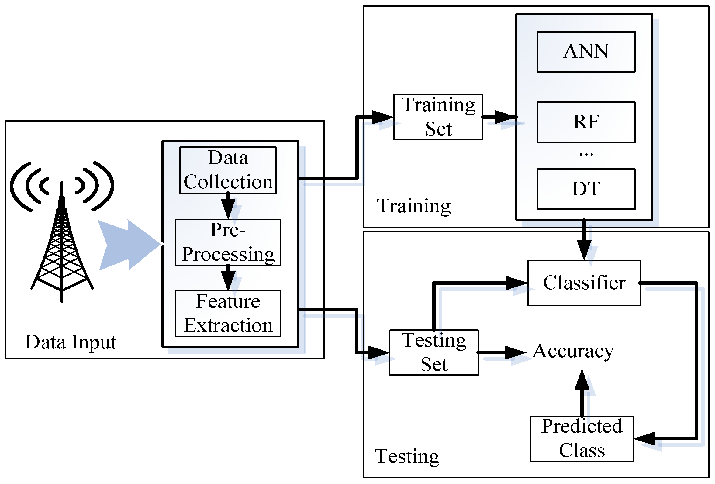
2. Methodology
2.1. Data Input
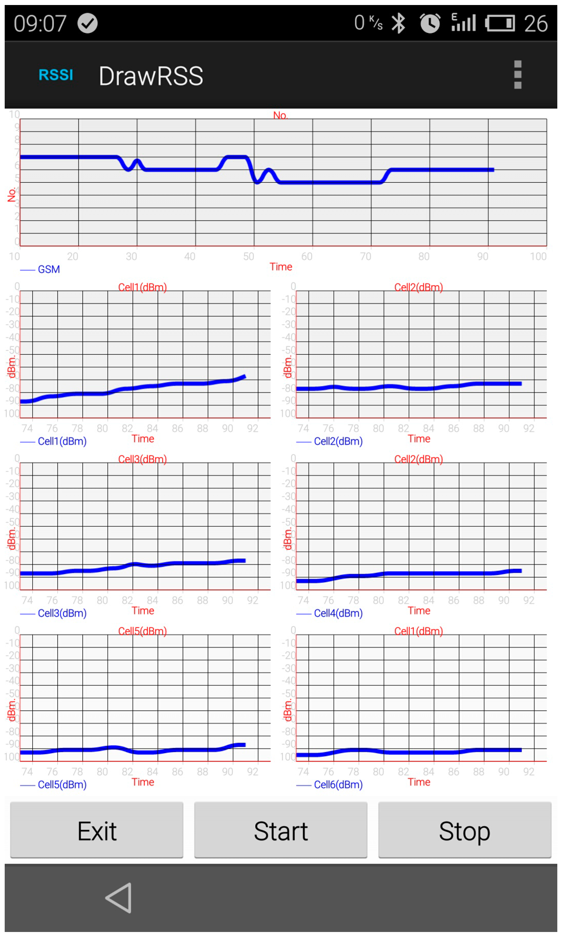
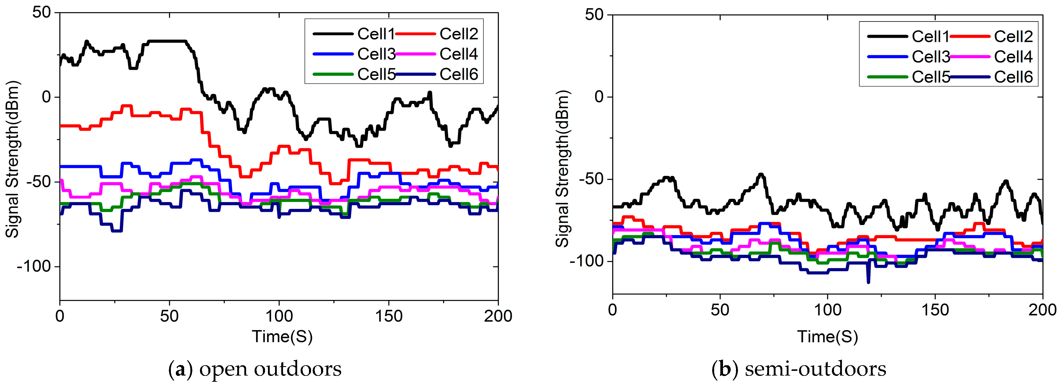
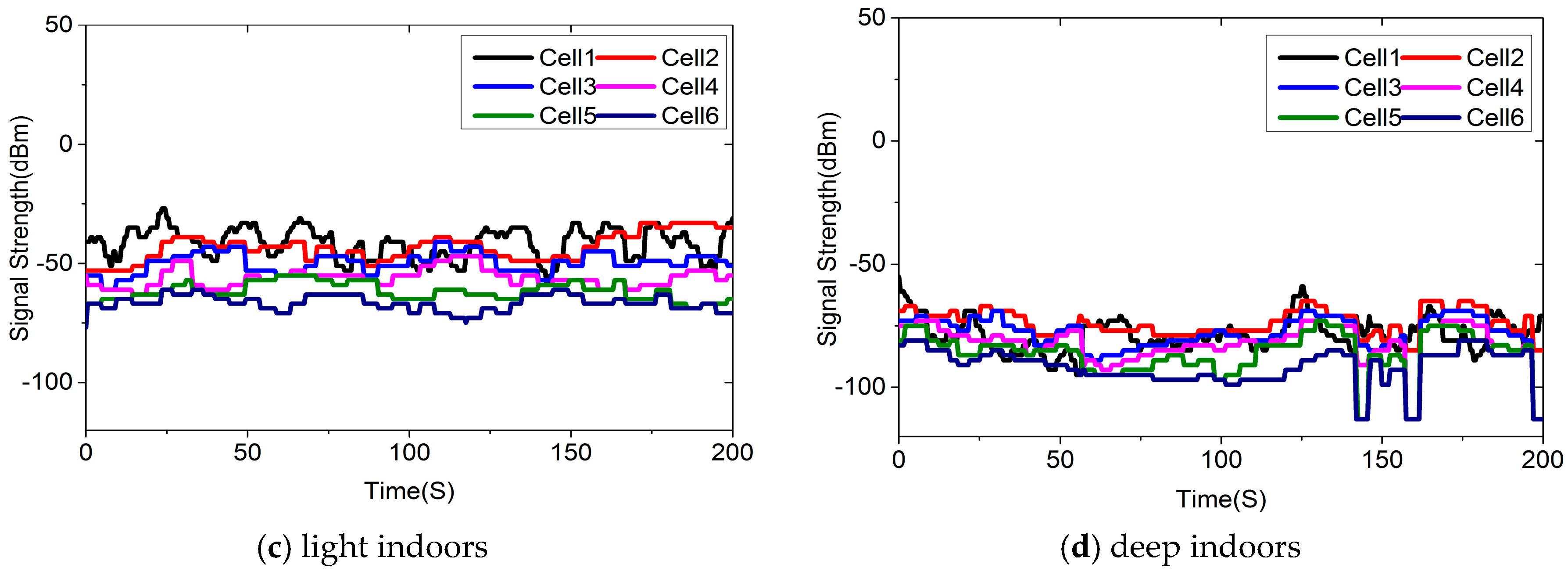
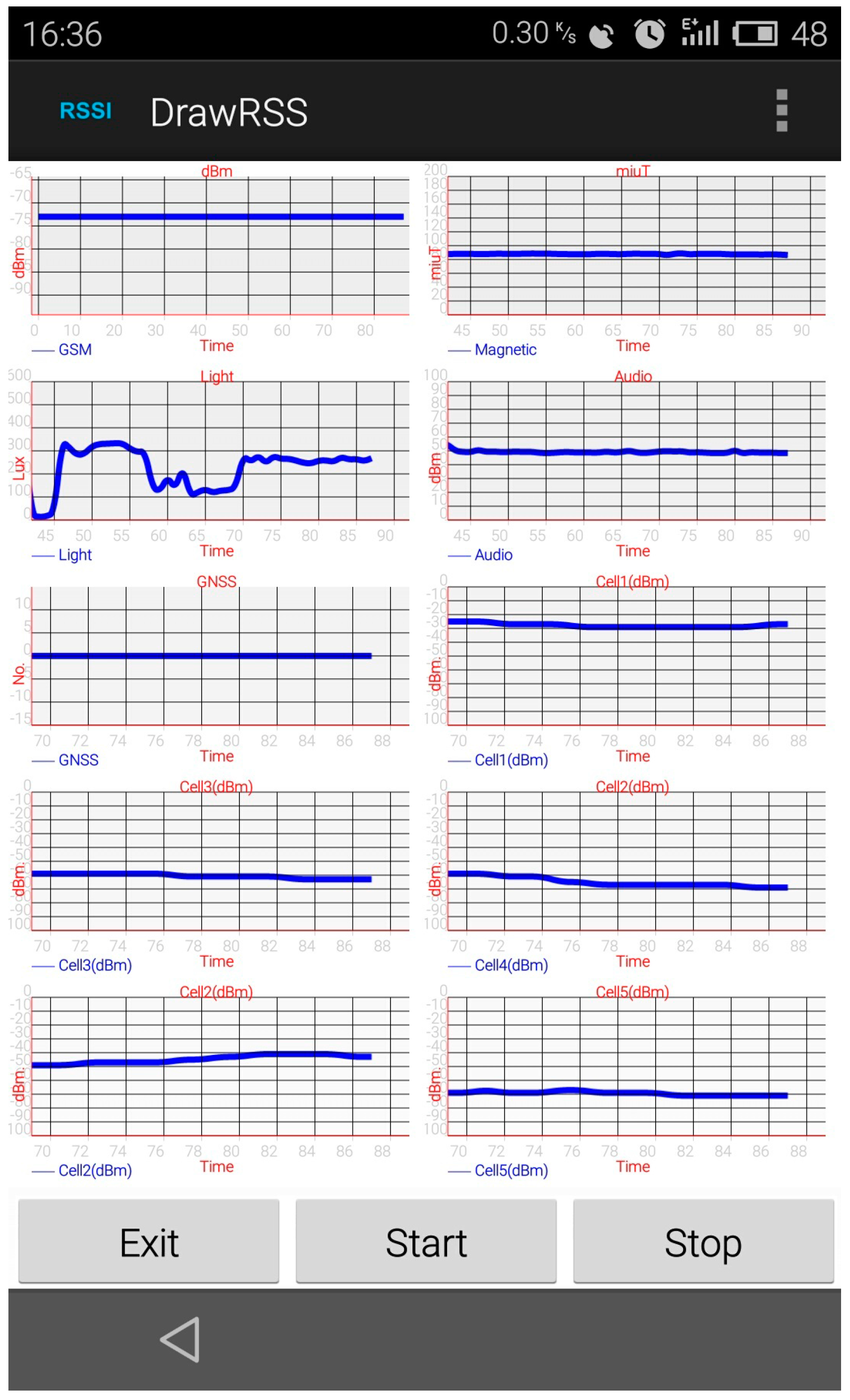
2.1.1. Data Collection
2.1.2. Data Pre-Processing
2.1.3. Feature Extraction
- (1)
- MeanMean is the most basic character of a signal. It is calculated by summing the values and dividing the numbers:where |*| is the number getting operation. Mean is a measure of the middle value of a signal.
- (2)
- Standard DeviationStandard Deviation is an indicator of how much a signal is dispersed around its mean. It is calculated as follows:
- (3)
- Maximum and MinimumMaximum and Minimum values are the extreme values in the window:
- (4)
- RangeRange is the difference between the Maximum and Minimum values:
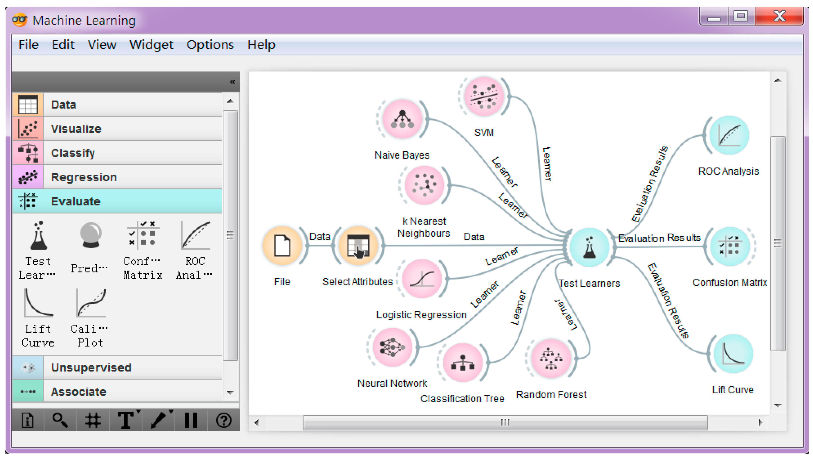
2.2. Training
2.3. Testing
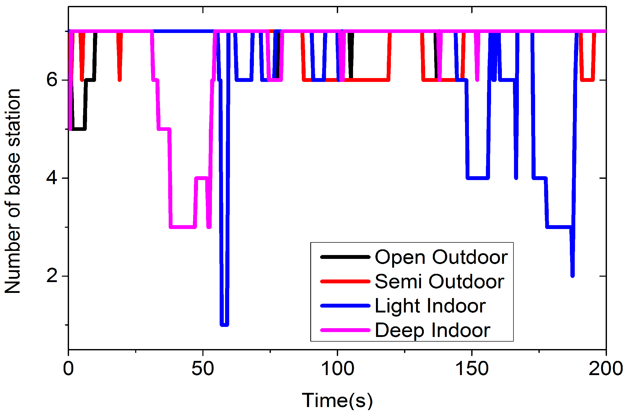
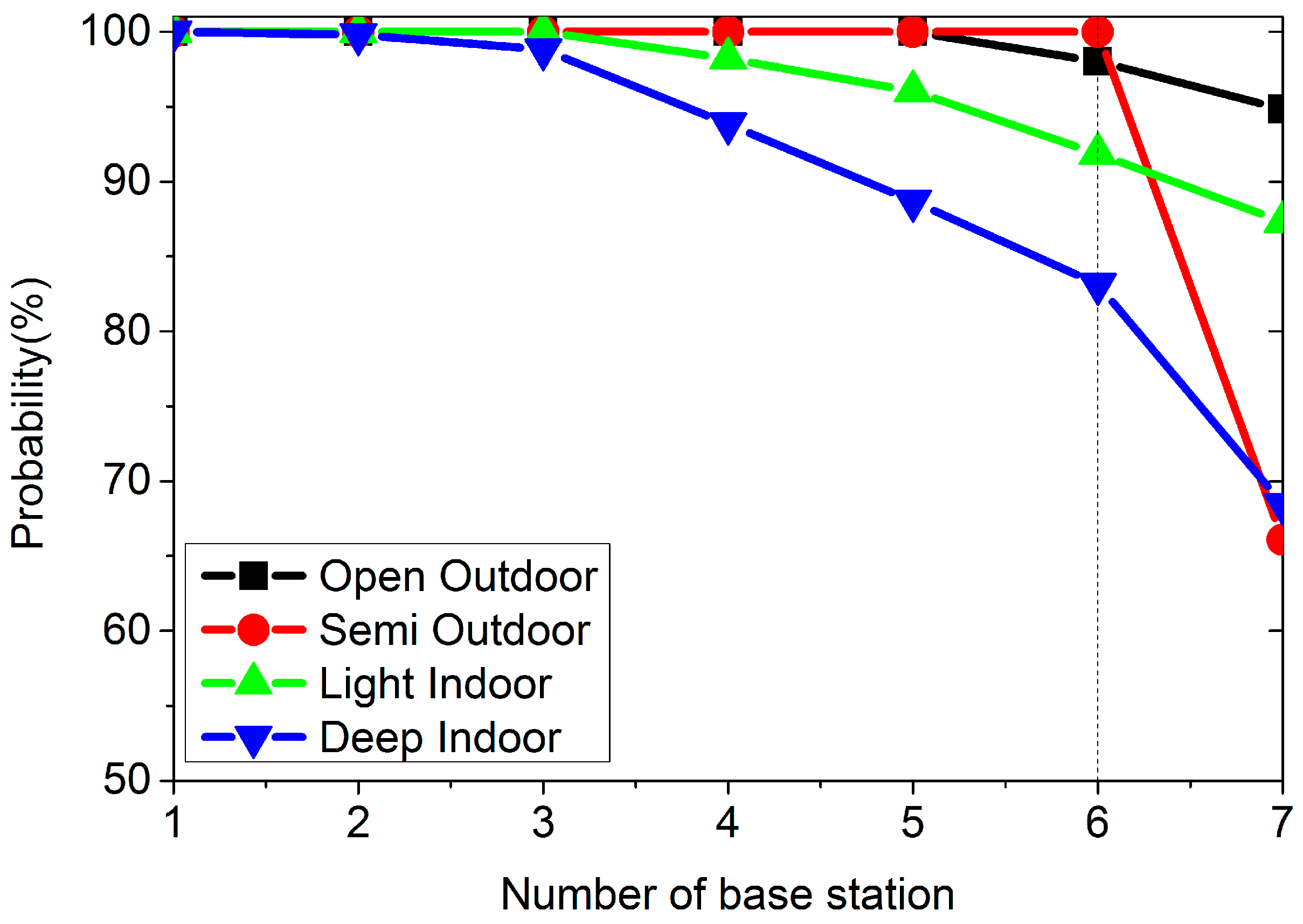
3. Experiments
4. Data Analysis
5. Discussion and Conclusions
Supplementary Materials
Acknowledgments
Author Contributions
Conflicts of Interest
References
- Groves, P.D. Shadow matching: A new GNSS positioning technique for urban canyons. J. Navig. 2011, 64, 417–430. [Google Scholar] [CrossRef]
- Cheng, J.; Yang, L.; Li, Y.; Zhang, W. Seamless outdoor/indoor navigation with WIFI/GPS aided low cost Inertial Navigation System. Phys. Commun. 2014, 13, 31–43. [Google Scholar] [CrossRef]
- Li, M.; Zhou, P.; Zheng, Y. IODetector: A Generic Service for Indoor/Outdoor Detection. ACM Trans. Sens. Netw. 2014, 11. [Google Scholar] [CrossRef]
- Dadu, V.; Katasikouli, P.; Sarkar, R.; Marina, M.K. A Semi-Supervised Learning Approach for Robust Indoor-Outdoor Detection with Smartphones. In Proceedings of the 12th ACM Conference on Embedded Network Sensor Systems, Memphis, TN, USA, 3–6 November 2014.
- Kaplan, E.D. Understanding GPS: Principles and Applications; Artech House: London, UK, 2005. [Google Scholar]
- Caceres, M.A.; Penna, F.; Wymeersch, H.; Garello, R. Hybrid cooperative positioning based on distributed belief propagation. IEEE J. Sel. Areas Commun. 2011, 29, 1948–1958. [Google Scholar] [CrossRef]
- Chen, W.; Wang, W.; Li, Q.; Chang, Q.; Hou, H. A Crowd-Sourcing Indoor Localization Algorithm via Optical Camera on a Smartphone Assisted by Wi-Fi Fingerprint RSSI. Sensors 2016, 16, 410. [Google Scholar] [CrossRef] [PubMed]
- Bahl, P.; Padmanabhan, V.N. RADAR: An in-building RF-based user location and tracking system. In Proceedings of Nineteenth Annual Joint Conference of the IEEE Computer and Communications Societies, Tel Aviv, Israel, 26–30 March 2000.
- Walter, D.J.; Groves, P.D.; Mason, R.J.; Harrison, J.; Woodward, J.; Wright, P. Novel Environmental Features for Robust Multisensor Navigation. In Proceedings of the 26th International Technical Meeting of the Satellite Division of the Institute of Navigation (ION GNSS 2013), Nashville, TN, USA, 16–20 September 2013.
- Groves, P.D.; Martin, H.F.S.; Voutsis, K.; Walter, D.J.; Wang, L. Context detection, categorization and connectivity for advanced adaptive integrated navigation. In Proceedings of the 26th International Technical Meeting of the Satellite Division of the Institute of Navigation (ION GNSS 2013), Nashville, TN, USA, 16–20 September 2013.
- Muralidharan, K.; Khan, A.J.; Misra, A.; Balan, R.K.; Agarwal, S. Barometric phone sensors: More hype than hope! In Proceedings of the 15th Workshop on Mobile Computing Systems and Applications, Santa Barbara, CA, USA, 26–27 February 2014.
- Ravindranath, L.; Newport, C.; Balakrishnan, H.; Madden, S. Improving wireless network performance using sensor hints. In Proceedings of the 8th USENIX Conference on Networked Systems Design and Implementation, Boston, MA, USA, 30 March–1 April 2011.
- Liu, J.; Priyantha, B.; Hart, T.; Ramos, H.S.; Loureiro, A.A.F.; Wang, Q. Energy efficient GPS sensing with cloud offloading. In Proceedings of the 10th ACM Conference on Embedded Network Sensor Systems, Toronto, ON, Canada, 6–9 November 2012; pp. 85–98.
- Lin, K.; Kansal, A.; Lymberopoulos, D.; Zhao, F. Energy-accuracy trade-off for continuous mobile device location. In Proceedings of the 8th International Conference on Mobile Systems, Applications, and Services, San Francisco, CA, USA, 15–18 June 2010; pp. 285–298.
- Elhoushi, M.; Georgy, J.; Wahdan, A.; Korenberg, M.; Noureldin, A. Using portable device sensors to recognize height changing modes of motion. In Proceedings of the 2014 IEEE International Instrumentation and Measurement Technology Conference (I2MTC), Montevideo, Uruguay, 12–15 May 2014; pp. 477–481.
- Elhoushi, M. Advanced Motion Mode Recognition for Portable Navigation. Ph.D. Thesis, Queen’s University, Kingston, ON, Canada, 2015. [Google Scholar]
- Elhoushi, M.; Georgy, J.; Korenberg, M.; Noureldin, A. Robust motion mode recognition for portable navigation independent on device usage. In Proceedings of the 2014 IEEE/ION Position, Location and Navigation Symposium (PLANS 2004), Monterey, CA, USA, 5–8 May 2014; pp. 158–163.
- Vanini, S.; Giordano, S. Adaptive context-agnostic floor transition detection on smart mobile devices. In Proceedings of the 2013 IEEE International Conference on Pervasive Computing and Communications Workshops (PERCOM Workshops), San Diego, CA, USA, 18–22 March 2013; pp. 2–7.
- Krumm, J.; Hariharan, R. TempIO: Inside/outside classification with temperature. In Proceedings of the 2nd Workshop on Man-Machine Symbiotic Systems, Kyoto, Japan, 23–24 November 2004.
- Wu, M.; Pathak, P.H.; Mohapatra, P. Monitoring building door events using barometer sensor in smartphones. In Proceedings of the 2015 ACM International Joint Conference on Pervasive and Ubiquitous Computing, Osaka, Japan, 7–11 September 2015; pp. 319–323.
- Ergen, S.C.; Tetikol, H.S.; Kontik, M.; Sevlian, R.; Rajagopal, R.; Varaiya, P. RSSI-fingerprinting-based mobile phone localization with route constraints. IEEE Trans. Veh. Technol. 2014, 63, 423–428. [Google Scholar] [CrossRef]
- Chen, R.; Chu, T.; Liu, K.; Liu, J.; Chen, Y. Inferring Human Activity in Mobile Devices by Computing Multiple Contexts. Sensors 2015, 15, 21219–21238. [Google Scholar] [CrossRef] [PubMed]
- Rappaport, T.S. Wireless Communications: Principles and Practice; Prentice Hall PTR: Upper Saddle River, NJ, USA, 1996; Volume 2. [Google Scholar]
- Orange. Available online: http://www.ailab.si/orange/ (accessed on 3 March 2016).
- Stanivuk, V. Measurements of the GSM signal strength by mobile phone. In Proceedings of the 2012 20th Telecommunications Forum (TELFOR), Belgrade, Serbia, 20–22 November 2012; pp. 1784–1787.
- Kyritsi, P.; Cox, D.C. Propagation characteristics of horizontally and vertically polarized electric fields in an indoor environment: Simple model results. In Proceedings of the IEEE 54th Vehicular Technology Conference VTC Fall 2001, Atlantic City, NJ, USA, 7–11 October 2001; Volume 3, pp. 1422–1426.


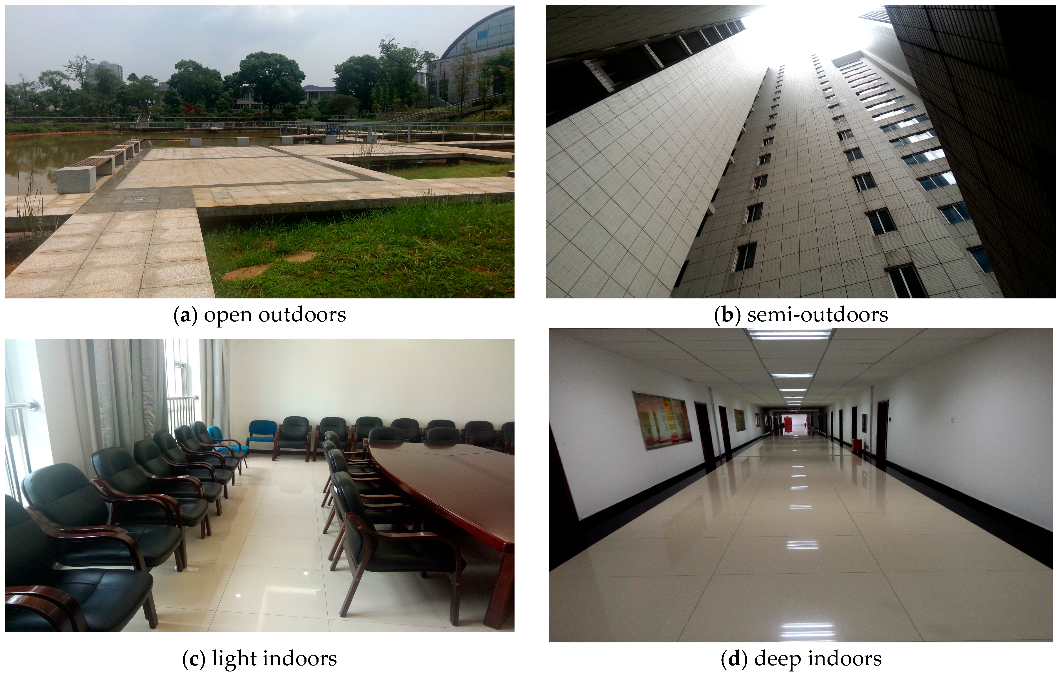
| Environment | Open Outdoors | Semi-Outdoors | Light Indoors | Deep Indoors |
|---|---|---|---|---|
| Definition | Outside a building | Near a building | In a room with windows | In a room without windows |
| Example |  |  |  |  |
| Class | Class 1 | Class 2 | Class 3 |
|---|---|---|---|
| Class 1 | n11 | n12 | n13 |
| Class 2 | n21 | n22 | n23 |
| Class 3 | n31 | n32 | n33 |
| Definition | Formula | |
|---|---|---|
| True Positive (TP) | The number of samples of a class which have been correctly classified | |
| True Negative (TN) | The number of samples of other classes which has been correctly classified | |
| False Positive (FP) | The number of samples not belongs to a class which has been incorrectly classified as belonging to it | |
| False Negative (FN) | The number of samples belonging to a class which have been incorrectly classified as belong to other class | |
| Accuracy | The proportion of all samples which have been correctly classified | |
| Sensitivity | The proportion of samples which have been correctly classified | |
| Precision | The proportion of sample predicted to belong to a class which is correct | |
| Specificity | The proportion of negative samples which have been correctly classified to be negative | |
| F-Measure | the weighted average of the precision and sensitivity |
| Environment | Deep Indoors | Semi-Outdoors | Light Indoors | Open Outdoors |
|---|---|---|---|---|
| Deep Indoors | 97.1% | 0 | 2.9% | 0 |
| Semi Outdoors | 0 | 98.6% | 0 | 1.4% |
| Light Indoors | 6.5% | 0 | 93.5% | 0 |
| Open Outdoors | 0 | 0 | 0 | 100% |
| Algorithm | Accuracy | Sensitivity | Specificity | F-Measure | Precision |
|---|---|---|---|---|---|
| SVM | 0.8095 | 0.8095 | 0.9365 | 0.8077 | 0.8087 |
| KNN | 0.8652 | 0.8652 | 0.9551 | 0.8638 | 0.8634 |
| DT | 0.8861 | 0.8861 | 0.9621 | 0.8856 | 0.8901 |
| NB | 0.8734 | 0.8734 | 0.9578 | 0.8719 | 0.8717 |
| LR | 0.7994 | 0.7994 | 0.9331 | 0.7932 | 0.8051 |
| NN | 0.8677 | 0.8677 | 0.9559 | 0.8658 | 0.8652 |
| RF | 0.8943 | 0.8943 | 0.9647 | 0.8938 | 0.8933 |
| Random Forest | IODetector | Co-Training | GPS | |
|---|---|---|---|---|
| Accuracy | 95.3% | 61.2% | 93.14% | 71.6% |
© 2016 by the authors; licensee MDPI, Basel, Switzerland. This article is an open access article distributed under the terms and conditions of the Creative Commons Attribution (CC-BY) license (http://creativecommons.org/licenses/by/4.0/).
Share and Cite
Wang, W.; Chang, Q.; Li, Q.; Shi, Z.; Chen, W. Indoor-Outdoor Detection Using a Smart Phone Sensor. Sensors 2016, 16, 1563. https://doi.org/10.3390/s16101563
Wang W, Chang Q, Li Q, Shi Z, Chen W. Indoor-Outdoor Detection Using a Smart Phone Sensor. Sensors. 2016; 16(10):1563. https://doi.org/10.3390/s16101563
Chicago/Turabian StyleWang, Weiping, Qiang Chang, Qun Li, Zesen Shi, and Wei Chen. 2016. "Indoor-Outdoor Detection Using a Smart Phone Sensor" Sensors 16, no. 10: 1563. https://doi.org/10.3390/s16101563
APA StyleWang, W., Chang, Q., Li, Q., Shi, Z., & Chen, W. (2016). Indoor-Outdoor Detection Using a Smart Phone Sensor. Sensors, 16(10), 1563. https://doi.org/10.3390/s16101563