
Learning to Rapidly Re-Contact the Lost Plume in Chemical Plume Tracing


Abstract
:1. Introduction
2. Background
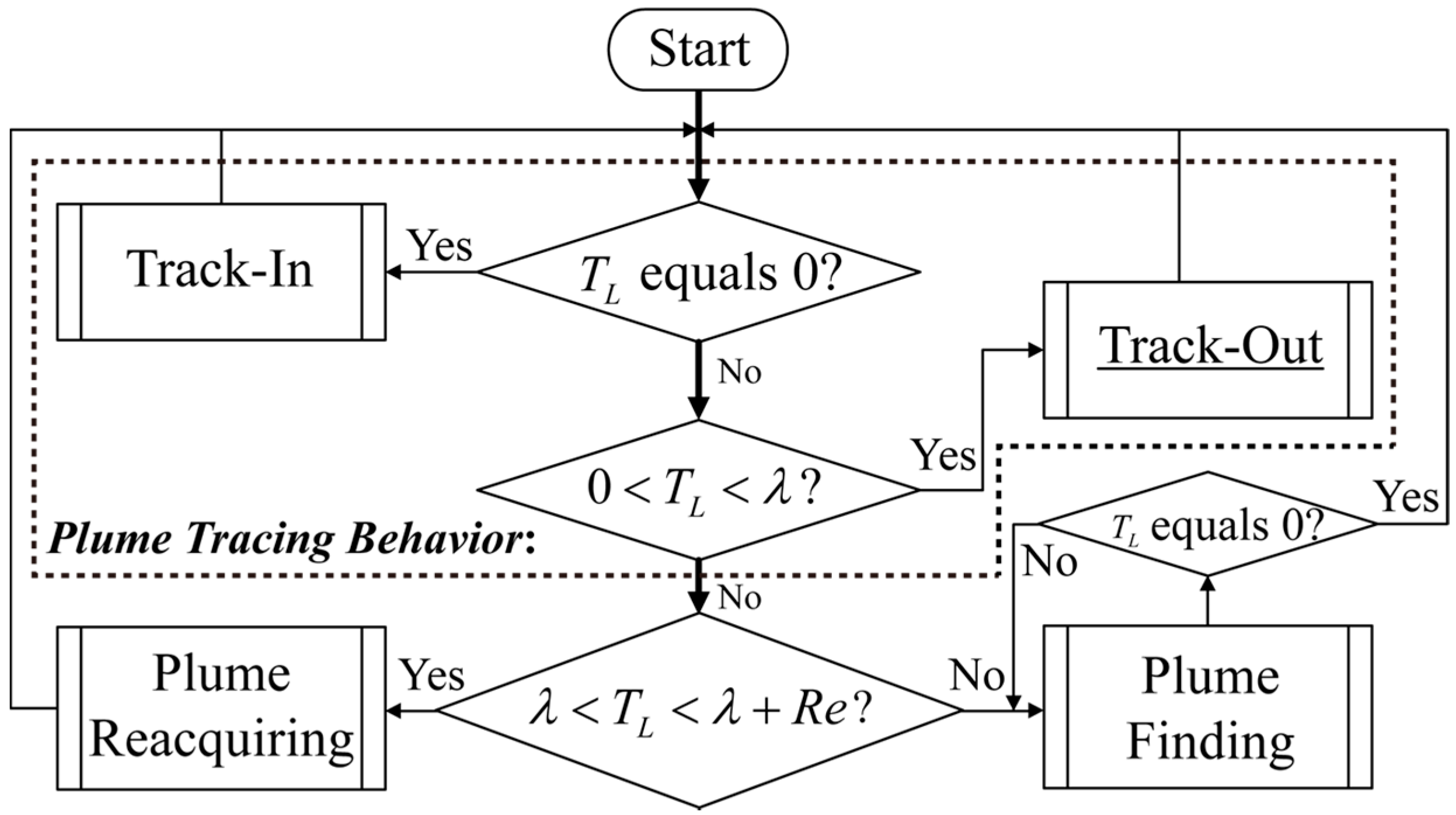
2.1. Track-Out Activity Using BUS

2.2. Reinforcement Learning
3. Learning to Re-Contact the Plume via VTF and cVTF
3.1. VTF Method
3.1.1. Preliminaries
Problem Formulation
Handling of the Continuous State and Action Spaces

3.1.2. Main Steps of the VTF Method
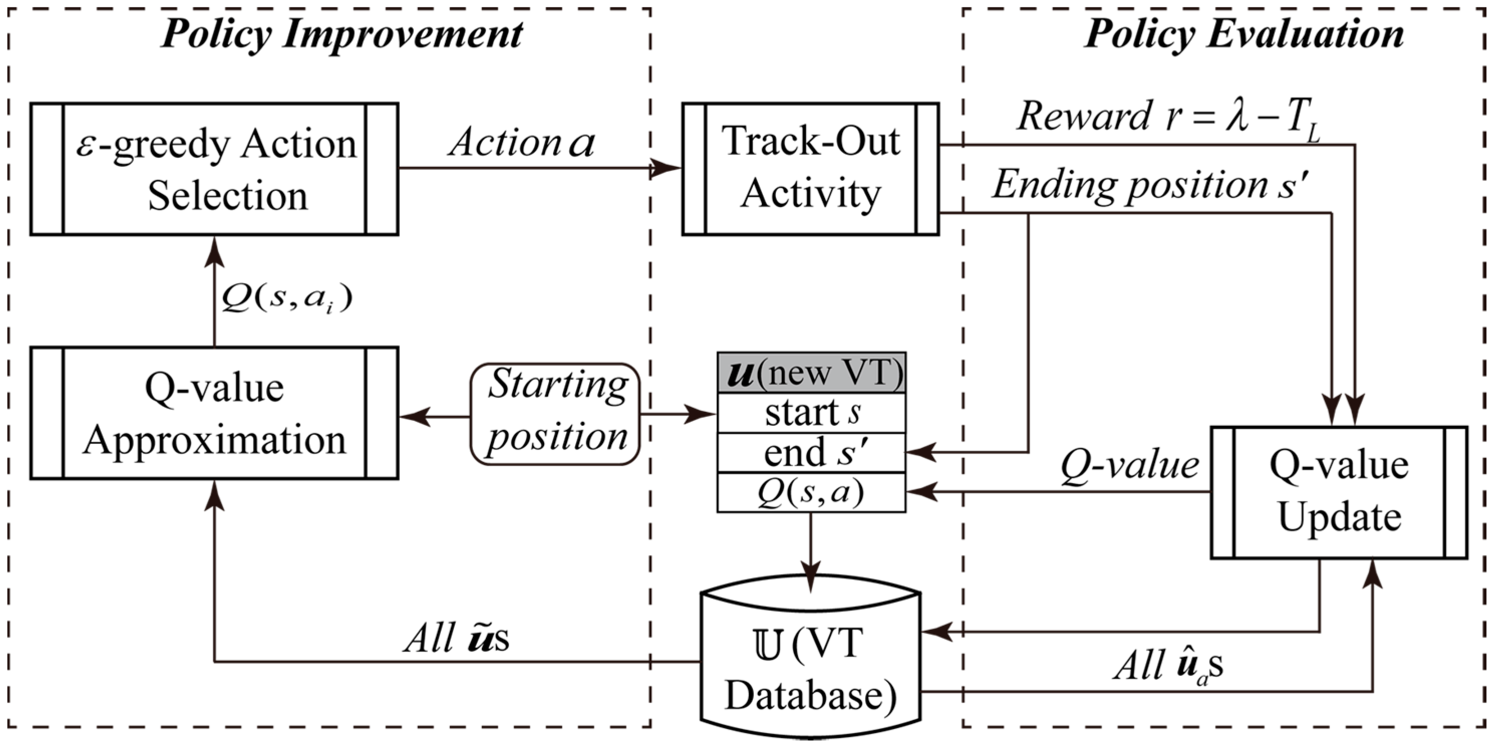
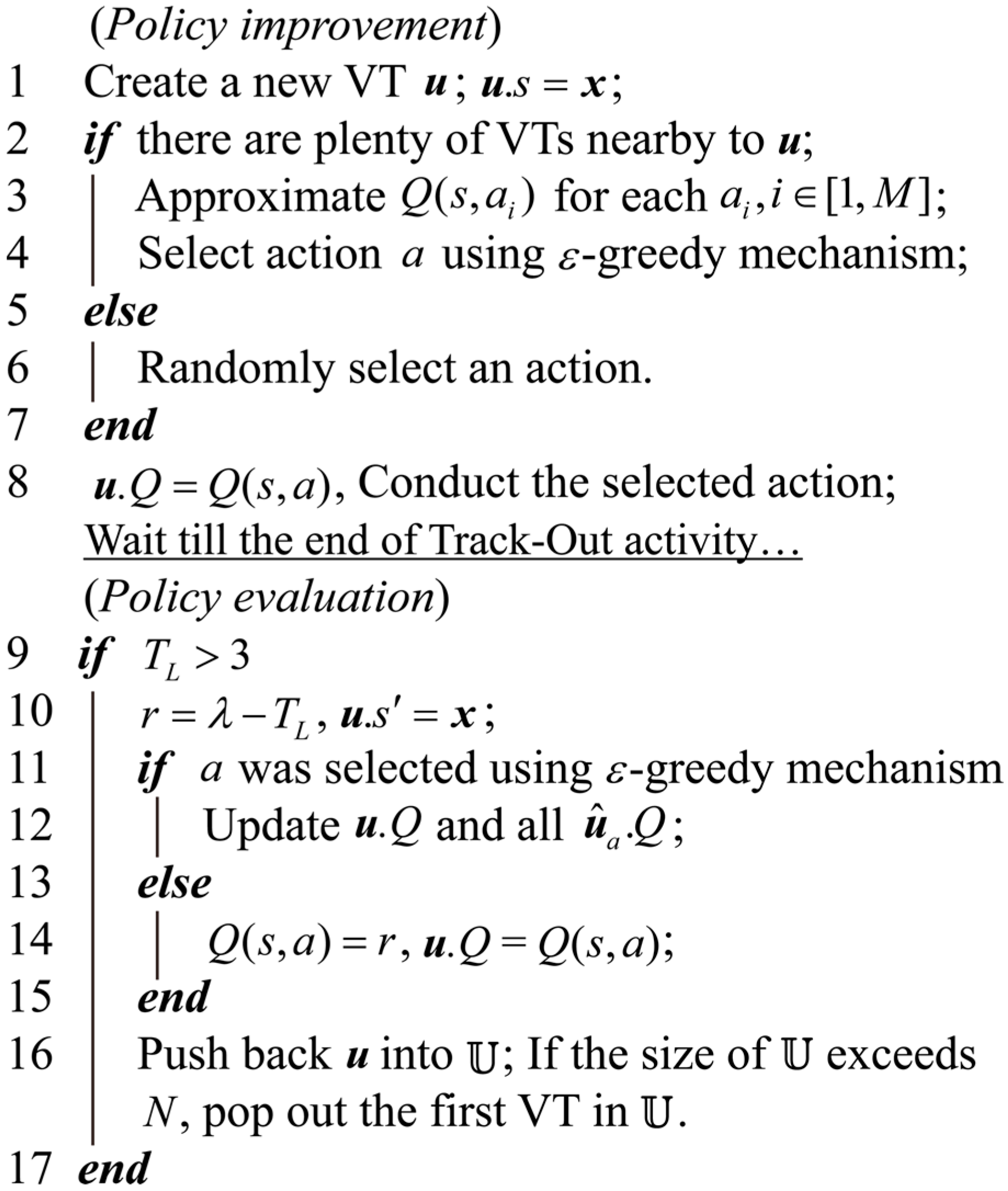
Policy Improvement

- (1)
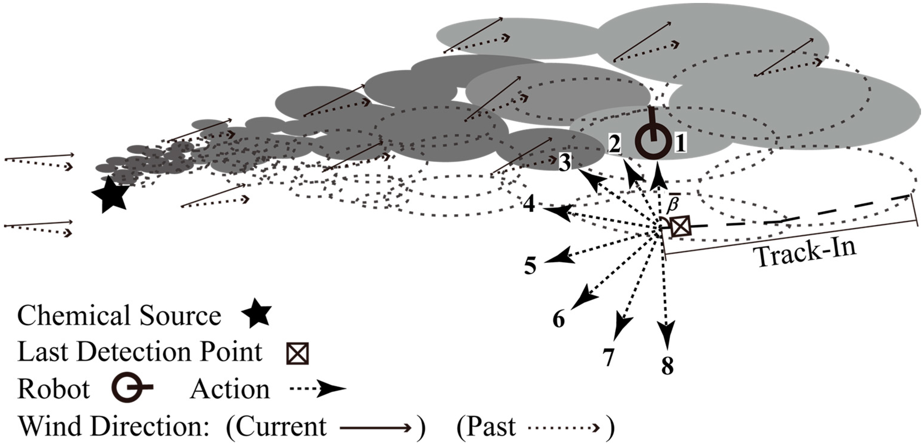
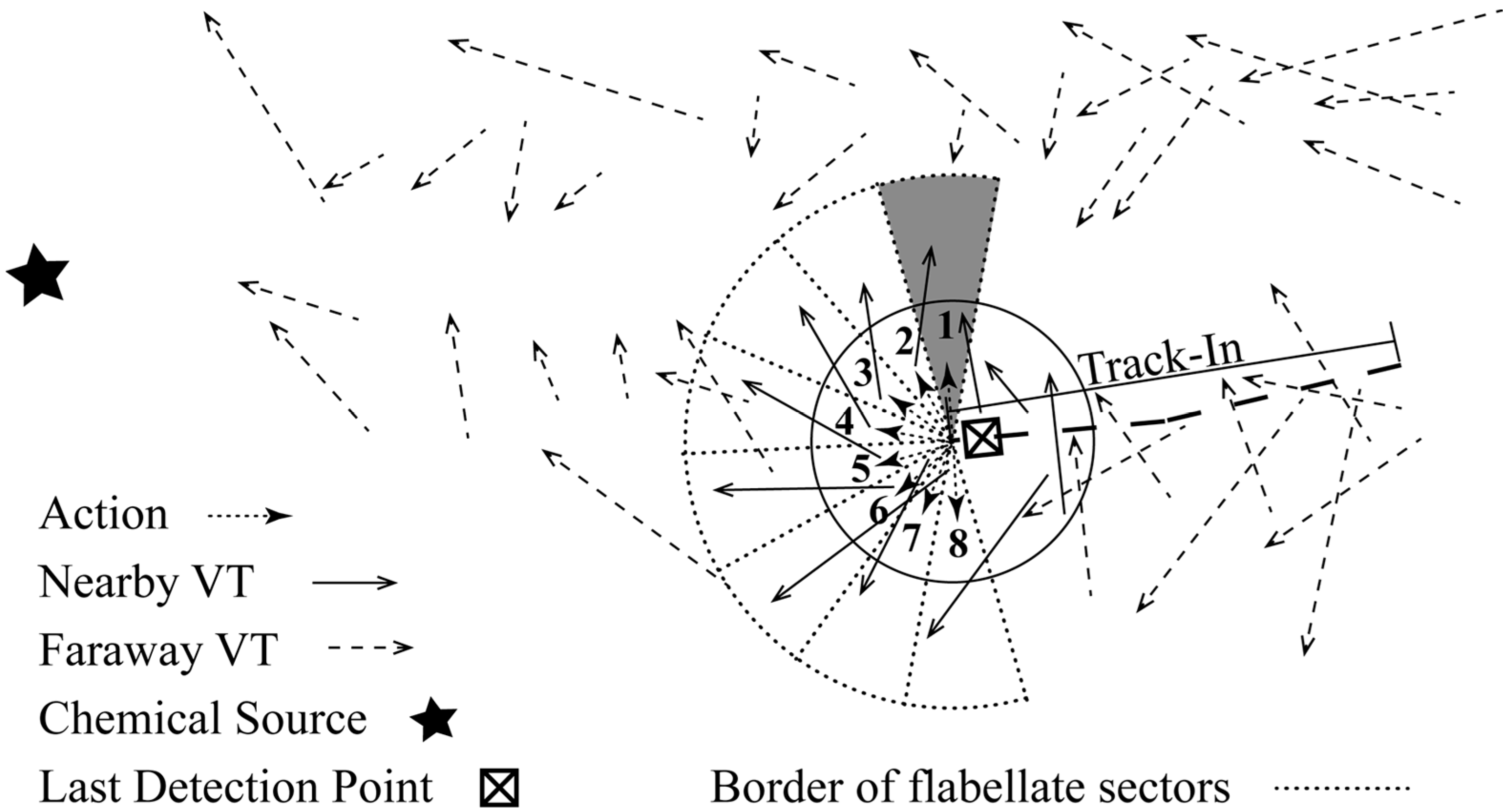
- Find nearby VTs of in the database, which are denoted as s. As mentioned, Q-value is approximated based on VTs that are previously stored in a VT database . In Figure 6, nearby and faraway VTs are represented as solid and dashed arrows, respectively.
- (2)
- Associate the nearby stored VTs with the actions. Suppose that covers a flabellate sector bi-partitioned by . In Figure 6, the flabellate sector covered by is marked as shadowed. The radius and included angle of the flabellate sector are ( is the maximal velocity of the robot) and , respectively. Then, if the end state of falls within the sector covered by , is associated with . The VT associated with is denoted as . In Figure 6, there are two VTs associated with , while there is only one VT associated with each of other actions.
- (3)
- Approximate by weighted-averaging the Q-value of all s. The weight for the Q-value of the j-th (i.e., ), which is denoted as , is calculated as:where and are the start state and the Q-value of , respectively; is the distance between and .
Policy Evaluation
3.2. Collaborative VTF Method
- (1)
- During policy improvement, the VTs in the same database are exploited by multiple robots in the LWA-based Q-value approximation. In other words, the robots determine their own heading by learning from the experience of each other at the beginning of Track-Out activities.
- (2)
- The Q-value of nearby VTs stored in the same database are updated by multiple robots. Moreover, the VTs generated by multiple robots are pushed into the same database after policy evaluation.
4. Experimental Setup
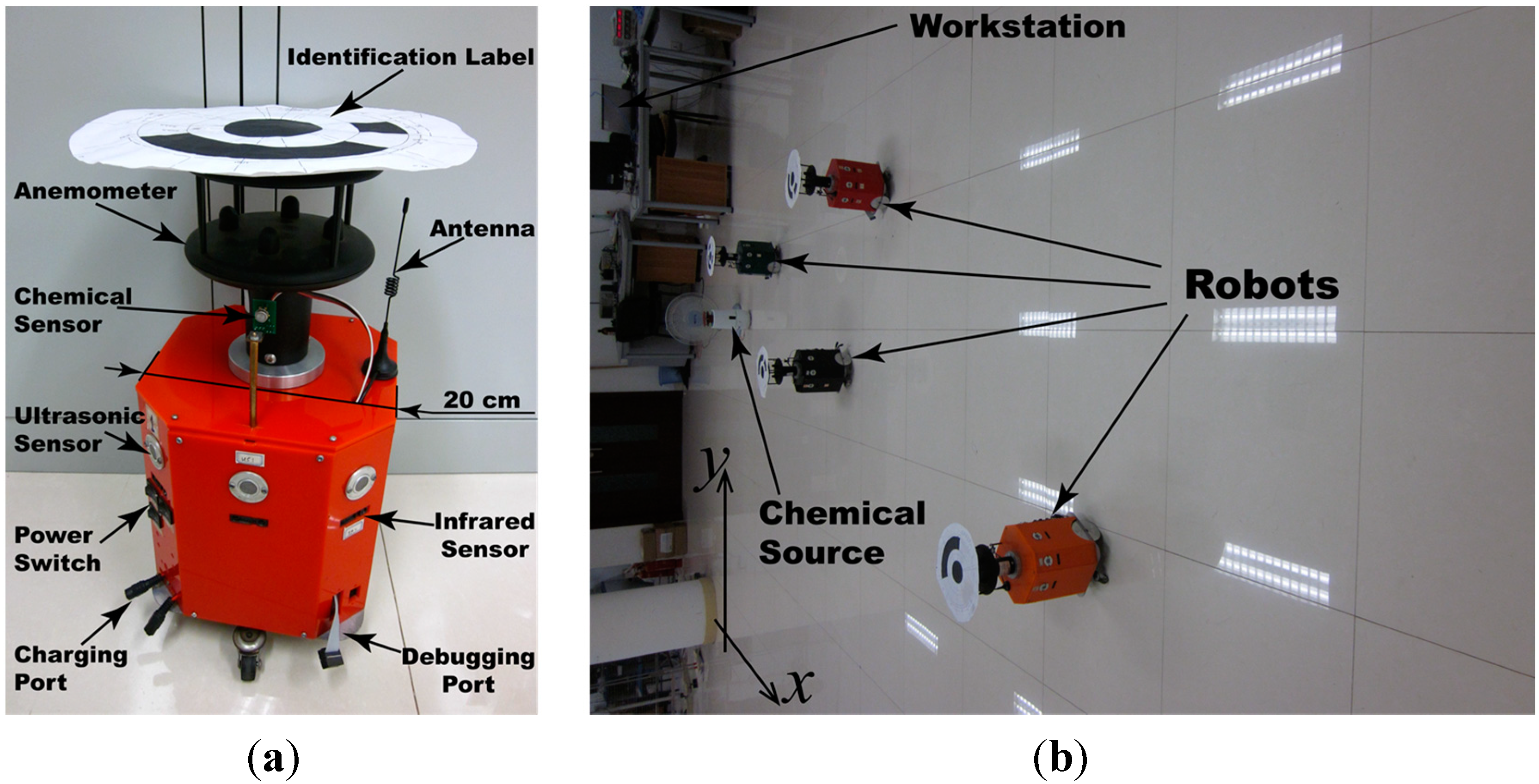
4.1. Real olfactory robots

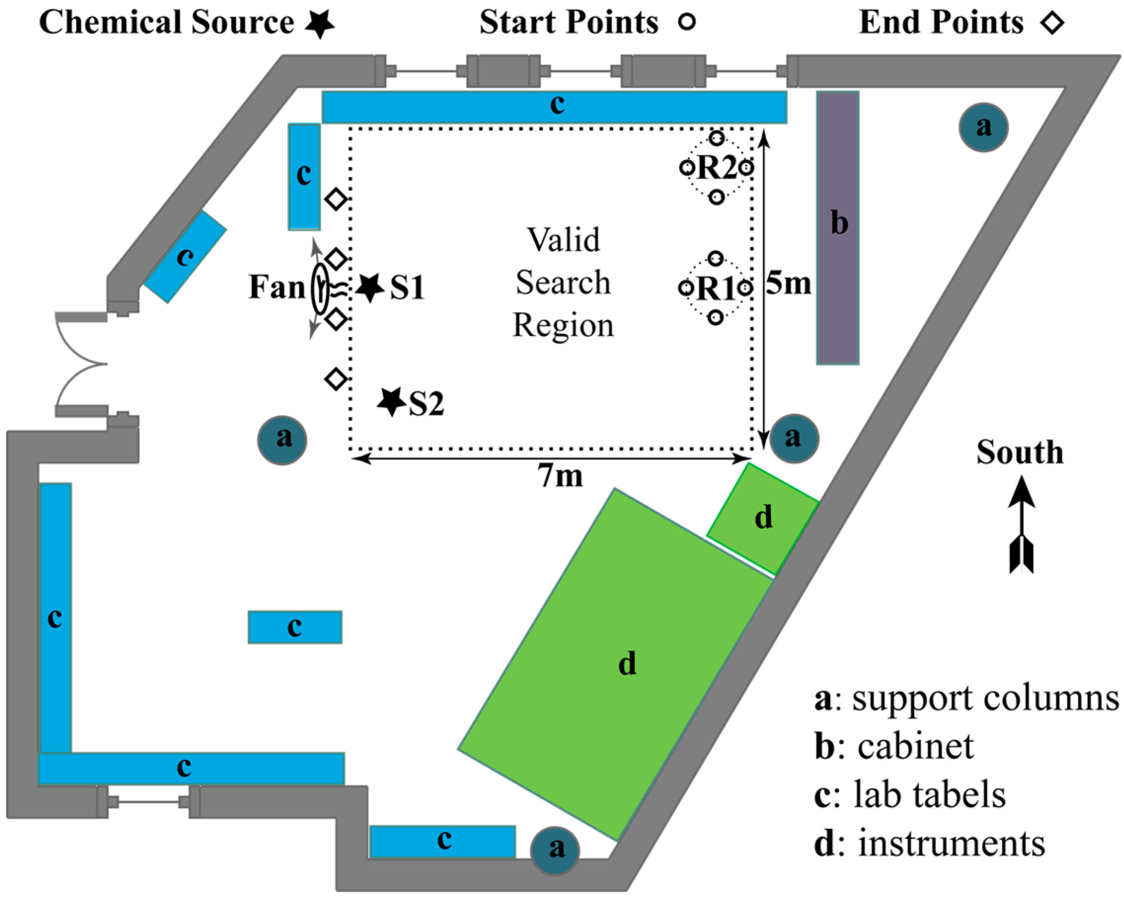
4.2. Experimental Scenarios
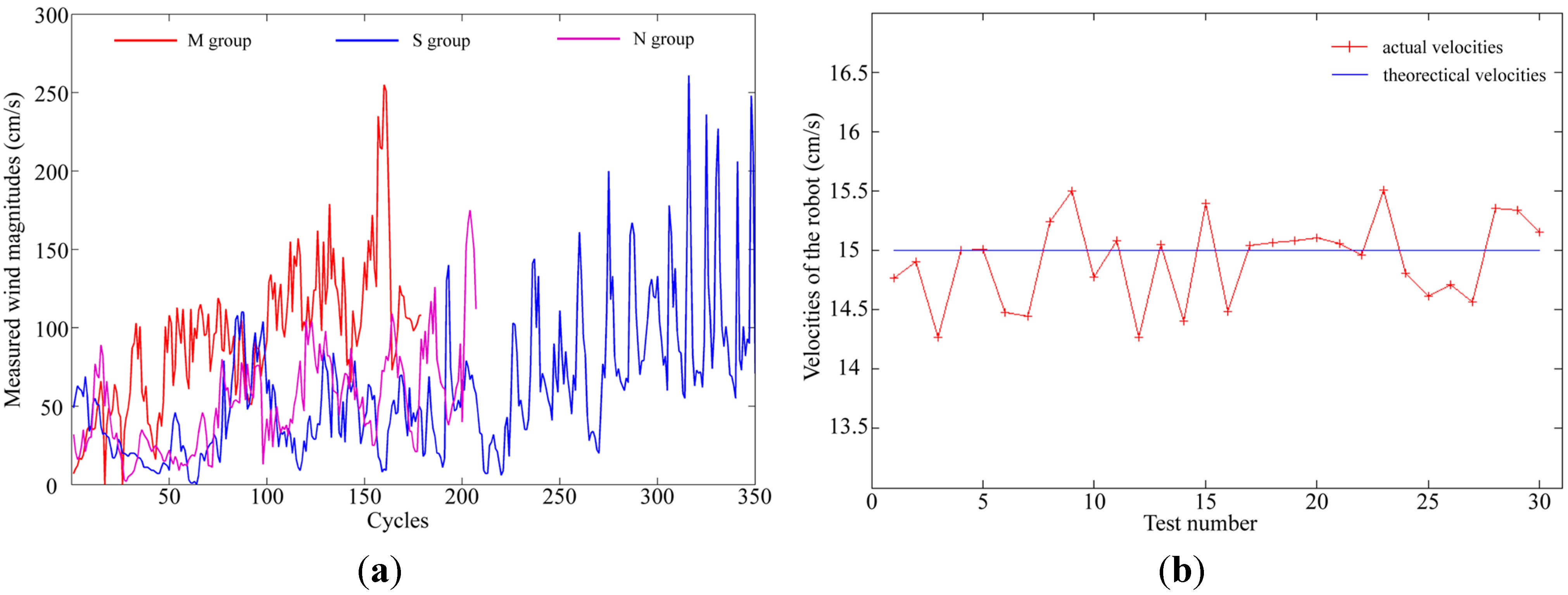
- Two controlled airflow fields: With the door and all windows of the laboratory closed, mildly and severely fluctuating wind were produced by oscillating the fan with scopes of about and , respectively. In these two controlled airflow fields, the chemical source was placed at S1, and the robots started from R1.
- Naturally ventilated airflow field was constructed by opening the windows and the door of the laboratory in a windy day. The chemical source was placed at S2, so that the released chemical can be blown by the wind coming from the door and the window in the bottom wall. The robots started from R2.

4.3. Experimental Scheme
- (1)
- Moving along a designed direction (e.g., upwind direction in Track-In activities, the direction learned in Track-Out activities): was set to a position in front of the robot along the designed direction. To move the robot at along direction , for example, the goal position was set to:where should be big enough to make sure the APF method outputs sufficient attractive force for the robot.
- (2)
- Cross-wind movement with gradually broadened scanning widths in the “casting” behaviour [13]: Suppose the robot position at the beginning of “casting” was . During the “casting” behavior, the robot was moved towards . Once the robot arrived at the old position of , was reset as follows:where , , and are the y-coordinate of , the number of times that the robot has arrived at , and the scanning span added to the scanning width, respectively. Note that the resulting robot trajectories do not strictly equal the one illustrated in [13] and [14]. Nevertheless, plume reacquiring behaviour is not the main concern of this paper.
4.4. Parameter Selection
- (1)
- (2)
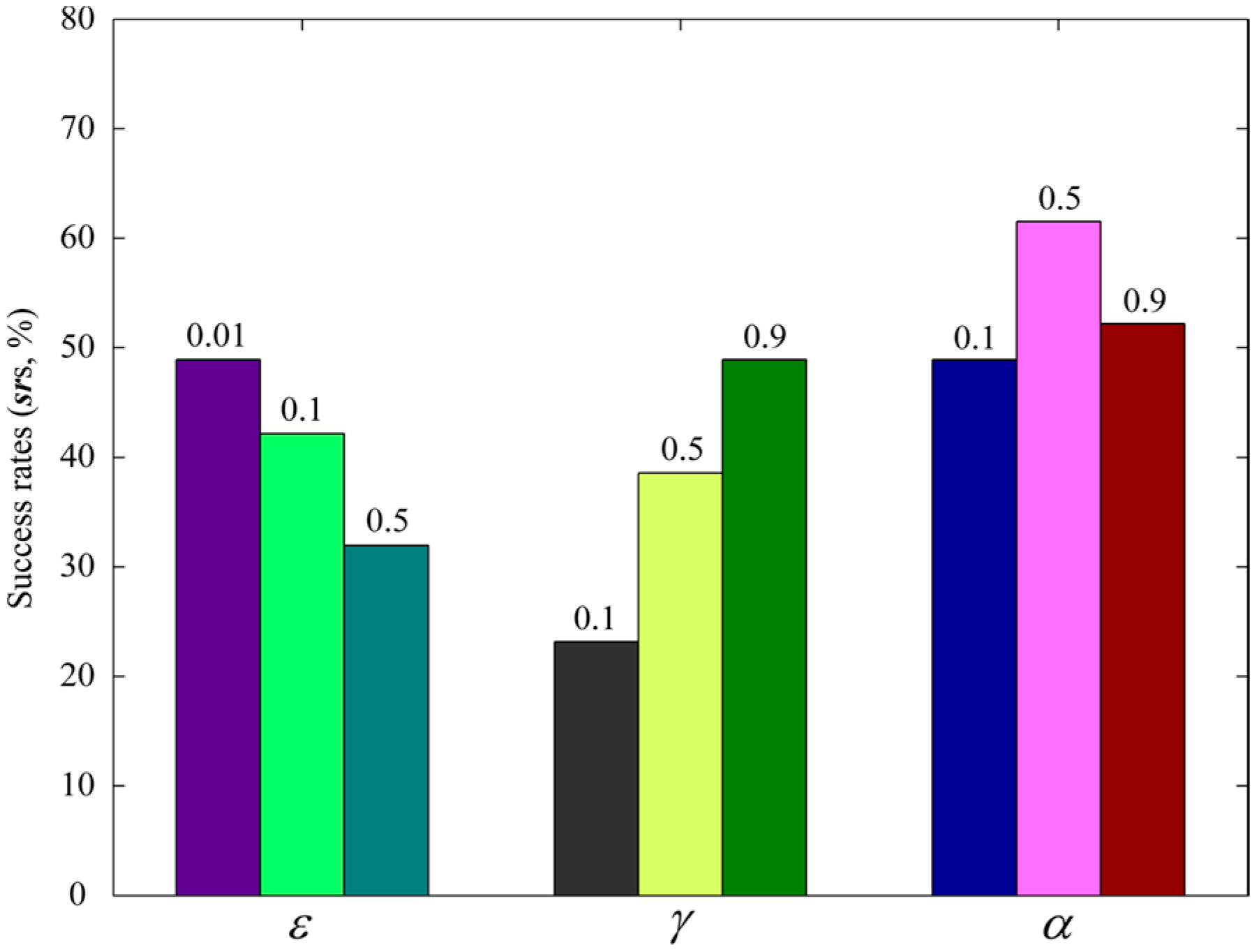
- Parameters for RL: , , and . In an analogous continuous instance-based Q learning method [25], , , and were set to 0.01, 0.9, and 0.1, respectively.
- (3)
- Parameters for obstacle avoidance using the APF method: , , , and , which were set to 15 cm/s, 45 cm, 4 m, and 80 cm, respectively. The guideline for selecting these parameters is that the robots would not collide with each other while searching in the valid search region.
4.4.1. Selecting the Common Parameters of Track-Out Activity

4.4.2. Selecting the Parameters for RL
5. Results and Discussion
5.1. Experimental Results
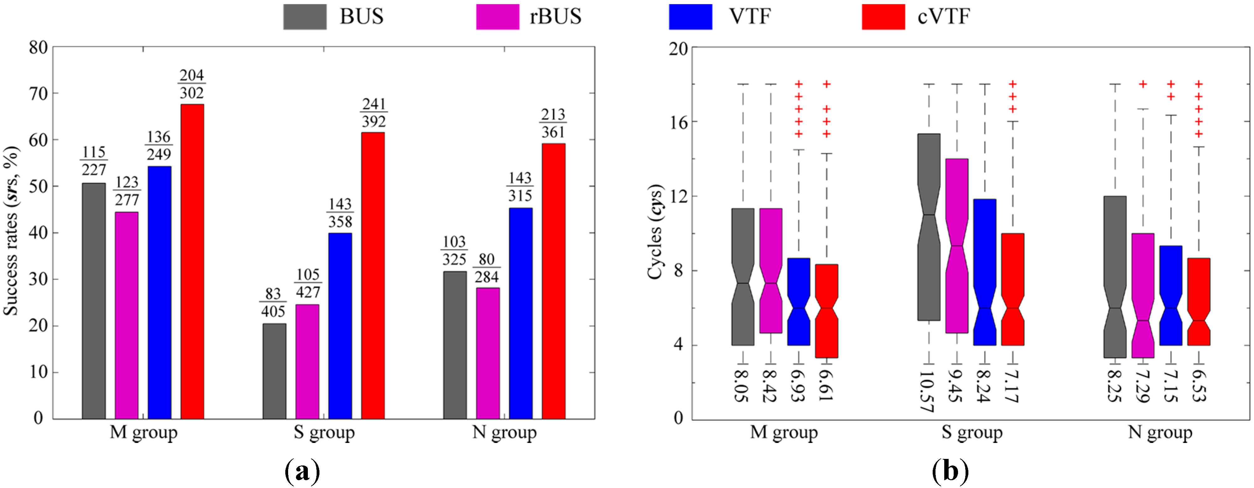
5.1.1. Success Rates

5.1.2. Time-Efficiency
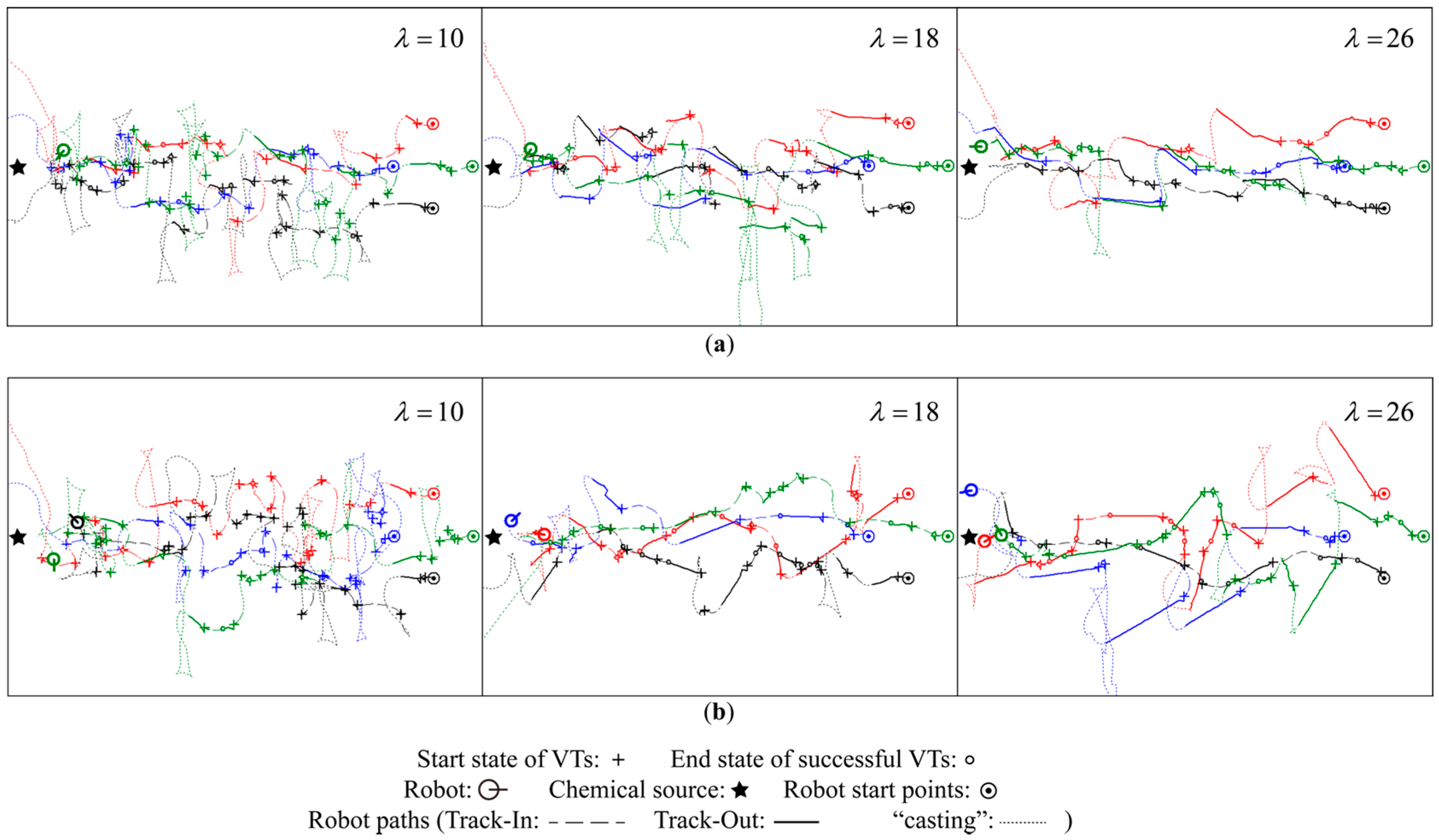
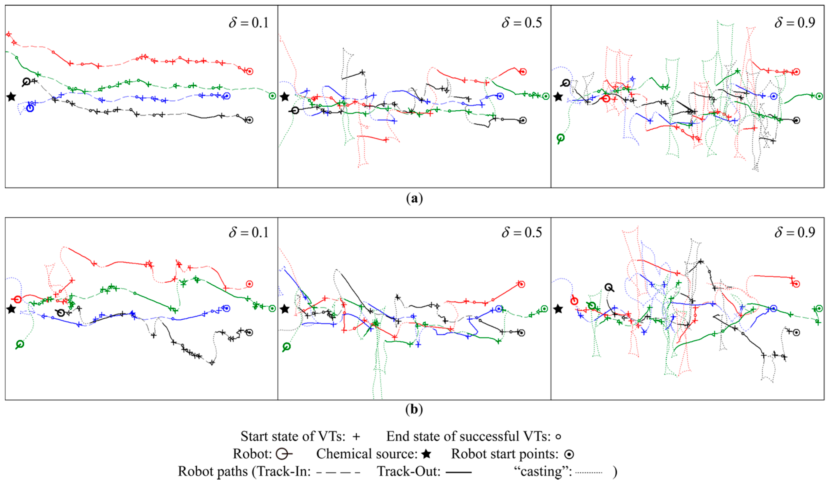
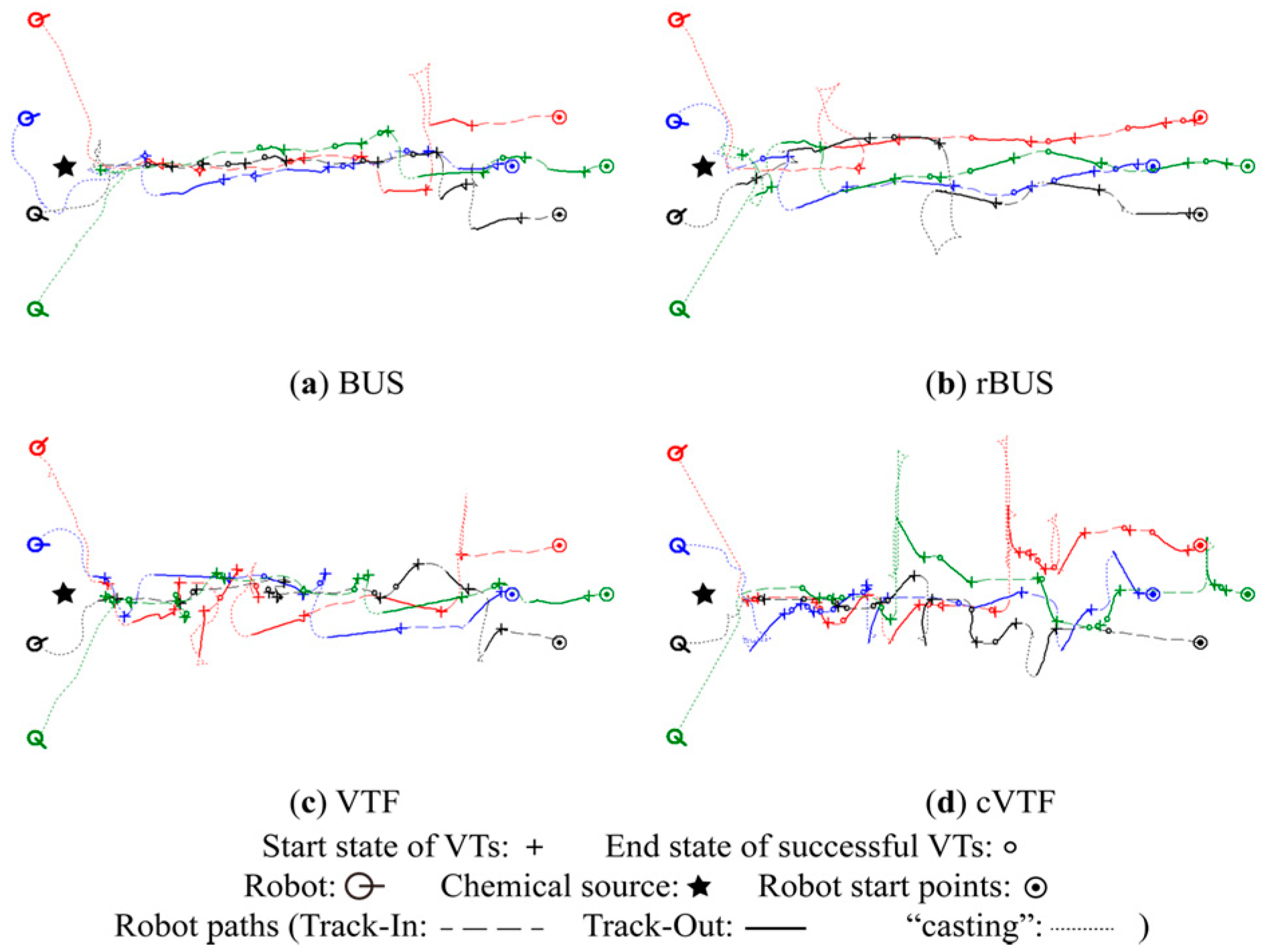
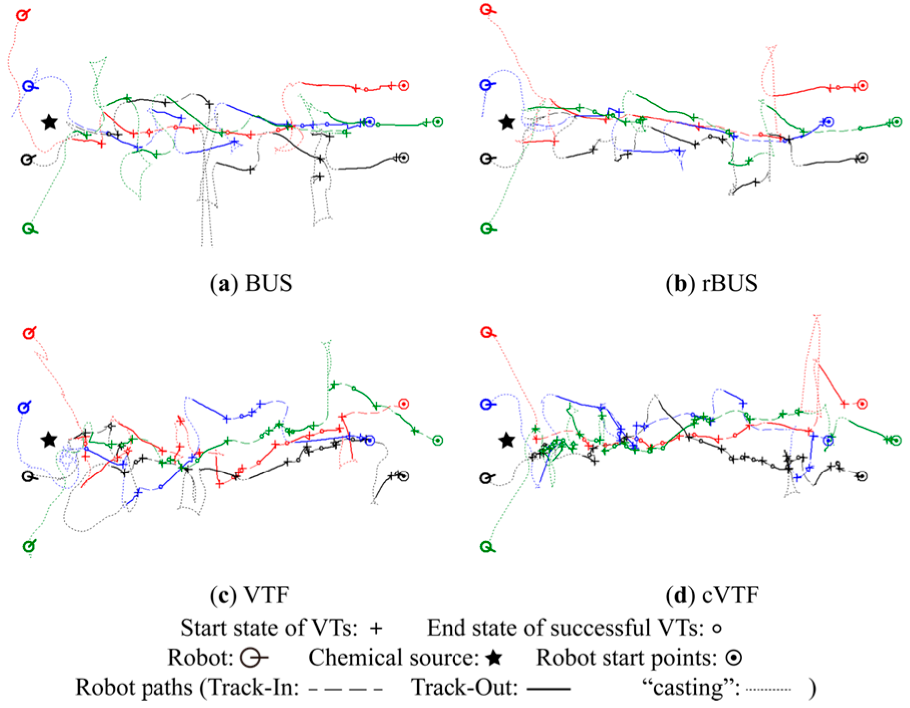
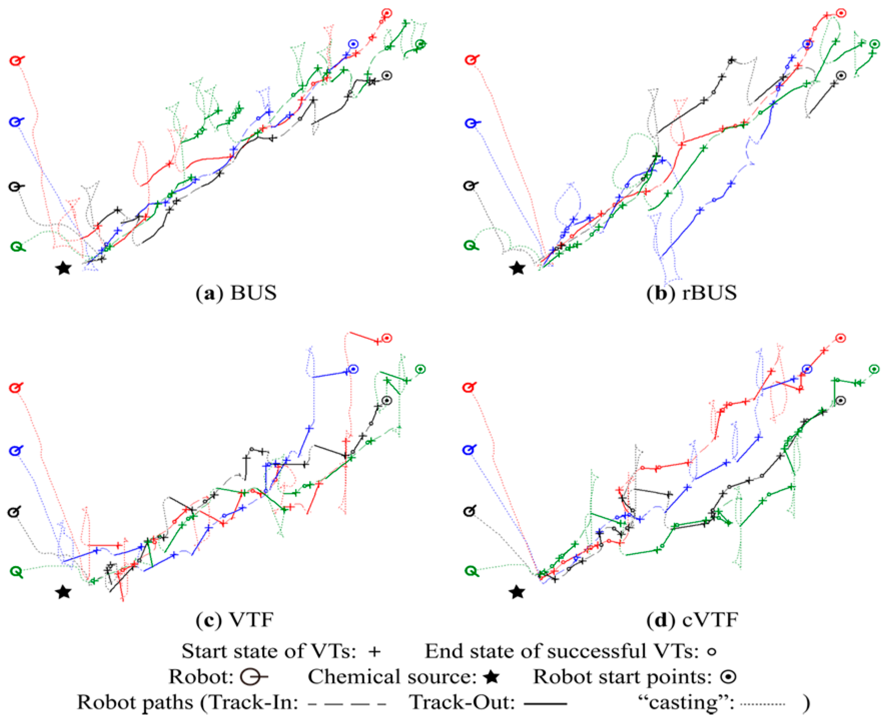
5.1.3. Robot Trajectories
Qualitative Analysis


Quantitative Analysis

| BUS | rBUS | VTF | cVTF | |
|---|---|---|---|---|
| M group | 1.0162 | 1.0178 | 1.2474 | 1.2647 |
| S group | 1.0116 | 1.0184 | 1.4782 | 1.5280 |
| N group | 1.0201 | 1.0193 | 1.6045 | 1.6893 |
5.2. Discussion
6. Conclusions

Acknowledgments
Author Contributions
Appendix
| Number of cycles from the last chemical detection event till the current time. | |
| Cycle limit for the Track-Out activity. | |
| Cycle limit for the plume re-acquiring behavior. | |
| Robot heading at the k-th cycle for BUS; Robot heading learned by VTF/cVTF. | |
| Bias angle at the k-th cycle for BUS; Bias angle learned by VTF/cVTF. | |
| Angle of wind direction measured at the k-th cycle and LDP, respectively. | |
| Position of the robot at the k-th cycle and LDP, respectively. | |
| State, action, and reward at the k-th cycle, respectively. | |
| Action value when action is conducted at state and thereby following policy . | |
| Learning rate used in VTF/cVTF. | |
| Discount rate used in VTF/cVTF. | |
| Probability of selecting random action in the -greedy selection mechanism. | |
| Number of actions. | |
| Start state, end state, and Q-value of the new VT , respectively. | |
| Nearby VT of . | |
| The VTs associated with action . | |
| Database for storing VTs. | |
| Size limit of .Size limit of . | |
| The weight for the j-th VT associated with action . | |
| Transient concentration measurement at the k-th cycle. | |
| Adaptive concentration threshold at the k-th cycle. | |
| Constant parameter for calculating . | |
| Goal position of the robot. | |
| Distance threshold for determining whether to generate repulsive force or not. | |
| A distance that is big enough for APF to generate sufficient attractive force. | |
| Number of times that the robot has arrived at in “casting” behavior. | |
| Scanning span added to the scanning width in “casting” behavior. | |
| The maximal velocity of the robot. |
Conflicts of Interest
References
- Quinn, T.P. The Behavior and Ecology of Pacific Salmon and Trout; University of Washington Press: Seattle, WA, USA, 2005. [Google Scholar]
- Lecchini, D.; Mills, S.C.; Brié, C.; Maurin, R.; Banaigs, B. Ecological determinants and sensory mechanisms in habitat selection of crustacean postlarvae. Behav. Ecol. 2010, 21, 599–607. [Google Scholar] [CrossRef]
- Weissburg, M.J.; Dusenbery, D.B. Behavioral observations and computer simulations of blue crab movement to a chemical source in a controlled turbulent flow. J. Exp. Biol. 2002, 205, 3387–3398. [Google Scholar] [PubMed]
- Pravin, S.; Reidenbach, M. Simultaneous sampling of flow and odorants by crustaceans can aid searches within a turbulent plume. Sensors 2013, 13, 16591–16610. [Google Scholar] [CrossRef] [PubMed]
- Cardé, R.; Willis, M. Navigational strategies used by insects to find distant, wind-borne sources of odor. J. Chem. Ecol. 2008, 34, 854–866. [Google Scholar] [CrossRef]
- Vergassola, M.; Villermaux, E.; Shraiman, B.I. “Infotaxis” as a strategy for searching without gradients. Nature 2007, 445, 406–409. [Google Scholar] [CrossRef] [PubMed]
- Cao, M.-L.; Meng, Q.-H.; Zeng, M.; Sun, B.; Li, W.; Ding, C.-J. Distributed least-squares estimation of a remote chemical source via convex combination in wireless sensor networks. Sensors 2014, 14, 11444–11466. [Google Scholar] [CrossRef] [PubMed]
- Ishida, H. Robotic systems for gas/odor source localization: Gap between experiments and real-life situations. In Proceedings of the IEEE International Conference on Robotics and Automation, Roma, Italy, 10–14 April 2007.
- Li, W.; Farrell, J.A.; Carde, R.T. Tracking of fluid-advected odor plumes: Strategies inspired by insect orientation to pheromone. Adapt. Behav. 2001, 9, 143–170. [Google Scholar] [CrossRef]
- Li, W.; Farrell, J.A.; Pang, S.; Arrieta, R.M. Moth-inspired chemical plume tracing on an autonomous underwater vehicle. IEEE Trans. Robot. 2006, 22, 292–307. [Google Scholar] [CrossRef]
- Marques, L.; Nunes, U.; de Almeida, A.T. Olfaction-based mobile robot navigation. Thin Solid Films 2002, 418, 51–58. [Google Scholar] [CrossRef]
- Lilienthal, A.J.; Reimann, D.; Zell, A. Gas source tracing with a mobile robot using an adapted moth strategy. In Autonome Mobile Systeme; Dillmann, R., Wörn, H., Gockel, T., Eds.; Springer: Berlin, Germany, 2003; pp. 150–160. [Google Scholar]
- Ishida, H. Odor-source localization by mobile robot and inter-robot communication using odors. In Olfactory Display: Multimedia Tool for Presenting Scents; Nakamoto, T., Ed.; Fragrance Journal Ltd.: Tokyo, Japan, 2008; pp. 191–198. [Google Scholar]
- Ishida, H.; Wada, Y.; Matsukura, H. Chemical sensing in robotic applications: A review. IEEE Sens. J. 2012, 12, 3163–3173. [Google Scholar] [CrossRef]
- Lilienthal, A.J.; Loutfi, A.; Duckett, T. Airborne chemical sensing review. Sensors 2006, 6, 1616–1678. [Google Scholar] [CrossRef] [Green Version]
- Neumann, P.P.; Asadi, S.; Lilienthal, A.J.; Bartholmai, M.; Schiller, J.H. Autonomous gas-sensitive microdrone: Wind vector estimation and gas distribution mapping. IEEE Robot. Autom. Mag. 2012, 19, 50–61. [Google Scholar] [CrossRef]
- Neumann, P.P.; Bennetts, V.H.; Lilienthal, A.J.; Bartholmai, M.; Schiller, J.H. Gas source localization with a micro-drone using bio-inspired and particle filter-based algorithms and particle filter-based algorithms. Adv. Robot. 2013, 27, 725–738. [Google Scholar] [CrossRef]
- Dunbabin, M.; Marques, L. Robots for environmental monitoring: Significant advancements and applications. IEEE Robot. Autom. Mag. 2012, 19, 24–39. [Google Scholar] [CrossRef]
- Sutton, R.S.; Barto, A.G. Reinforcement Learning: An Introduction; Cambridge University Press: Cambridge, UK, 1998; Volume 1. [Google Scholar]
- Larionova, S.; Almeida, N.; Marques, L.; de Almeida, A.T. Olfactory coordinated area coverage. Auton. Robot. 2006, 20, 251–260. [Google Scholar] [CrossRef]
- Gu, D.-B.; Yang, E.-F. Multiagent Reinforcement Learning for Multi-Robot Systems: A Survey; Teachnical Report CSM-404; University of Essex: Essex, UK, 2004. [Google Scholar]
- Watkins, C.J.; Dayan, P. Q-learning. Mach. Learn. 1992, 8, 279–292. [Google Scholar]
- Zhang, J.-W.; Rössler, B. Self-valuing learning and generalization with application in visually guided grasping of complex objects. Robot. Auton. Syst. 2004, 47, 117–127. [Google Scholar] [CrossRef]
- Atkeson, C.; Moore, A.; Schaal, S. Locally weighted learning. Artif. Intell. Rev. 1997, 11, 11–73. [Google Scholar] [CrossRef]
- Gu, D.-B.; Hu, H.-S. Teaching robots to plan through q-learning. Robotica 2005, 23, 139–147. [Google Scholar] [CrossRef]
- Meng, Q.-H.; Yang, W.-X.; Wang, Y.; Zeng, M. Collective odor source estimation and search in time-varient airflow environment. Sensors 2011, 11, 10415–10443. [Google Scholar] [CrossRef] [PubMed]
- Meng, Q.-H.; Yang, W.-X.; Wang, Y.; Zeng, M. Adapting ant colony metaphor for multi-robot chemical plume tracing. Sensors 2012, 12, 4737–4763. [Google Scholar] [CrossRef] [PubMed]
- Li, J.-G.; Meng, Q.-H.; Wang, Y.; Zeng, M. Odor source localization using a mobile robot in outdoor airflow environments with a particle filter algorithm. Auton. Robot. 2011, 30, 281–292. [Google Scholar] [CrossRef]
- Lilienthal, A.J. Gas Distribution Mapping and Gas Source Localization with a Mobile Robot. Ph.D. Thesis, University of Tubingen, Tubingen, Germany, 8 December 2004. [Google Scholar]
- Huang, L. Velocity planning for a mobile robot to track a moving target—A potential field approach. Robot. Auton. Syst. 2009, 57, 55–63. [Google Scholar] [CrossRef]
- Lochmatter, T. Bio-Inspired and Probabilistic Algorithms for Distributed Odor Source Localization Using Mobile Robots. Ph.D. Thesis, Swiss federal Institute of Technology in Lausanne, lausanne, Switzerland, 25 February 2010. [Google Scholar]
© 2015 by the authors; licensee MDPI, Basel, Switzerland. This article is an open access article distributed under the terms and conditions of the Creative Commons Attribution license (http://creativecommons.org/licenses/by/4.0/).
Share and Cite
Cao, M.-L.; Meng, Q.-H.; Wang, J.-Y.; Luo, B.; Jing, Y.-Q.; Ma, S.-G. Learning to Rapidly Re-Contact the Lost Plume in Chemical Plume Tracing. Sensors 2015, 15, 7512-7536. https://doi.org/10.3390/s150407512
Cao M-L, Meng Q-H, Wang J-Y, Luo B, Jing Y-Q, Ma S-G. Learning to Rapidly Re-Contact the Lost Plume in Chemical Plume Tracing. Sensors. 2015; 15(4):7512-7536. https://doi.org/10.3390/s150407512
Chicago/Turabian StyleCao, Meng-Li, Qing-Hao Meng, Jia-Ying Wang, Bing Luo, Ya-Qi Jing, and Shu-Gen Ma. 2015. "Learning to Rapidly Re-Contact the Lost Plume in Chemical Plume Tracing" Sensors 15, no. 4: 7512-7536. https://doi.org/10.3390/s150407512
APA StyleCao, M.-L., Meng, Q.-H., Wang, J.-Y., Luo, B., Jing, Y.-Q., & Ma, S.-G. (2015). Learning to Rapidly Re-Contact the Lost Plume in Chemical Plume Tracing. Sensors, 15(4), 7512-7536. https://doi.org/10.3390/s150407512