2. Preliminaries and Problem Formulation
2.1. IEEE 802.15.4 CSMA/CA Protocol
In this section, a brief overview of the IEEE 802.15.4 CSMA/CA protocol is first provided, focusing on the details that are related to the proposed study. A more comprehensive introduction can be found in [
27].
The 802.15.4 is part of the IEEE family of standards that defines the physical layer (PHY) and medium access layer (MAC) for wireless personal area networks (WPAN). It is intended for devices with low power data rate, low complexity and stringent power requirement. The raw data rate in industrial, scientific and medical (ISM) band is 250 kbps. The basic time unit “slot” is defined as the unit backoff period which contains 10 bytes. In the time-slotted beacon-enabled mode, a superframe structure is used to govern the packet transmission. Each superframe begins with a beacon sent by the coordinator, followed by an active portion and an optional inactive portion. The active portion consists of a contention-access part and an optional contention-free part.
This paper considers the slotted CSMA/CA in the contention access portion. In a slotted CSMA/CA network, a node trying to transmit a packet would first initialize the counter called the number of backoffs (NB). Then the node performs the backoff algorithm to delay for a random number of time slots which is uniformly distributed in the range of , where BE is the backoff exponent. When the backoff period is over, the node performs a clear channel assessment (CCA) to detect whether the channel is idle. The node would begin to transmit data if two consecutive CCAs are idle. Otherwise, the node would increase the number of NB and BE by one, without exceeding the maximum backoff limit m and maximum backoff exponent respectively. The packet will be discarded if NB exceeds m. Otherwise, the node will start to transmit a packet after performing two CCAs to confirm that the channel is idle. An ACK would indicate successful transmission. If the node fails to receive ACK due to collision or ACK timeout, the packet will be considered a failure assuming that no retransmission mechanism is implemented.
2.2. Problem Formulation
Consider a generic single-hop network where
N nodes contend to transmit packets to a central node (
i.e., the coordinator) using the IEEE 802.15.4 slotted CSMA/CA protocol. Each node
is assigned a throughput demand of
. For convenience,
is defined as the ratio of the number of successful packets to the number of time slots during a certain time period,
i.e., on average node
i needs to successfully transmit a packet every
slots. Due to the backoff failure and packet collision, packet transmissions may fail and the packet success rate of node
is smaller than 1. It is assumed in this paper that packet loss due to MAC layer contention dominates other forms of packet loss such as path loss and channel fading. This assumption is reasonable as for most applications that operate in close proximity, packet loss on physical layer is usually negligible [
11,
28].
Assume node
has a transmission rate of
(e.g.,
means node
on average initialize a new packet transmission every 100 slots) and assume that
can be arbitrary tuned to meet the throughput demand. This feature applies to a wide variety of wireless industrial network systems [
29,
30,
31]. For example, for network control systems employing data rate theorem [
32], the transmission rate needs to be tuned frequently according to the channel condition to stabilize the control system. Another example would be a model-based network control system [
31], where the sensor packet generation needs to be tuned according to the dynamics of the control system.
can also be viewed as a probability that node
initializes a new packet transmission in a random time slot. Further assume that each packet lasts for
L slots and no retransmission is implemented on MAC layer (retransmission can be implemented on higher layer though). The objective of the proposed algorithm is for each node to find a suitable transmission rate
in a distributed manner such that:
Denote the vector the optimal operating point where every node meets its throughput demand. It is assumed in this paper that such a point always exists, i.e., the throughput demand is feasible. This assumption is reasonable in most sensor networks performing monitoring and control tasks as the data traffics generated by these nodes are usually below the capacity of the network.
In order to model the interactions in the network, it is essential to characterize the relationship between the two parameters of node
i, namely the probability that node
starts to perform CCA in a random time slot
and the probability that the CCA result is busy, namely busy channel probability
. Higher
indicates that a node will on average perform more backoffs for a certain packet and thus higher
, and
vice versa. This relationship can be quantified by calculating the average number of CCAs that node
experiences for each packet as follows:
where
enumerates all the possible number of CCAs and their corresponding probability. Furthermore,
also depends on every other node’s probability of starting to perform CCA in a random time slot
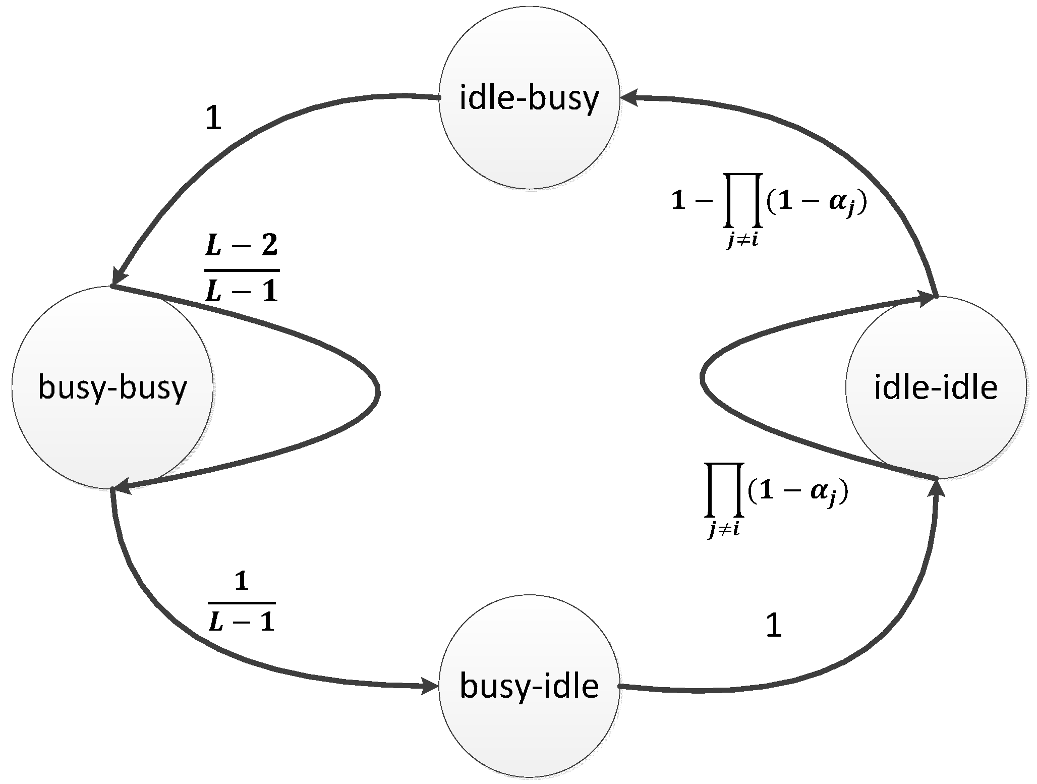
. This relationship can be characterized by the channel state model in
Figure 1 [
5].
Figure 1.
Channel state model.
Figure 1.
Channel state model.
The idea of the channel state model lies in the property of the CSMA/CA that a node needs to sense two successive idle slots before transmitting a packet. The channel state model is thus constructed to figure out what is the probability that a random adjacent slot-pair is idle. As such, the slotted channel is modeled as a discrete Markov chain whose states, namely idle-idle, idle-busy, busy-idle, busy-busy, are on an adjacent slot-pair basis [
5].
Each node has a unique channel state model, which reflects the traffics of all other nodes. Its state evolves as follows. If none of other nodes perform any transmissions, the channel state will be idle-idle. This happens with the probability . Otherwise, when at least one of the other nodes starts transmitting, the state goes to idle-busy and subsequently busy-busy. The state evolves to busy-idle once a packet transmission is completed, which happens with probability . Otherwise, the state stays at busy-busy. Finally, once the state changes to busy-idle, it will go to idle-idle with probability 1.
From the state evolution, the stationary channel state can be solved as , and , where , , and are the probabilities of node i that the slot-pair state is in idle-idle, busy-busy, idle-busy and busy-idle respectively, where .
The channel is considered busy when the slot-pair state is not
. Therefore,
can be determined as:
The difference from the work in [
5] is that instead of viewing the channel state as a whole, we model the channel from the perspective of an arbitrary node
. Each node has a unique channel state model. This slight yet important modification allows us to characterize the channel states in a distributed manner.
3. Distributed Transmission Rate Adjustment
Initially an arbitrary node
i, with no prior information, tentatively transmits data at the rate
. After a certain amount of time, node
i can estimate the busy channel probability
by recording the CCA information. The estimation is performed by calculating the ratio of the number of busy CCAs to the number of all the CCA for a certain period and using this ratio as the busy channel probability
.
is then used to determine the optimal
[
6,
8]. From Equation (3), once
is known,
can be determined as:
The term
contains transmission rate information of all other nodes
and can be rewritten using Equation (2) as:
One important observation is that for any 2 arbitrary node
and
, the backoff failure probability
and
are almost equal as long as the network size is not too small, or when the nodes are of homogeneous nature. This is because
and
are determined by
and
respectively and the ratio
is very close to 1 as
and
are typically smaller than 0.01 [
29,
33]. Thus the subscript
i for every
can be dropped without affecting the analysis. Combining Equations (4) and (5), one can get:
Our interest lies in finding a detailed characterization of the aggregate transmission rate
for
. However, it cannot be directly derived from Equation (6). Notice that in Equation (6), every
is sufficiently small (typically far smaller than 0.01 for non-saturated applications [
29,
33]) and when expanding the polynomial
, the second and higher order terms can be neglected without compromising the accuracy (e.g., the error when
and
N = 10 is less than 0.005). As such, Equation (6) can be rewritten in order to “isolate”
from other variables as follows:
From Equation (7),
can be given as:
From Equation (8), the aggregate transmission rate is explicitly related to the busy channel probability. Once
is determined, estimation of the busy channel probability at the optimal operating point can be performed. In the following analysis, the superscript
is used to denote variables at the optimal operating point. The optimal transmission rate for node
can be expressed as
, where
is ratio of the optimal transmission rate
to
. According to the channel state model, when the transmission rate of node
is
, the busy channel probability and the transmission rates of node
for
can be related as follows:
Using the same approximation technique as in Equation (7), Equation (9) can be rewritten as:
Solving Equation (10) for
yields:
In the meantime,
should satisfy
according to Equation (1). The packet success rate
of node
i can be expressed as follows [
34]:
where
is the probability that node
has access to an idle channel for a certain packet and
is the probability that at the same time there is no other node attempting to access the channel. Combining Equations (1), (7) and (12), one can obtain:
The objective here is to estimate
from
. As such, one can substitute Equations (11)–(13) to eliminate
as follows:
From Equation (14), it can be shown that is monotonically increasing in when by differentiating . Thus, an inverse function exists in this region.
In conclusion, given the values of , and , a unique can be readily solved and so is (using Equation (11)). Node can then use to determine its optimal transmission rate with respect to its throughput demand. In the actual implementation, the function can be discretized and computed using numerical methods and stored in a look-up table beforehand to simplify the computation.
5. Experimental Results
The proposed distributed algorithm has been implemented and extensively tested using the TelosB node [
36]. TelosB consists of a Texas Instrument MSP430F1611 microcontroller and an IEEE 802.15.4-complaint CC2420 radio transceiver. The proposed algorithm is built on top of the TinyOS operating system [
37], using a dialect of C language called nesC (network embedded system C language) [
38]. The codes for the proposed algorithm occupy about 8-kB program memory. For the medium access control (MAC) layer and the interfaces to the radio stack, the IEEE 802.15.4 slotted CSMA/CA implementation [
39] is used. The network is organized using star topology where multiple nodes transmit data to a pre-defined receiver. A packet transmission cycle consisting of transmitting the data packet and waiting and receiving the ACK packet is of 100 symbols long, which is translated to five time slots in the model in
Section 2. The function value
is discretized for
with an interval of 0.0025 using a “float” type C array as a look-up table.
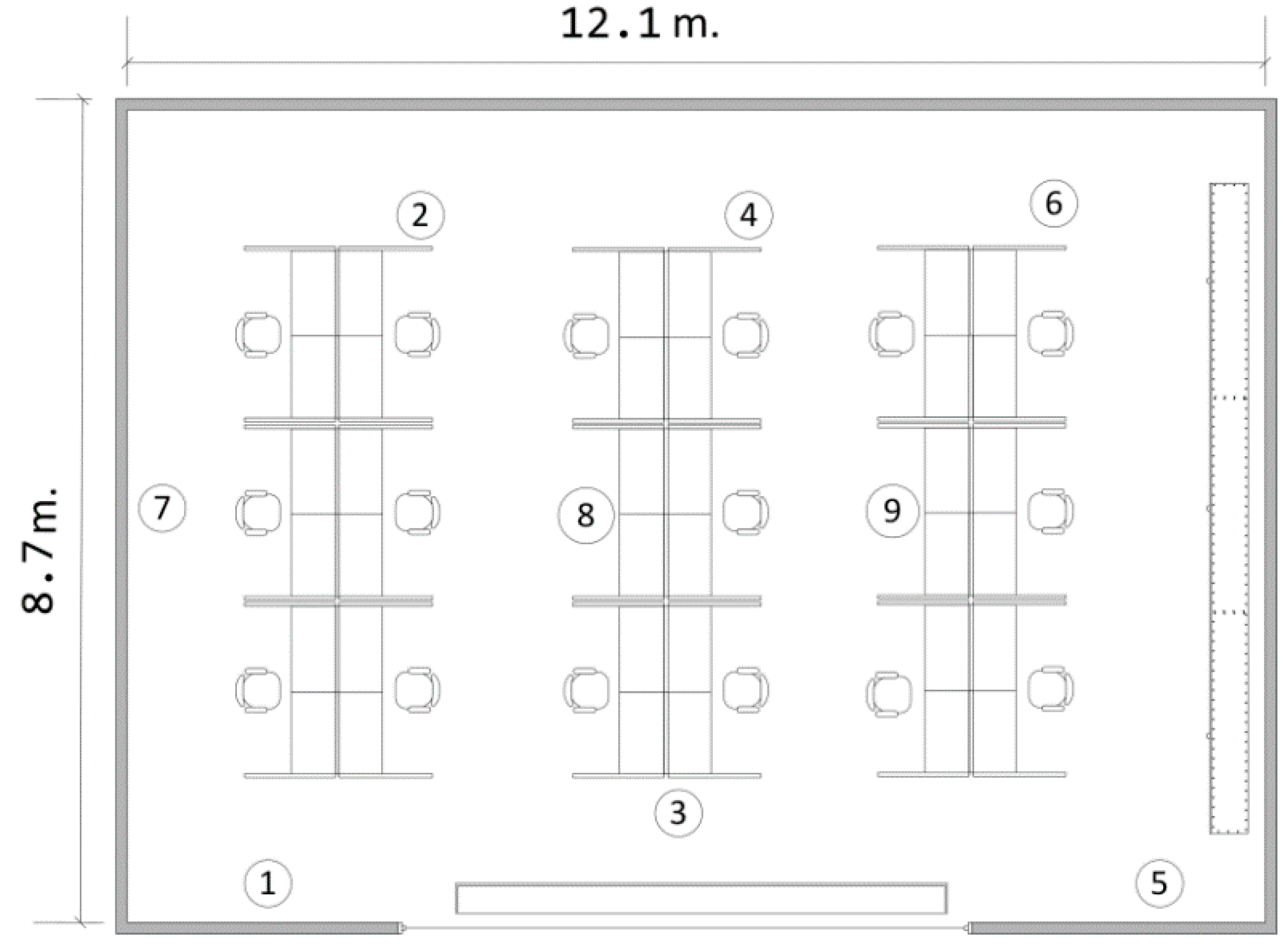
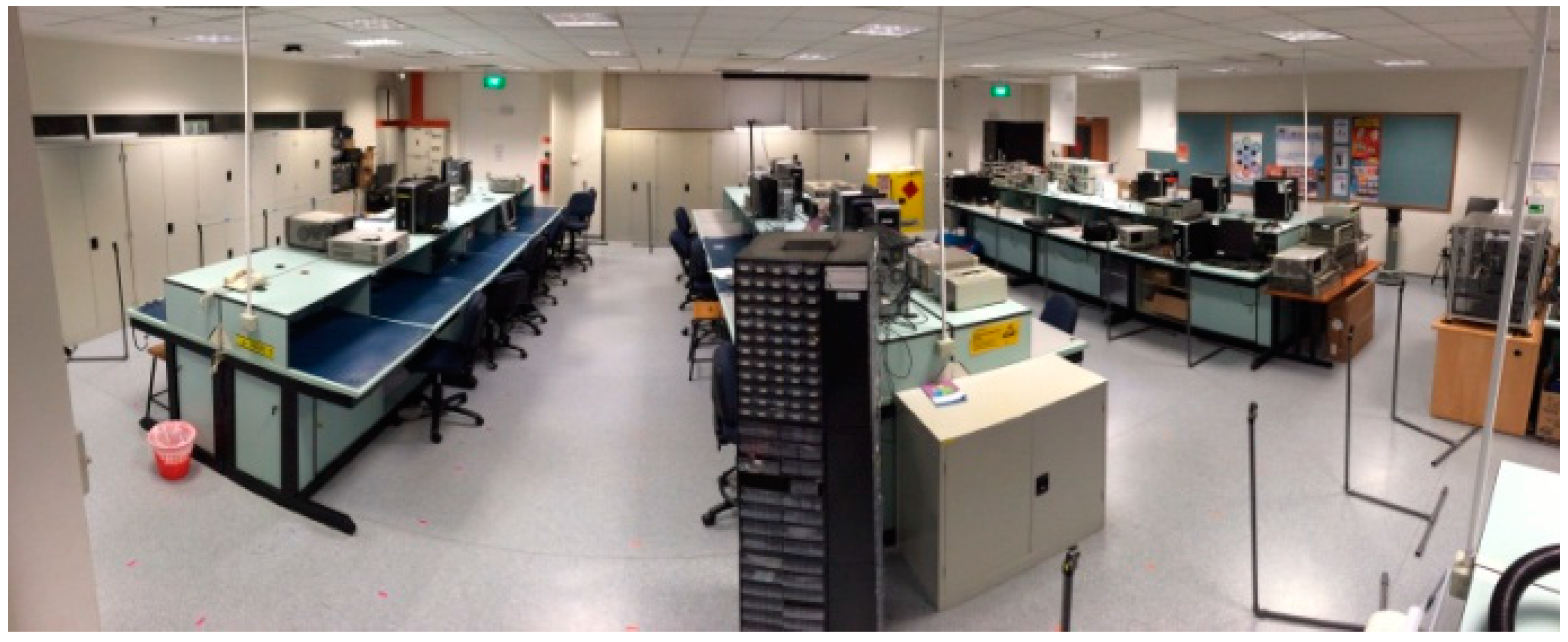
In the following discussions, the performance of the algorithm is evaluated under a typical laboratory environment, as shown in
Figure 4 and
Figure 5. Each node is placed on top of a 1-m PVC stand. The network to be tested is assumed to be a sparse and low-traffic network. The transmission power is set to 0 dBm. The application considered is an indoor laboratory monitoring and control system, where sensors of heterogeneous nature transmit packets to a central coordinator (controller). The traffic in such a system is unsaturated, but within a certain time interval, a minimum number of successful packets are expected (as “throughput demand”) for each sensor node in order to stabilize a control system, as discussed in [
30,
40], or to enable real-time monitoring. To take into account the effect of multi-path fading, the sensor nodes and the central coordinator are randomly placed in the nine spots in
Figure 5 and are shuffled after each experiment.
Figure 4.
The testing area.
Figure 4.
The testing area.
Figure 5.
The floor plan of the testing area.
Figure 5.
The floor plan of the testing area.
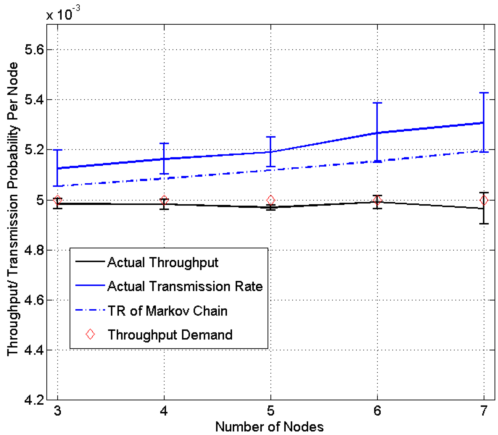
The homogeneous case where each sensor node in the network has the same throughput demand is first tested. Different numbers of sensor nodes in the network are evaluated, ranging from three to seven. Each node is assigned a throughput demand of 1/200. Each experiment is run for 300 s and repeated 3 times and more than 5000 packets are transmitted by each node for each experiment.
The result is shown in
Figure 6.
Figure 6 first compares the actual throughput (mean and standard deviation)
versus the throughput demand. It is observed that the actual throughput is very close to the demand, with an average relative error of 0.43%. The transmission rate (mean and standard deviation) is also compared with the one predicted using the Markov chain model [
5]. The result is in general very close but the proposed distributed algorithm performs slightly better in providing the optimal transmission rate based on the actual throughput.
Figure 6.
Experiment results of homogeneous networks (TR: transmission rate).
Figure 6.
Experiment results of homogeneous networks (TR: transmission rate).
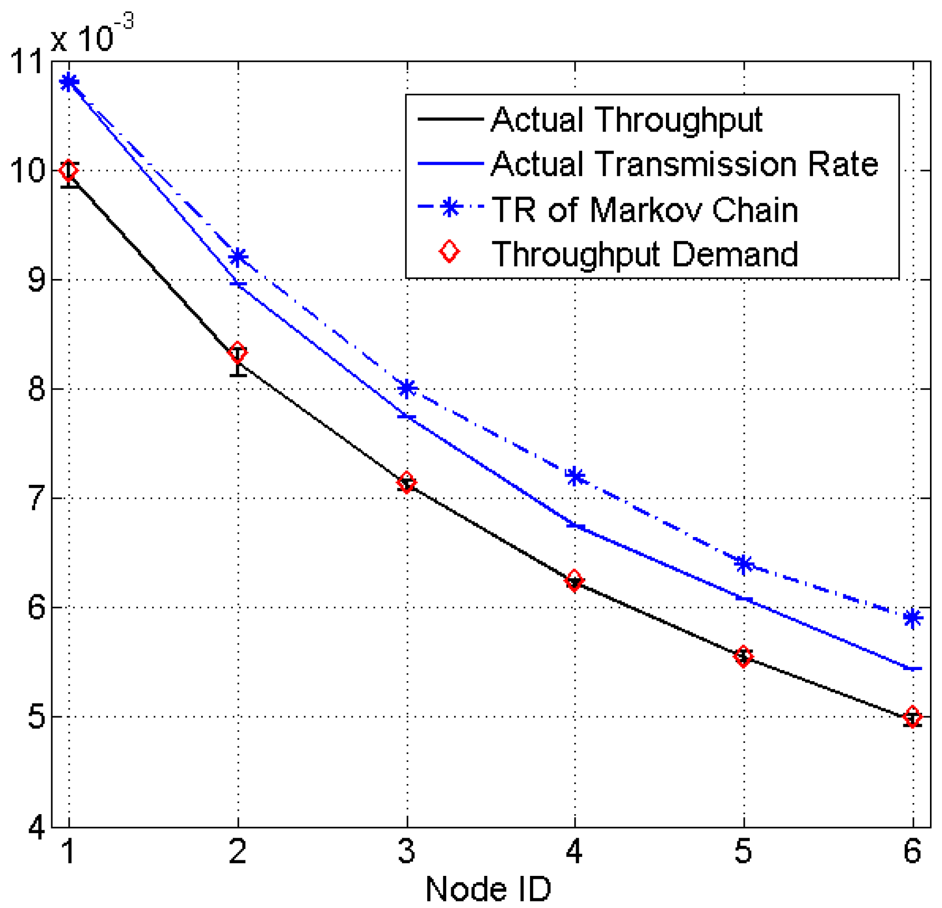
Figure 7 presents the result for a heterogeneous network consisting of six sensor nodes which are assigned a throughput demand of 1/100, 1/120, 1/140, 1/160, 1/180, 1/200, respectively. The experiment is run for 300 s and repeated 10 times. The actual throughput for each node matches very well with the demands, with an average percentage error of 0.524%.
Figure 7.
Experiment results of heterogeneous networks (TR: transmission rate).
Figure 7.
Experiment results of heterogeneous networks (TR: transmission rate).
Table 1 compares the proposed method with the Markov chain-based methods. It is shown that the proposed one is able to satisfy the throughput demand with a smaller error than the one achieved by the Markov chain model in both homogeneous networks and heterogeneous networks. This may be because the Markov chain model relies on certain assumptions (e.g., busy channel probability does not depend on backoff stages), which is prone to slight estimation errors. On the other hand, while the proposed algorithm also makes use of such models, the real-time CCA feedbacks can help to correct the modeling error and lead to a more accurate operating point with respect to the throughput demand. Moreover, due to its distributed nature, the proposed algorithm is easier to implement and requires local channel sensing information only while the Markov chain method is more computationally expensive and requires certain network-wide information. Lastly, the proposed method employs a real-time traffic estimation method and is able to adapt to possible traffic changes while in the case of the Markov chain method, a new model will need to be solved when there is a traffic change.
Table 1.
Comparisons of the proposed method and the Markov-chain based Methods.
Table 1.
Comparisons of the proposed method and the Markov-chain based Methods.
| Method | Proposed Method | Markov Chain-Based Methods |
|---|
| Errors | Homogeneous | 0.43% | 3.2% |
| Heterogeneous | 0.524% | 4.7% |
| Complexity | easy to implement; able to be stored in a look-up table | computationally intensive; requires solving of multi-dimension Markov chain |
| Required Information | local information only, e.g., channel sensing result | needs network-wide information, e.g., the number of active nodes |
| Flexibility | able to adapt traffic changes | requires the traffics to be constant |
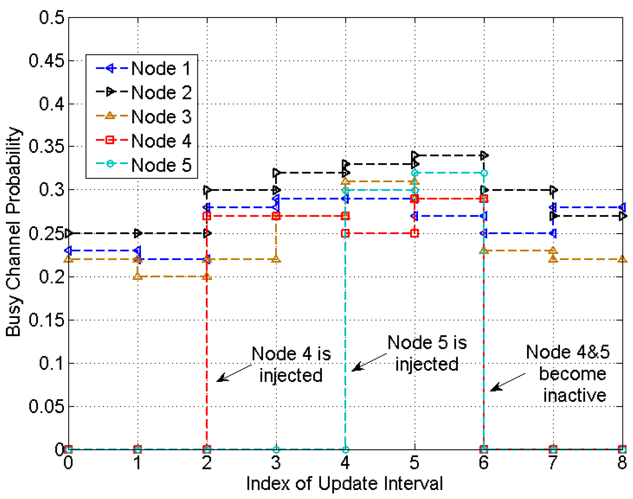
Figure 8 and
Figure 9 show the experimental results for a network with changes on the number of nodes. Initially Node 1, Node 2 and Node 3 are in the network with throughput demands of
,
,
, respectively. At the second update, Node 4 is injected with a throughput demand of
, followed by injection of Node 5 with a throughput demand of
at the 4th update. Node 4 and Node 5 become inactive at the 6th update. The update time is set to be 120 s and the threshold
is set to 0.02.
Figure 8.
Busy channel probability in a heterogeneous network with changes on the number of nodes.
Figure 8.
Busy channel probability in a heterogeneous network with changes on the number of nodes.
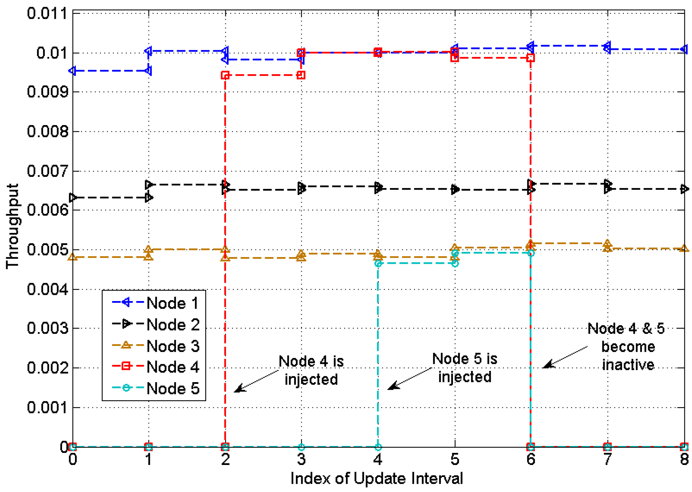
Figure 9.
Actual throughput in a heterogeneous network with changes on the number of nodes.
Figure 9.
Actual throughput in a heterogeneous network with changes on the number of nodes.
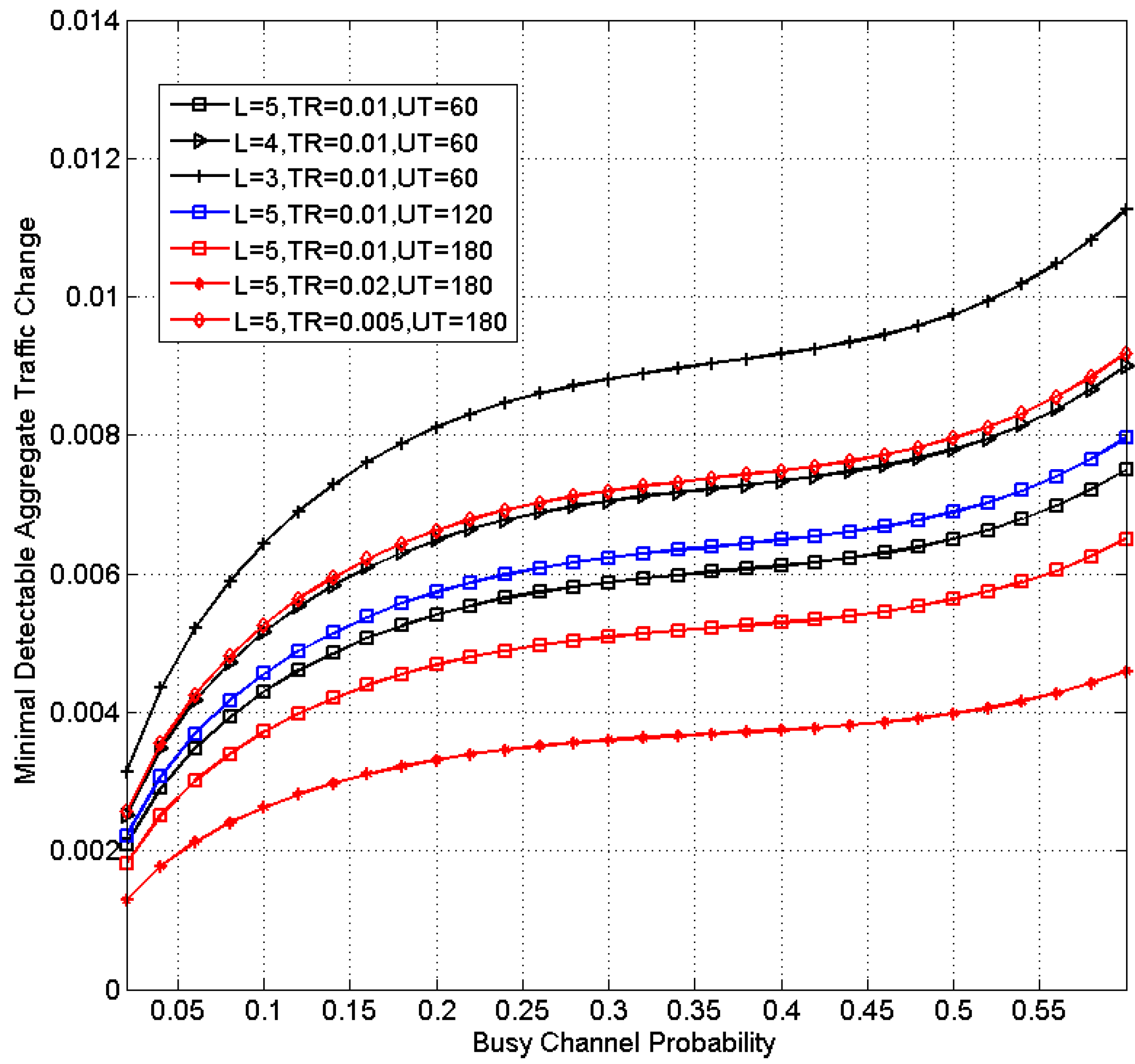
Figure 8 shows the results of busy channel probability (BCP). The BCPs of Node 1–3 changes significantly when Node 4 is injected, with an increment of 0.06, 0.05, 0.02, respectively. According to
Section 4, the change of BCP due to the injection of Node 4 is 0.0598 and the maximal fluctuations of the BCPs of the three without any traffic changes are 0.0234, 0.0287 and 0.0331, respectively. Node 3 with the lowest transmission rate suffers most from the noisy measurement of BCP. Nevertheless, as 0.0598 is greater than the maximal fluctuations and all nodes are able to detect the injection of Node 4. However, the detection of Node 5 is difficult as it brings a lower traffic. The BCPs do not change significantly. When Node 4 and Node 5 become inactive, the BCPs of the remaining nodes change significantly, with decrement of 0.02, 0.04 and 0.06.
Despite the fluctuations on BCP, each node is able to adjust the transmission rate to meet the throughput demand. The actual throughput is plotted in
Figure 9. It is observed that the average throughput of each node is very close to the demand, with an average percentage error of 0.875% at the optimal point.
6. Conclusions
This paper presents a fully distributed rate adjustment algorithm for heterogeneous CSMA/CA networks with time-varying traffics. The algorithm enables each node in the CSMA/CA network to tune its transmission rate to a desired level with respect to a given throughput demand without any central coordination.
The novelty of the proposed algorithm lies in the following three aspects. First, to the best knowledge of the authors, it is the first research work that provides a mathematical characterization of heterogeneous traffics in an IEEE 802.15.4 CSMA/CA network. By exploiting the CCA information, each participating node can accurately determine the level of contention in the network in terms of aggregate transmission rate. Second, with the knowledge of the traffics in the network, each node is able to estimate the packet success rate at equilibrium point and adjust the transmission rate to meet the throughput demand. Compared with existing methods that typically has a prediction error of several percent, the proposed algorithm only yields an average error of 0.43% for homogeneous networks and 0.524% for heterogeneous networks and does not require either complex modeling or central coordination. Third, the algorithm is more flexible in that it is robust against time-varying traffics and can adjust to a new transmission rate should there be any traffic changes.
The proposed algorithm can be used for both homogeneous and heterogeneous CSMA/CA networks. Particularly, it is most suitable for applications with certain throughput requirements. For example, in an intra-vehicular or intra-satellite control system, it is often required that every sensor send a minimum number of measurement packets to the controller to guarantee certain control performance. In this case, the algorithm can be employed to determine the actual transmission rate required. As for practical considerations, the proposed method simply makes use of CCA information and does not require modifications on the CSMA/CA protocol. It is thus easy to implement and computationally inexpensive with the use of a look-up table. Our implementation based on the TinyOS [
37,
39] platform also shows its compatibility with prevailing protocol stack.
It should be noted that the proposed algorithm can only be applied to IEEE 802.15.4-like CSMA/CA networks. The extension to other forms of CSMA/CA networks (e.g., IEEE 802.11) is possible but requires a different modeling approach, which is beyond the scope of this paper. It should also be noted that the proposed research considered a star-topology and the extension to other topologies is also beyond the scope of this paper.
Future works can be pursued in the following aspects. First, this paper considers each CCA result to be a binary value (
i.e., busy/idle). In fact, since each CCA may take up at most two slots and there are four possible outcomes, it is possible to obtain more information on the level of contention by further processing the results. This may also help to propose novel CCA strategies (e.g., the additional carrier sensing method shown in [
19]). It is also possible to take into account the imperfect carrier sensing into the modeling [
41]. Second, the combination of advanced estimation techniques such as extended Kalman filter and the proposed algorithm may help reduce the error. Third, for a distributed network, there are various forms of local information that can be exploited. For example, the acknowledgement packet (ACK) from the receiver also reflects how busy the network is. Combining the CCA with the ACK can better characterize the network condition. Fourth, in the experiment setup, this paper considers a typical laboratory environment where nodes are randomly placed among cubicles. Future works may consider other typical customized configurations and more extensive experiments can be performed. This may help test scenarios of hotspot as well as bottlenecks and identify potential performance issues in more detail. Lastly, as it is very common that IEEE 802.15.4 devices co-exist with IEEE802.11 (WiFi) networks, it would be practically significant to study the traffic characterization and transmission rate control in the presence of competing networks.


