
The Node Deployment of Intelligent Sensor Networks Based on the Spatial Difference of Farmland Soil

 ,
,
Abstract
:1. Introduction
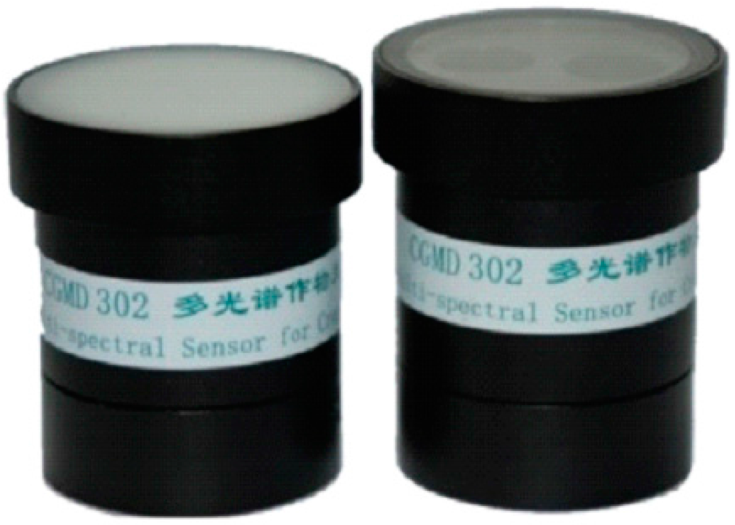
2. The CGMD302 Crop Growth Information Sensor
3. Fuzzy C-means Clustering
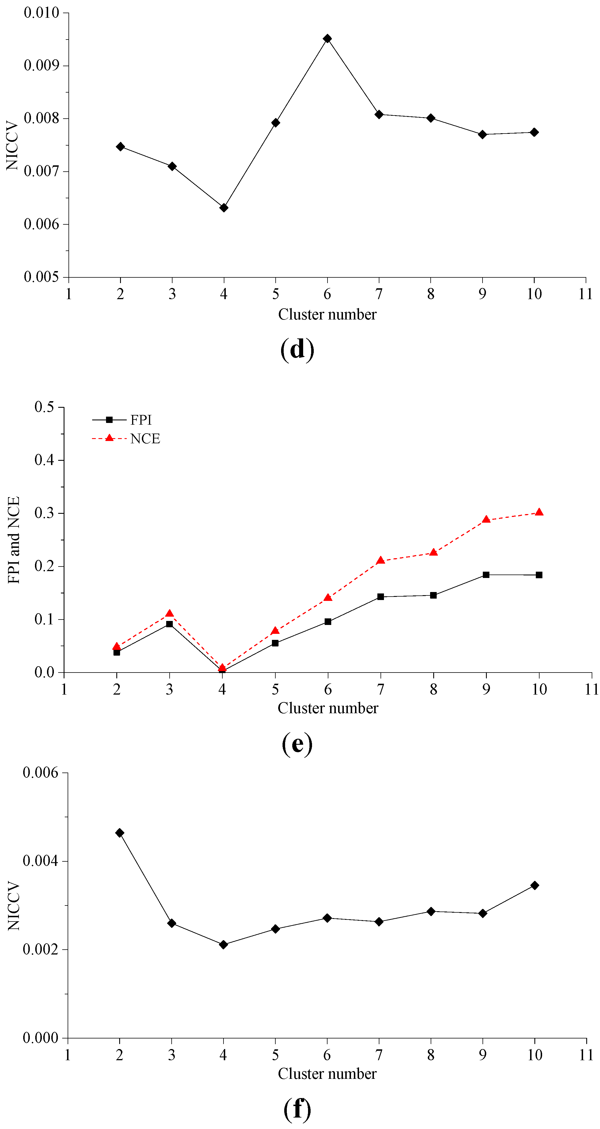
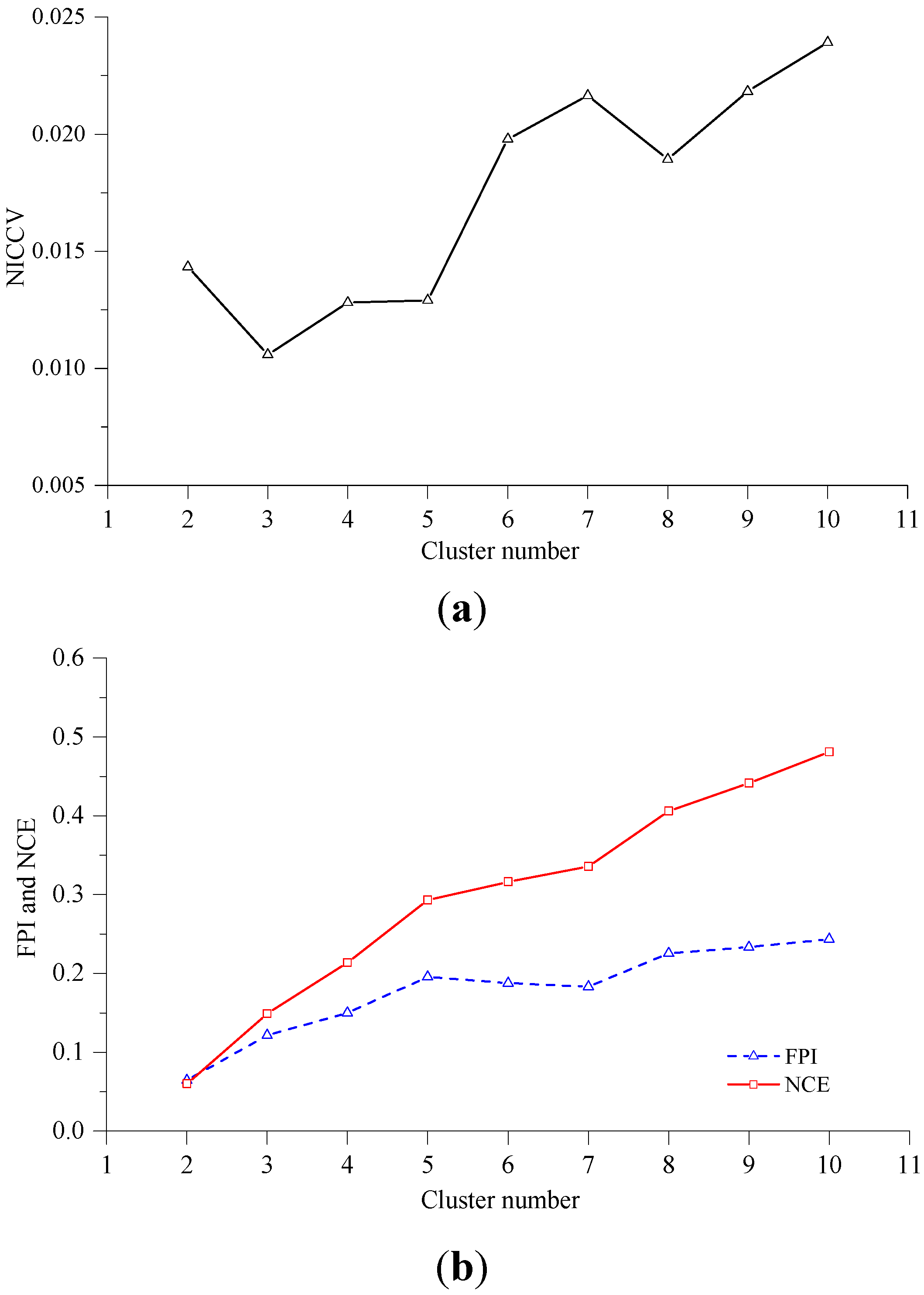
4. Cluster Validity
4.1. Normalized Intra-Cluster Coefficient of Variance
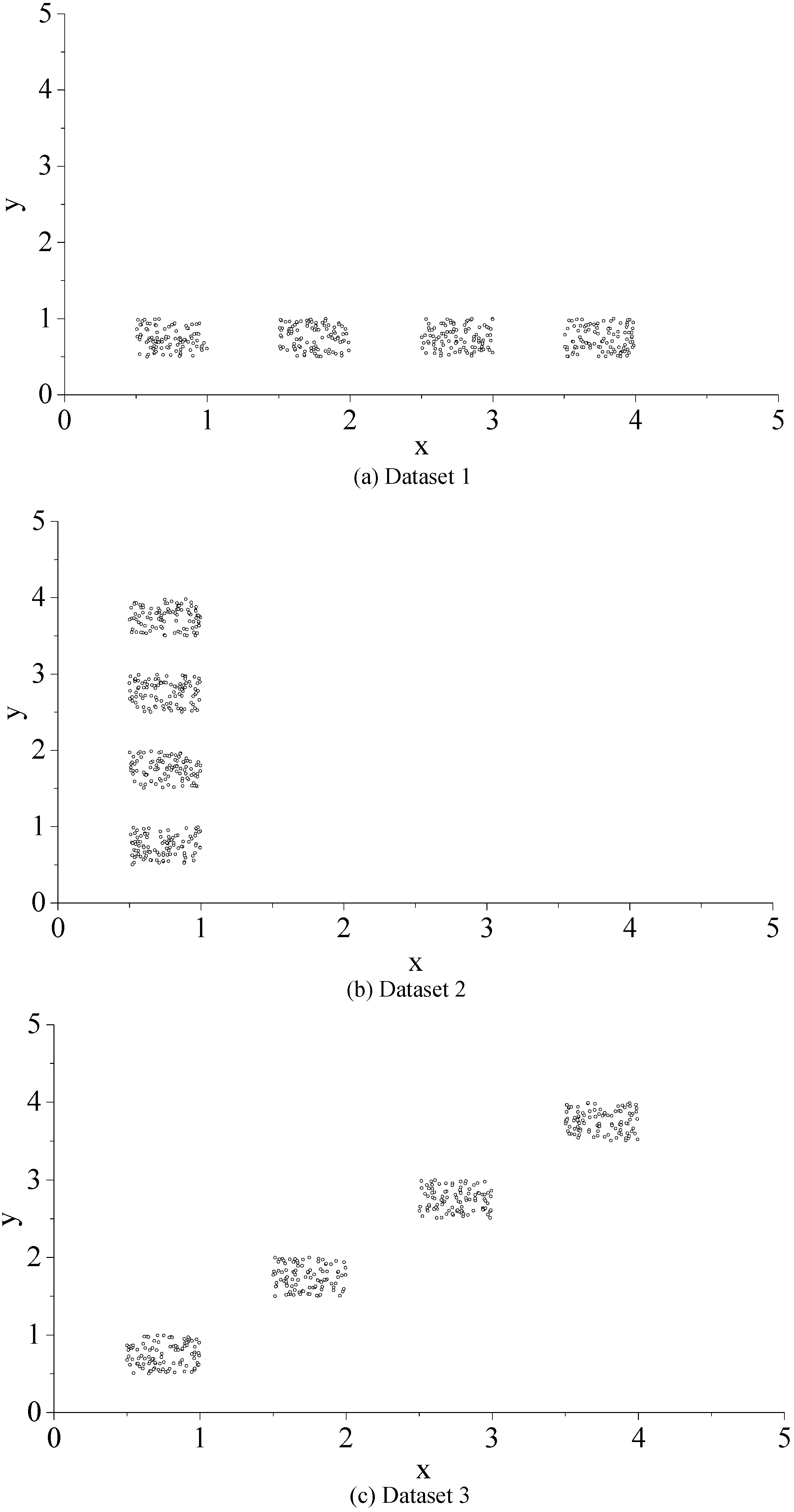
4.2. Verification


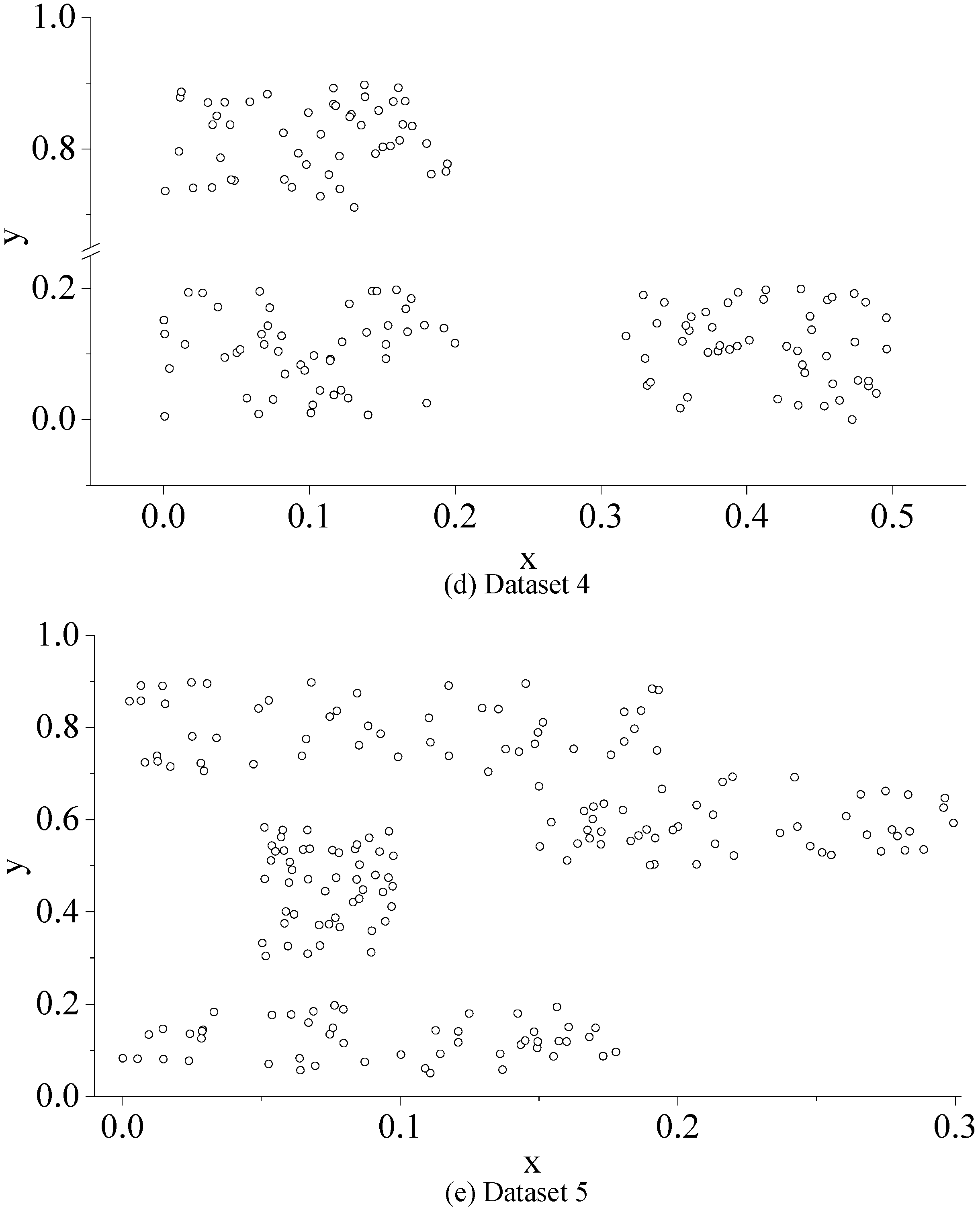
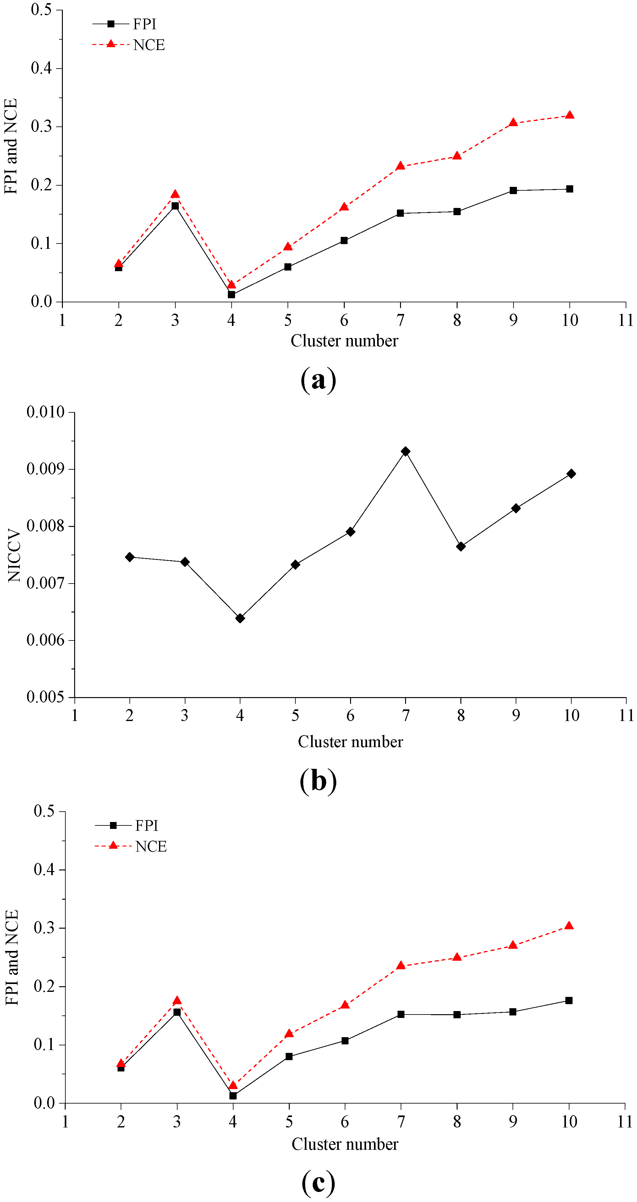
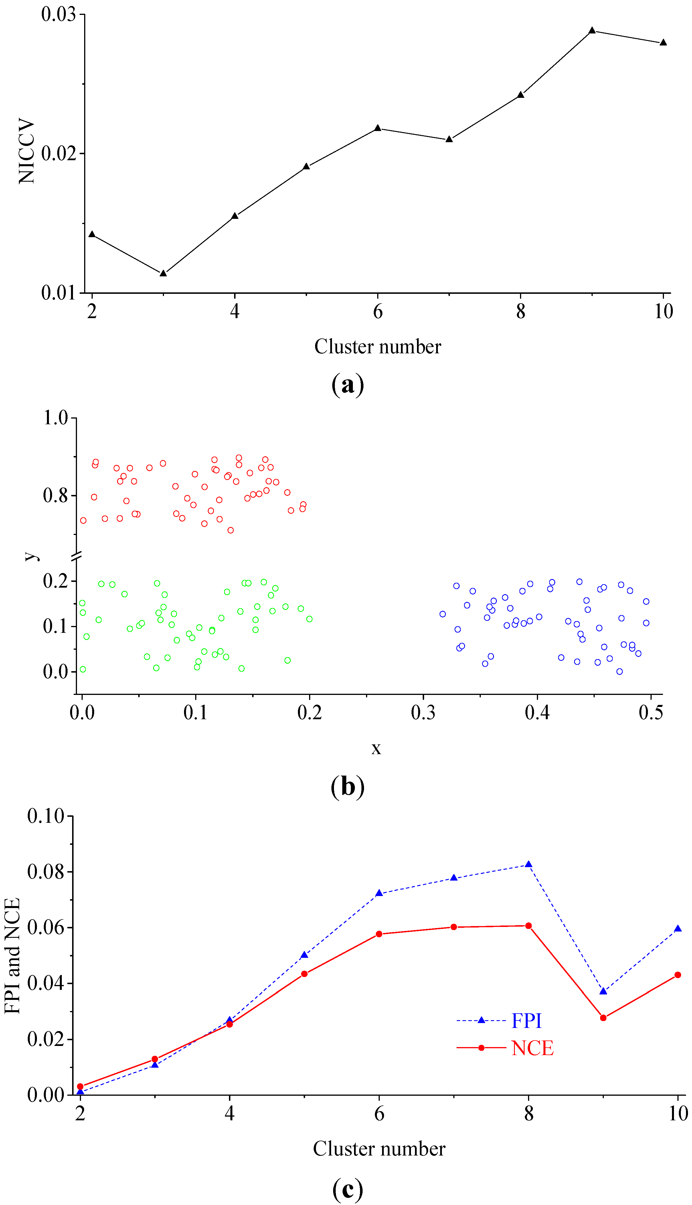
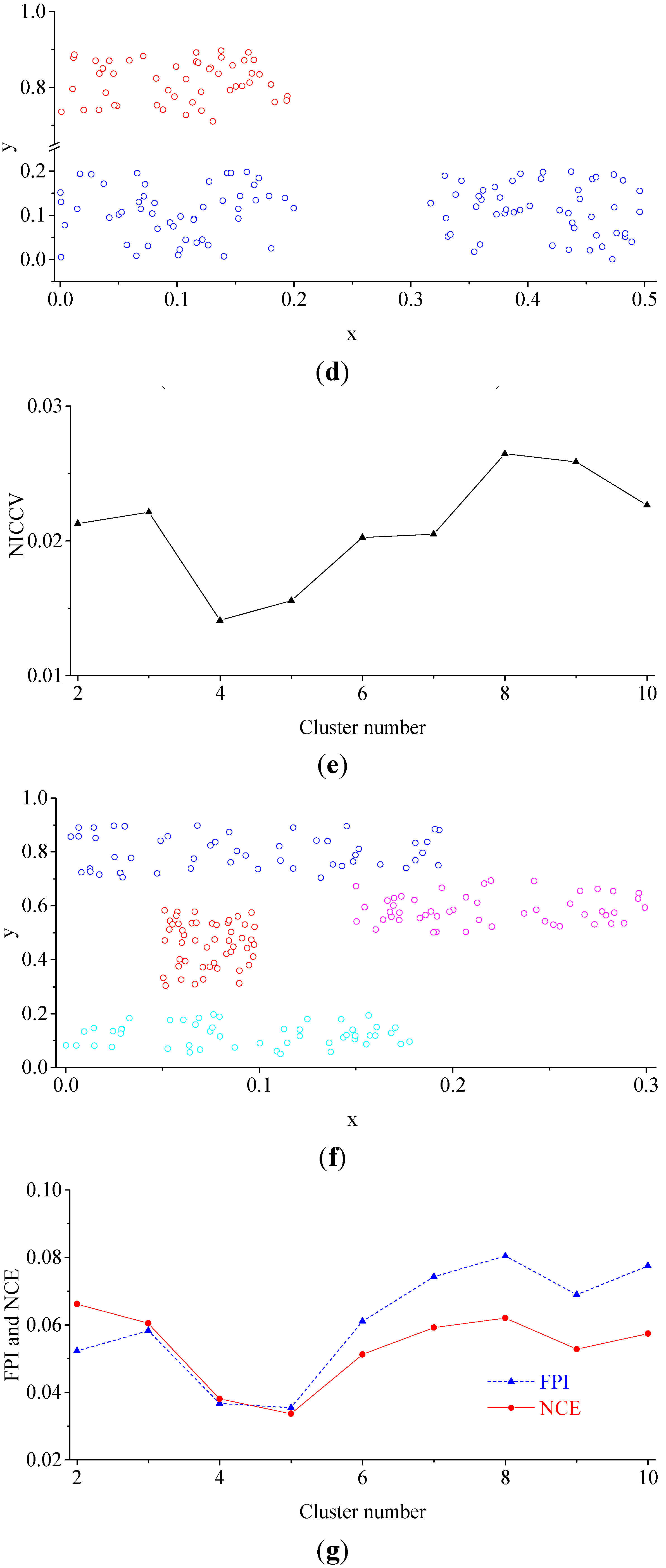
4.2.1. Experiment 1

4.2.2. Experiment 2


4.2.3. Experiment 3
4.2.4. The Sensitivity of Discriminant Functions to m


4.2.5. The Sensitivity of Discriminant Functions to the Number of Clusters c

5. Dividing the Farmland Based on the Spatial Difference of Soil Nutrients


| Soil Properties | Model | Semi-Variance Function Model Parameters | |||||
|---|---|---|---|---|---|---|---|
| Nugget | Sill | Nugget/Sill (%) | Range (m) | R2 | RSS | ||
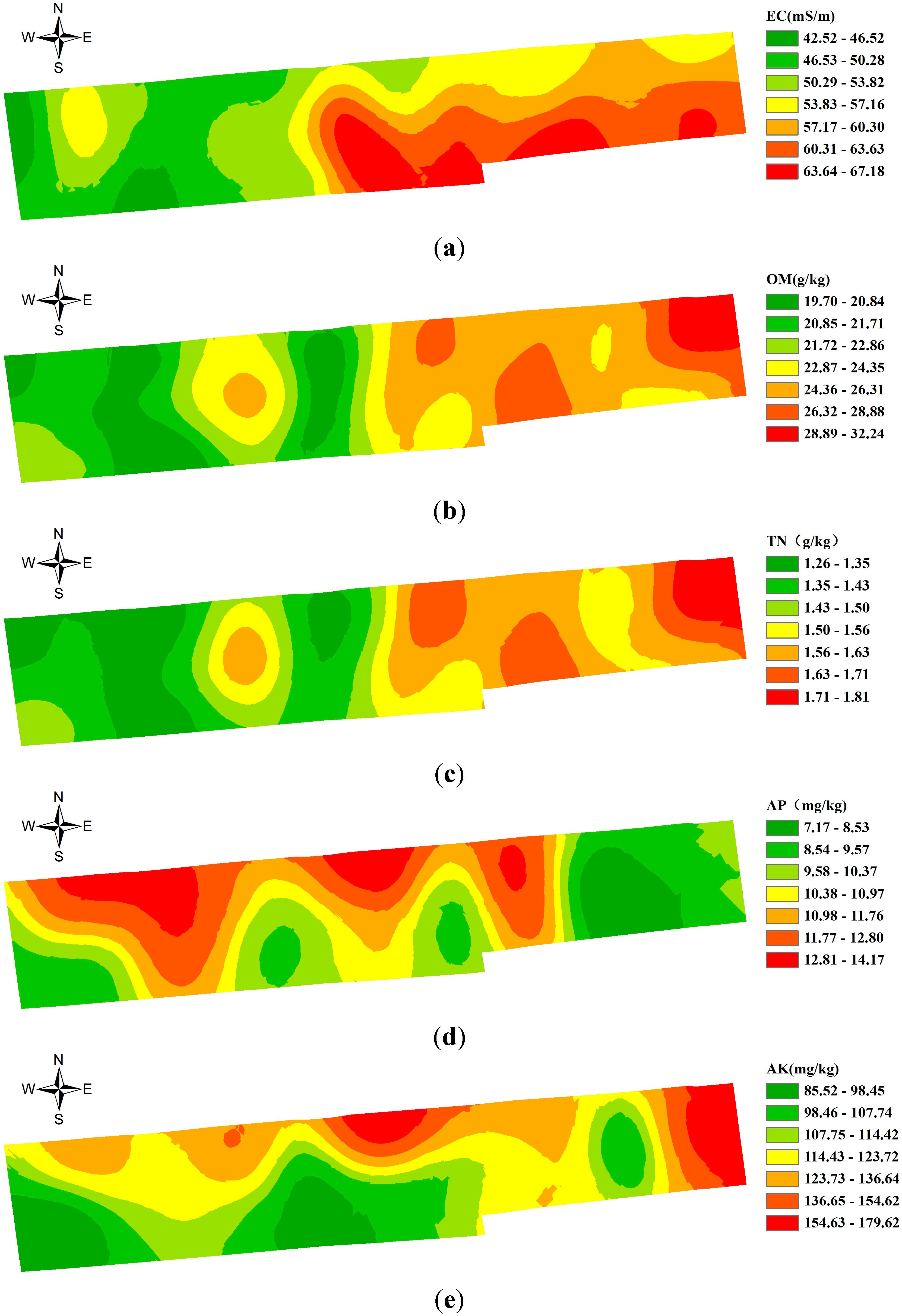
| EC (mS/m) | Spherical | 4.559 | 28.753 | 15.95 | 131.02 | 0.956 | 0.0157 |
| OM (g/kg) | Spherical | 0.0531 | 0.193 | 27.51 | 84.77 | 0.825 | 0.0038 |
| TN (g/kg) | Spherical | 1.52 × 10⁻⁴ | 3.31 × 10⁻⁴ | 45.92 | 91.23 | 0.869 | 0.0225 |
| AP (mg/kg) | Exponential | 3.85 | 7.701 | 49.99 | 149.7 | 0.908 | 0.0688 |
| AK (mg/kg) | Exponential | 4.50 × 10⁻⁴ | 0.072 | 0.63 | 65.2 | 0.873 | 0.0055 |
| Zones | EC | OM | TN | AP | AK | |||||
|---|---|---|---|---|---|---|---|---|---|---|
| Mean mS·m−1 | CV % | Mean g·kg−1 | CV % | Mean g·kg−1 | CV % | Mean mg·kg−1 | CV % | Mean mg·kg−1 | CV % | |
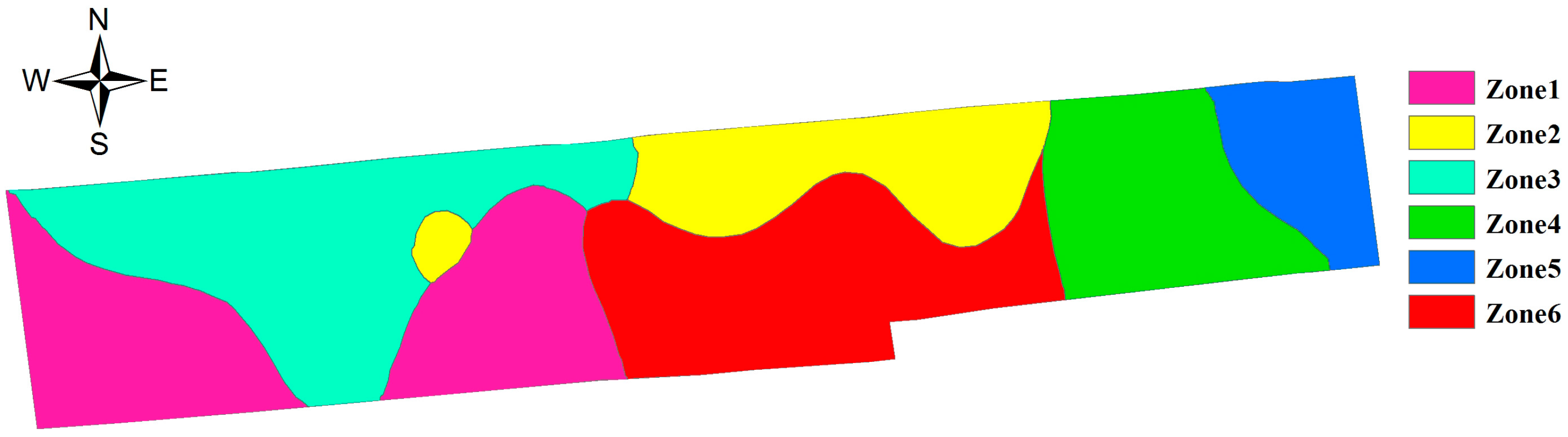
| Zone 1 | 49.43d | 9.59 | 21.54c | 12.63 | 1.401c | 12.60 | 9.46bc | 13.60 | 94.74d | 15.80 |
| Zone 2 | 55.38c | 4.42 | 25.28b | 11.42 | 1.590b | 11.08 | 12.67a | 22.73 | 144.39b | 26.34 |
| Zone 3 | 50.55d | 8.16 | 21.76c | 8.26 | 1.387c | 9.91 | 12.74a | 11.59 | 127.58bc | 22.95 |
| Zone 4 | 61.54ab | 4.28 | 24.39b | 8.59 | 1.549b | 8.20 | 8.12c | 23.82 | 116.57cd | 25.42 |
| Zone 5 | 58.5bc | 7.05 | 31.33a | 11.38 | 1.800a | 10.80 | 8.47c | 20.43 | 173.17a | 24.78 |
| Zone 6 | 63.8a | 6.55 | 24.73b | 12.62 | 1.580b | 10.67 | 10.52b | 20.90 | 110.00cd | 12.01 |
| total | 55.35 | 12.25 | 23.66 | 14.46 | 1.501 | 12.96 | 10.71 | 25.41 | 120.33 | 29.80 |
6. Comparing the Performance of Deployment Methods
7. Conclusions
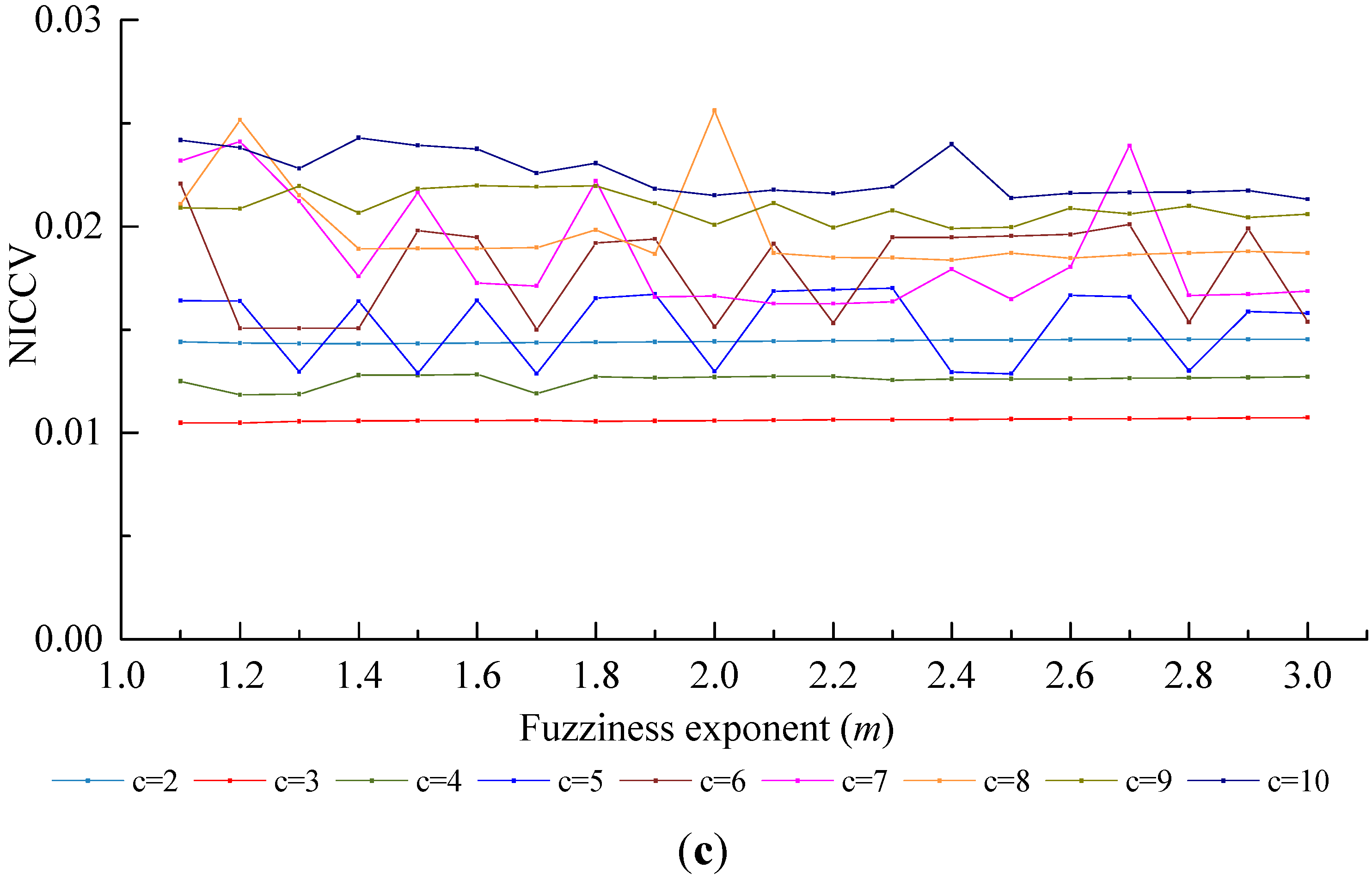
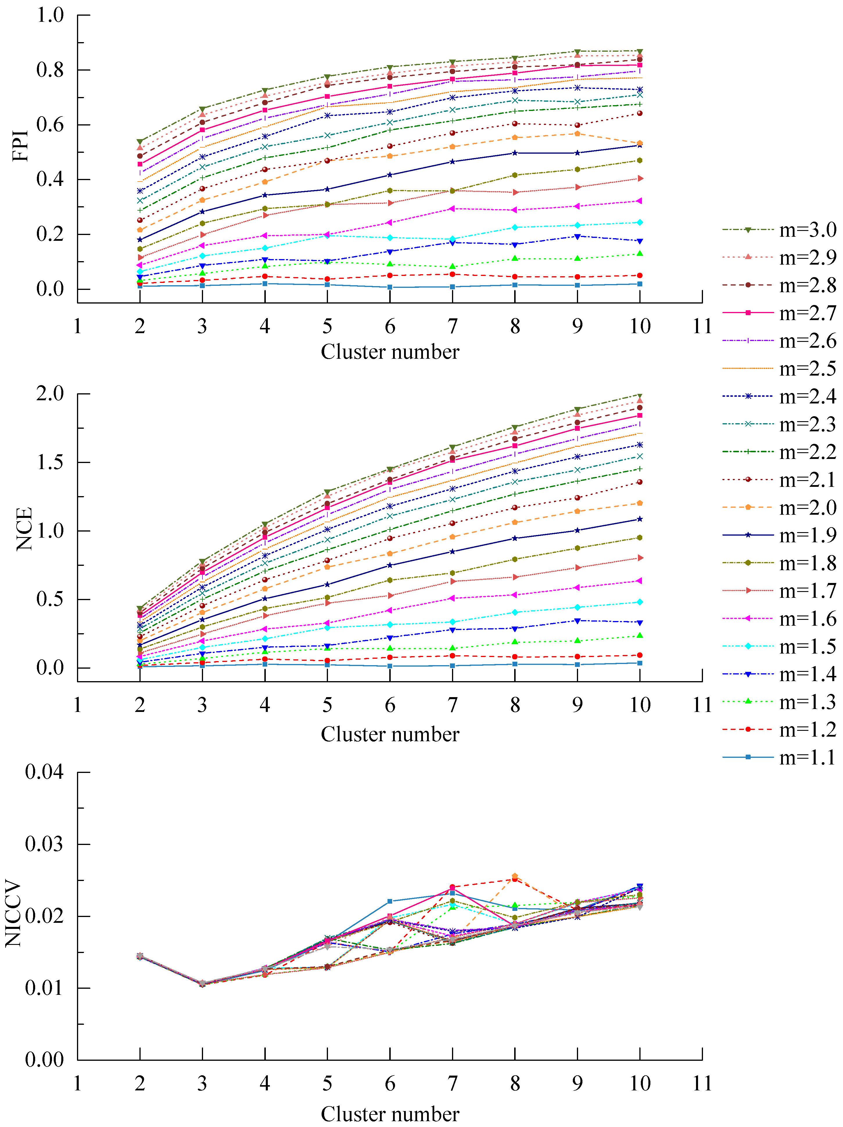
- In accordance with the farmland soil attribute data, including the organic matter content, total nitrogen content, available phosphorus content, available potassium content, electrical conductivity, etc., fuzzy c-means clustering algorithm was utilized to divide the farmland. In order to accurately judge the optimal cluster number of fuzzy c-means clustering, a discriminant function for NICCV was established. NICCV was constructed on the basis of the variation of the intra-cluster and inter-cluster data after clustering. It was verified that NICCV could provide the correct cluster number for the test data with both simple and complex spatial distribution by using simulation data and the Iris standard test data set. Moreover, its performance was obviously superior to that of FPI and NCE. As indicated by the sensitivity analysis, FPI, NCE and NICCV were sensitive to the number of clusters , i.e., all of them increased with the increase of . Besides, FPI and NCE showed a strong sensitivity to the fuzzy weighted exponent m, which suggests that both of them raised with the increasing . Moreover, when m was different, they might provide various optimal cluster numbers. On the contrary, NICCV was insensitive to . Thus, the NICCV with different cluster numbers still could be a horizontal line or fluctuate within a narrow range horizontally as changed.
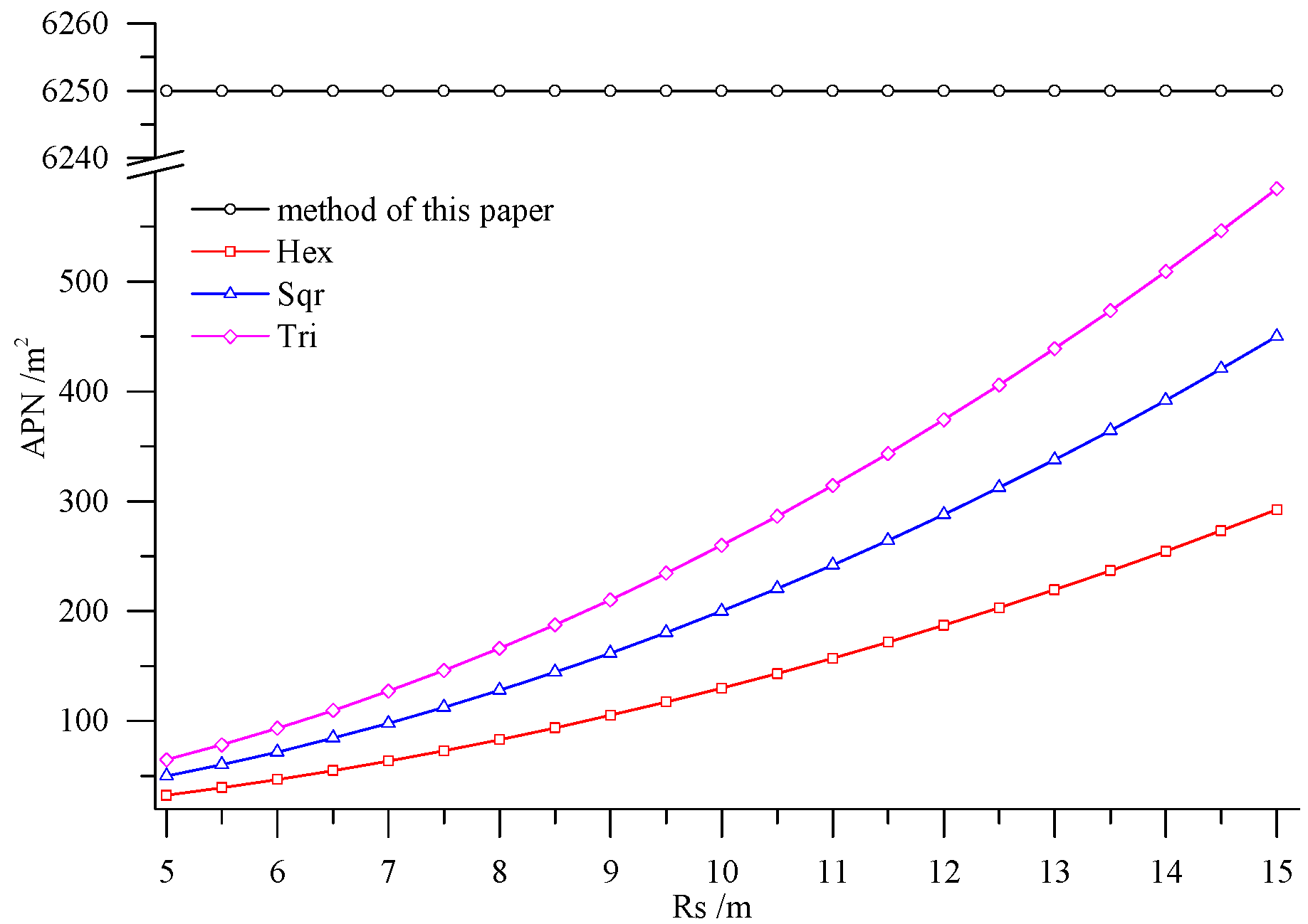
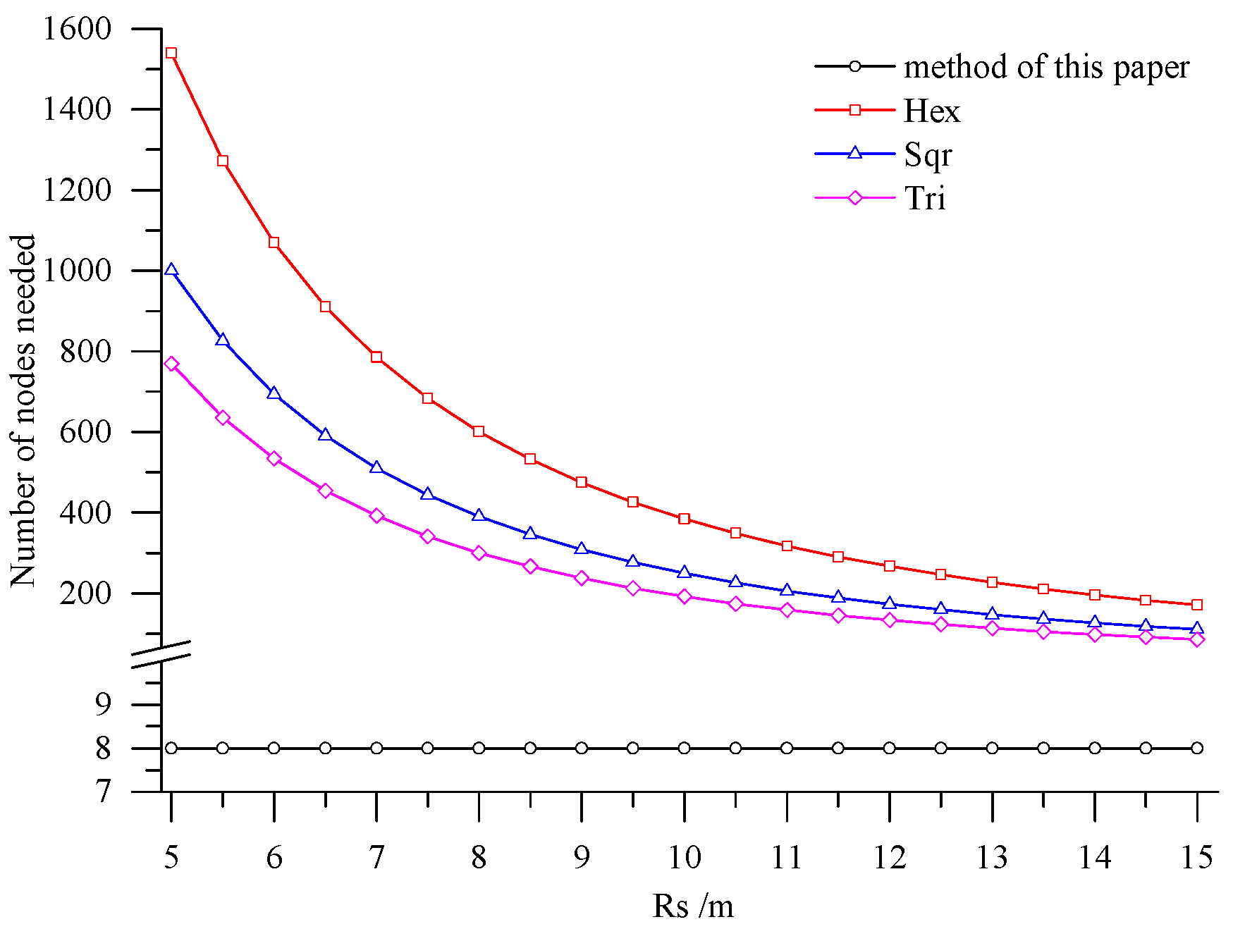
- Combining with the crop growth characteristics and features of sampling the crop growth information in farmland, the low-cost sensor node deployment was achieved based on the premise of completely monitoring the crop growth information. Compared with existing methods, the perception radius of sensor nodes did not need to be considered in this method. Through comparing the sensor node deployment for a farmland with an area of 5 hm2, it can be known that the APN of the method presented in this paper was 6250 m2, and only eight nodes were applied. However, when the perception radius of nodes was 15 m, the APNs of the deployed sensor networks based on the three kinds of regular grids, namely regular hexagon, square and equilateral triangle, were from 250 m2 to 600 m2, which suggests that 200–300 nodes were needed. In practical application, the perception radius of the sensors for crop growth information is relatively small. If the perception radius is 5 m, the APNs of the network deployed by the three regular grids are less than 100 m2, so that the number of required nodes is up to 800–1600, which means that deploying the sensor network nodes costs a lot. By comparison, it is demonstrated that the node deployment method in this paper is preferable in applications, which can guarantee the complete information monitoring and also minimize the node deployment costs.
- Crop growth is mainly influenced by soil nutrients; in addition, soil moisture and the NDVI of previous crop also have an important impact on crop growth. Information about soil moisture and NDVI can be obtained through sensors, NDVI can also be acquired through satellite remote sensing. If there is a large variation in the spatial distribution of soil moisture, it needs to be considered as one of the factors influencing farmland division. The ability of maintain soil water is given by its type, e.g., clay has a great ability to retain water, while the ability of sand is very limited. For this reason, soil type may substitute soil moisture as one of the criteria in dividing farmland. Different crops need different amounts of water and nutrients, as well as different times in the growing season. Furthermore, cropping system and crop phenology also affect crop growth. For this reason, our future work will consider all these factors in order to improve network deployment algorithm, so it can adapt to more complex application of wireless sensor network.
Acknowledgments
Author Contributions
Conflicts of Interest
References
- Gitelson, A.A.; Merzlyak, M.N. Remote sensing of chlorophyll concentration in higher plant leaves. Adv. Space Res. 1998, 22, 689–692. [Google Scholar] [CrossRef]
- Xue, L.H.; Yang, L.Z. Deriving leaf chlorophyll content of green-leafy vegetables from hyperspectral reflectance. ISPRS J. Photogramm. Remote Sens. 2009, 64, 97–106. [Google Scholar] [CrossRef]
- Castro, K.L.; Sanchez Azofeifa, G.A. Changes in spectral properties, chlorophyll content and internal mesophyll structure of senescing Populus balsamifera and Populus tremuloides leaves. Sensors 2008, 8, 51–69. [Google Scholar] [CrossRef]
- Yang, F.; Fan, Y.M.; Li, J.L.; Qian, Y.R.; Wang, Y.; Zhang, J. Estimating LAI and CCD of rice and wheat using hyperspectral remote sensing data. Trans. Chin. Soc. Agric. Eng. 2010, 26, 237–243. [Google Scholar]
- Li, Y.X.; Zhu, Y.; Dai, T.B.; Tian, Y.C.; Cao, W.X. Quantitative relationships between leaf area index and canopy reflectance spectra of wheat. Chin. J. Appl. Ecol. 2006, 17, 1443–1447. [Google Scholar]
- Huang, C.Y.; Wang, D.W.; Cao, L.P.; Zhang, Y.X.; Ren, L.T.; Cheng, C. Models for estimating cotton aboveground fresh biomass using hyperspectral data. Trans. Chin. Soc. Agric. Eng. 2007, 23, 131–135. [Google Scholar]
- Wang, D.C.; Wang, J.H.; Jin, N.; Wang, Q.; Li, C.J.; Huang, J.F.; Wang, Y.; Huang, F. ANN-based wheat biomass estimation using canopy hyperspectral vegetation indices. Trans. Chin. Soc. Agric. Eng. 2008, 24, 196–201. [Google Scholar]
- Evain, S.; Flexas, J.; Moya, I. A new instrument for passive remote sensing: 2. Measurement of leaf and canopy reflectance changes at 531 nm and their relationship with photosynthesis and chlorophyll fluorescence. Remote Sens. Environ. 2004, 91, 175–185. [Google Scholar] [CrossRef]
- Wang, X.; Zhao, C.J.; Zhou, H.C.; Liu, L.Y.; Wang, J.H.; Xue, X.Z.; Meng, Z.J. Development and experiment of portable NDVI instrument for estimating growth condition of winter wheat. Trans. Chin. Soc. Agric. Eng. 2004, 20, 95–98. [Google Scholar]
- Li, X.H.; Zhang, F.; Li, M.Z.; Zhao, R.J.; Li, S.Q. Design of a Four-waveband Crop Canopy Analyzer. Trans. Chin. Soc. Agric. Mach. 2011, 42, 169–173. [Google Scholar]
- Ni, J.; Wang, T.T.; Yao, X.; Cao, W.X.; Zhu, Y. Design and Experiments of Multi-spectral Sensor for Rice and Wheat Growth Information. Trans. Chin. Soc. Agric. Mach. 2013, 44, 207–212. [Google Scholar]
- Tan, W.J.; Wang, Y.Q.; Zhao, P.F.; Fan, L.F.; Huang, L.; Wang, Z.Y. Development of system for monitoring chlorophyll content of plant population using reflectance spectroscopy. Trans. Chin. Soc. Agric. Eng. 2014, 30, 160–166. [Google Scholar]
- Bekmezci, I.; Alagoz, F. Energy Efficient, Delay Sensitive, Fault Tolerant Wireless Sensor Network for Military Monitoring. Int. J. Distrib. Sens. Netw. 2009, 5, 729–747. [Google Scholar] [CrossRef]
- Kafi, M.A.; Challal, Y.; Djenouri, D.; Bouabdallah, A.; Khelladi, L.; Badache, N. A study of Wireless Sensor Network Architectures and Projects for Traffic Light Monitoring. Procedia Comput. Sci. 2012, 10, 543–552. [Google Scholar] [CrossRef]
- Vairamani, K.; Mathivanan, N.; Venkatesh, K.A.; Kumar, U.D. Environmental parameter monitoring using wireless sensor network. Instrum. Exp. Tech. 2013, 56, 468–471. [Google Scholar] [CrossRef]
- Díaz, S.E.; Pérez, J.C.; Mateos, A.C.; Marinescu, M.; Guerra, B.B. A novel methodology for the monitoring of the agricultural production process based on wireless sensor networks. Comput. Electron. Agric. 2011, 76, 252–265. [Google Scholar] [CrossRef]
- Burrell, J.; Brooke, T.; Beckwith, R. Vineyard computing: Sensor networks in agricultural production. IEEE Pervasive Comput. 2004, 3, 38–45. [Google Scholar] [CrossRef]
- Xiao, K.H.; Xiao, D.Q.; Luo, X.W. Smart water-saving irrigation system in precision agriculture based on wireless sensor network. Trans. Chin. Soc. Agric. Eng. 2010, 26, 170–175. [Google Scholar]
- Srbinovska, M.; Gavrovski, C.; Dimcev, V.; Krkoleva, A.; Borozan, V. Environmental parameters monitoring in precision agriculture using wireless sensor networks. J. Clean. Prod. 2015, 88, 297–307. [Google Scholar] [CrossRef]
- Abd El-kader, S.M.; Mohammad El-Basioni, B.M. Precision farming solution in Egypt using the wireless sensor network technology. Egypt. Inform. J. 2013, 14, 221–233. [Google Scholar] [CrossRef]
- Bai, X.L.; Kumar, S.; Xuan, D.; Yun, Z.Q.; Lai, T. Deploying wireless sensors to achieve both coverage and connectivity. In Proceedings of the 7th ACM International Symposium on Mobile Ad Hoc Networking and Computing, Florence, Italy, 22–25 May 2006; pp. 131–142.
- Wang, D.J.; Lin, L.W.; Xu, L. A study of subdividing hexagon-clustered WSN for power saving: Analysis and simulation. Ad Hoc Netw. 2011, 9, 1302–1311. [Google Scholar] [CrossRef]
- Liao, W.H.; Kao, Y.C.; Li, Y.S. A sensor deployment approach using glowworm swarm optimization algorithm in wireless sensor networks. Expert Syst. Appl. 2011, 38, 12180–12188. [Google Scholar] [CrossRef]
- Zou, Y.; Chakrabarty, K. Sensor deployment and target localization based on virtual forces. In Proceedings of the INFOCOM 2003. Twenty-Second Annual Joint Conference of the IEEE Computer and Communications, IEEE Societies, San Francisco, CA, USA, 30 March–3 April 2003; pp. 1293–1303.
- Chakrabarty, K.; Iyengar, S.S.; Qi, H.R.; Cho, E.C. Grid coverage for surveillance and target location in distributed sensor networks. IEEE Trans. Comput. 2002, 51, 1448–1453. [Google Scholar] [CrossRef]
- Aitsaadi, N.; Achir, N.; Boussetta, K.; Pujolle, G. Artificial potential field approach in WSN deployment: Cost, QoM, connectivity, and lifetime constraints. Comput. Netw. 2011, 55, 84–105. [Google Scholar] [CrossRef]
- Odeh, I.; Chittleborough, D.J.; McBratney, A.B. Soil pattern recognition with fuzzy-c-means: Application to classification and soil-landform interrelationships. Soil Sci. Soc. Am. J. 1992, 56, 505–516. [Google Scholar] [CrossRef]
- Moral, F.J.; Terron, J.M.; Silva, J.R. Delineation of management zones using mobile measurements of soil apparent electrical conductivity and multivariate geostatistical techniques. Soil Tillage Res. 2010, 106, 335–343. [Google Scholar] [CrossRef]
- Sun, X.L.; Zhao, Y.G.; Wang, H.L.; Yang, L.; Qin, C.Z.; Zhu, A.X.; Zhang, G.L.; Pei, T.; Li, B.L. Sensitivity of digital soil maps based on FCM to the fuzzy exponent and the number of clusters. Geoderma 2012, 171–172, 24–34. [Google Scholar] [CrossRef]
- Bezdek, J.C. Cluster Validity with Fuzzy Sets. J. Cybern. 1973, 3, 58–73. [Google Scholar] [CrossRef]
- Roubens, M. Fuzzy clustering algorithms and their cluster validity. Eur. J. Oper. Res. 1982, 10, 294–301. [Google Scholar] [CrossRef]
- Milligan, G.W. Clustering validation: Results and implications for applied analysis. In Clustering and Classification; Arabie, P., Hubert, L.J., de Soete, G., Eds.; Word Scientific: Singapore, 1996; pp. 341–375. [Google Scholar]
- Bragato, G. Fuzzy continuous classification and spatial interpolation in conventional soil survey for soil mapping of the lower Piave plain. Geoderma 2004, 118, 1–16. [Google Scholar] [CrossRef]
- De Bruin, S.; Stein, A. Soil-landscape modeling using fuzzy c-means clustering of attribute data derived from a digital elevation model (DEM). Geoderma 1998, 83, 17–33. [Google Scholar] [CrossRef]
- Fridgen, J.J.; Kitchen, N.R.; Sudduth, K.A.; Drummond, S.T.; Wiebold, W.J.; Fraisse, C.W. Management Zone Analyst (MZA). Agron. J. 2004, 96, 100–108. [Google Scholar] [CrossRef]
- Wu, M.L.; Wang, Y.S.; Sun, C.C.; Wang, H.L.; Dong, J.D.; Han, S.H. Identification of anthropogenic effects and seasonality on water quality in Daya Bay, South China Sea. J. Environ. Manag. 2009, 90, 3082–3090. [Google Scholar] [CrossRef] [PubMed]
- Windham, M.P. Cluster Validity for the Fuzzy c-Means Clustering Algorithrm. IEEE Trans. Pattern Anal. Mach. Intell. 1982, pami-4, 357–363. [Google Scholar] [CrossRef]
- Windham, M.P. Cluster validity for fuzzy clustering algorithms. Fuzzy Sets Syst. 1981, 5, 177–185. [Google Scholar] [CrossRef]
© 2015 by the authors; licensee MDPI, Basel, Switzerland. This article is an open access article distributed under the terms and conditions of the Creative Commons Attribution license (http://creativecommons.org/licenses/by/4.0/).
Share and Cite
Liu, N.; Cao, W.; Zhu, Y.; Zhang, J.; Pang, F.; Ni, J. The Node Deployment of Intelligent Sensor Networks Based on the Spatial Difference of Farmland Soil. Sensors 2015, 15, 28314-28339. https://doi.org/10.3390/s151128314
Liu N, Cao W, Zhu Y, Zhang J, Pang F, Ni J. The Node Deployment of Intelligent Sensor Networks Based on the Spatial Difference of Farmland Soil. Sensors. 2015; 15(11):28314-28339. https://doi.org/10.3390/s151128314
Chicago/Turabian StyleLiu, Naisen, Weixing Cao, Yan Zhu, Jingchao Zhang, Fangrong Pang, and Jun Ni. 2015. "The Node Deployment of Intelligent Sensor Networks Based on the Spatial Difference of Farmland Soil" Sensors 15, no. 11: 28314-28339. https://doi.org/10.3390/s151128314