
Kinematic Model-Based Pedestrian Dead Reckoning for Heading Correction and Lower Body Motion Tracking

Abstract
:1. Introduction
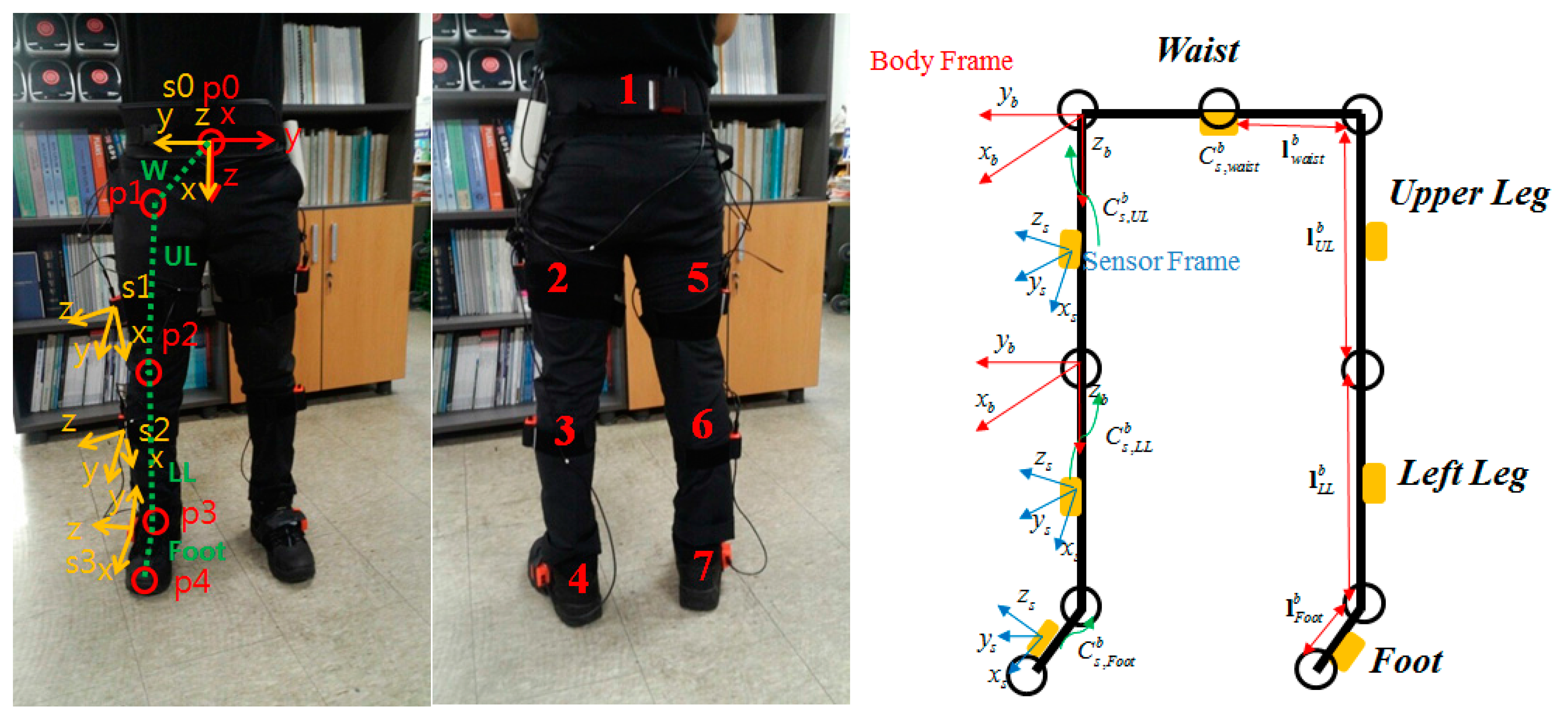
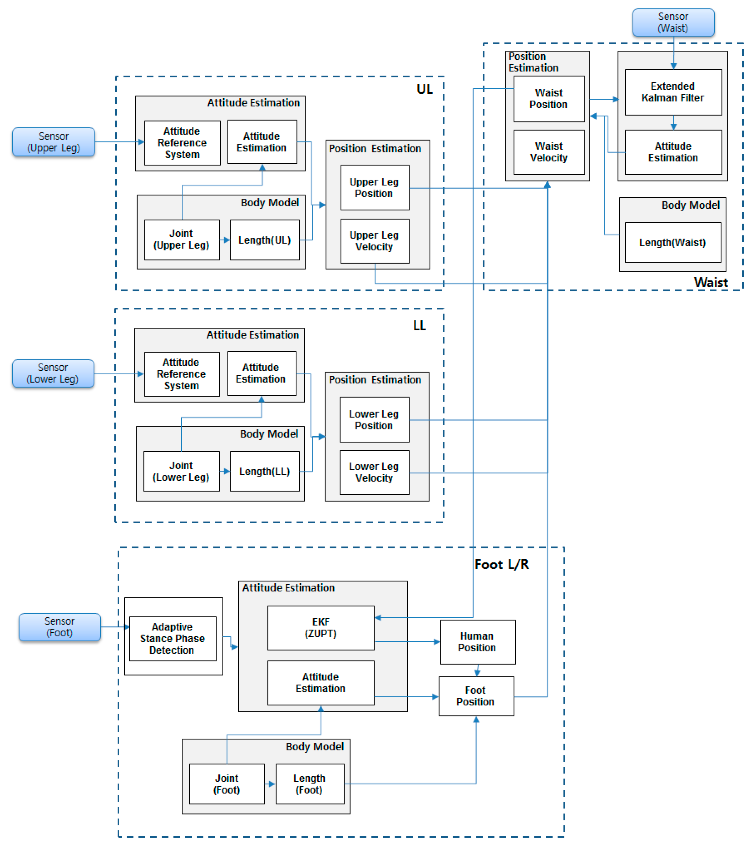
2. System Overview
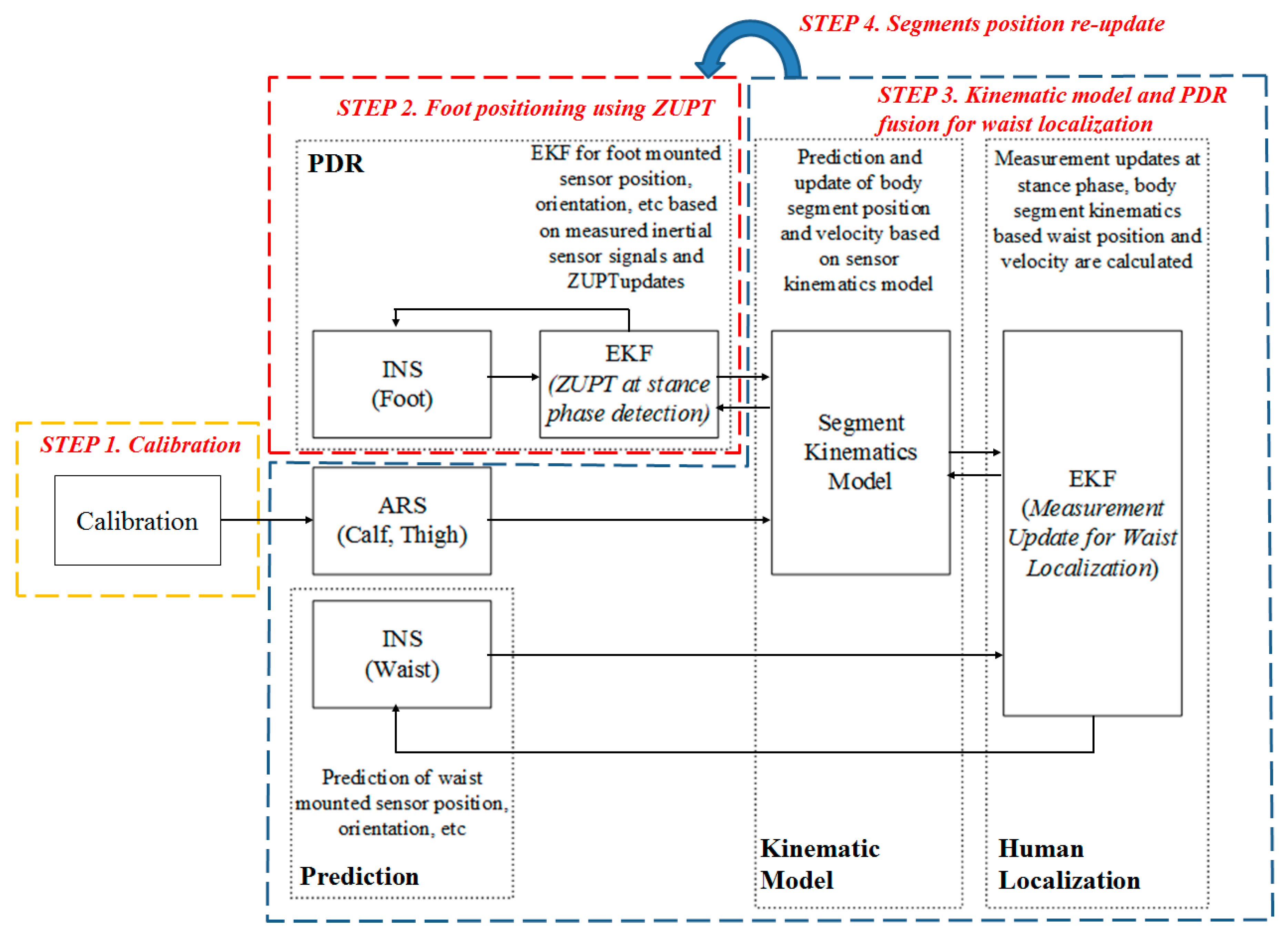
3. EKF-Based PDR and Kinematic Model Fusion
3.1. Calibration


3.2. Foot Positioning Using ZUPT

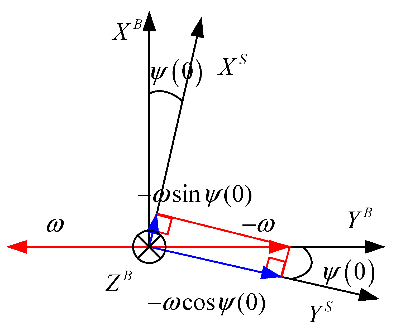
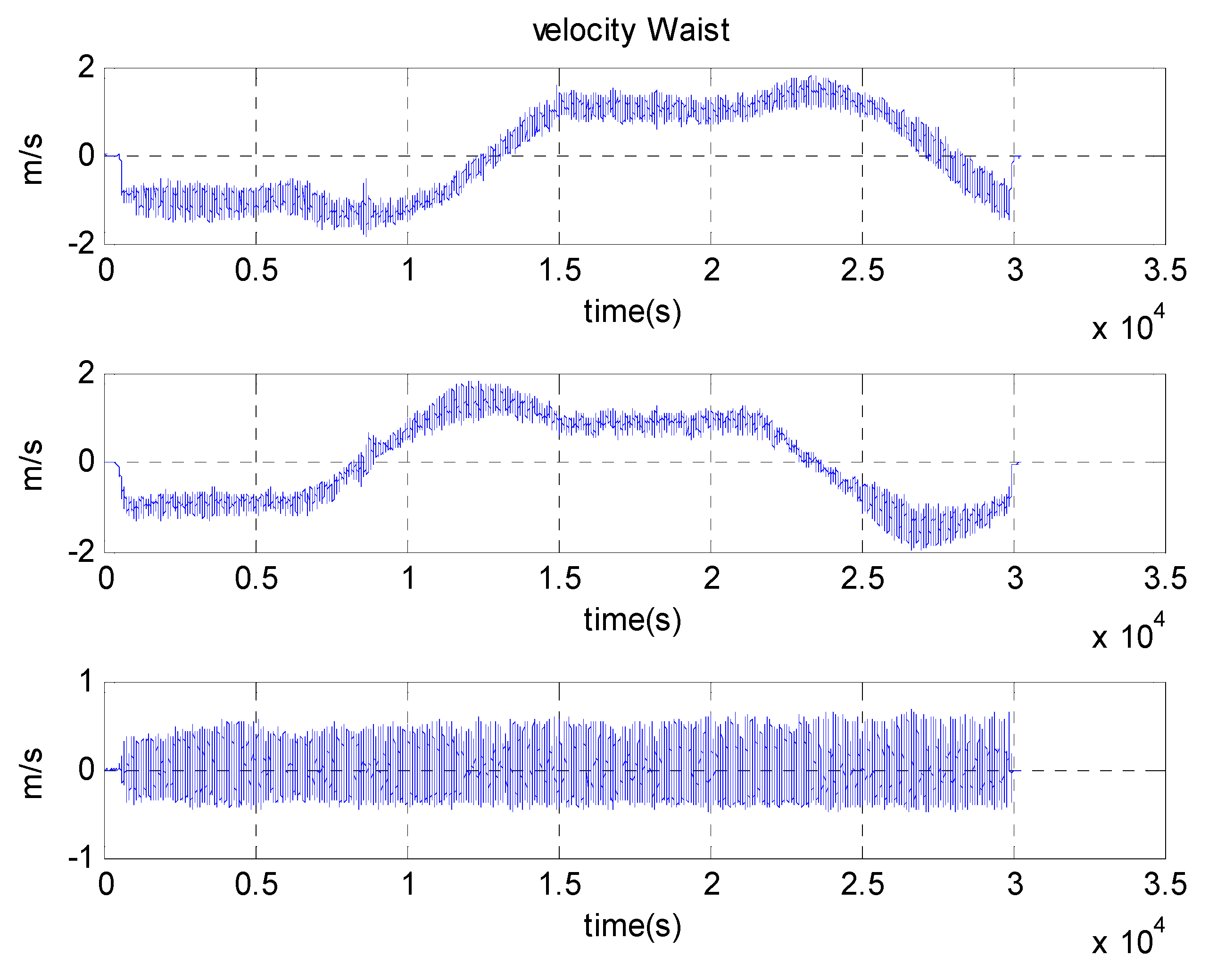
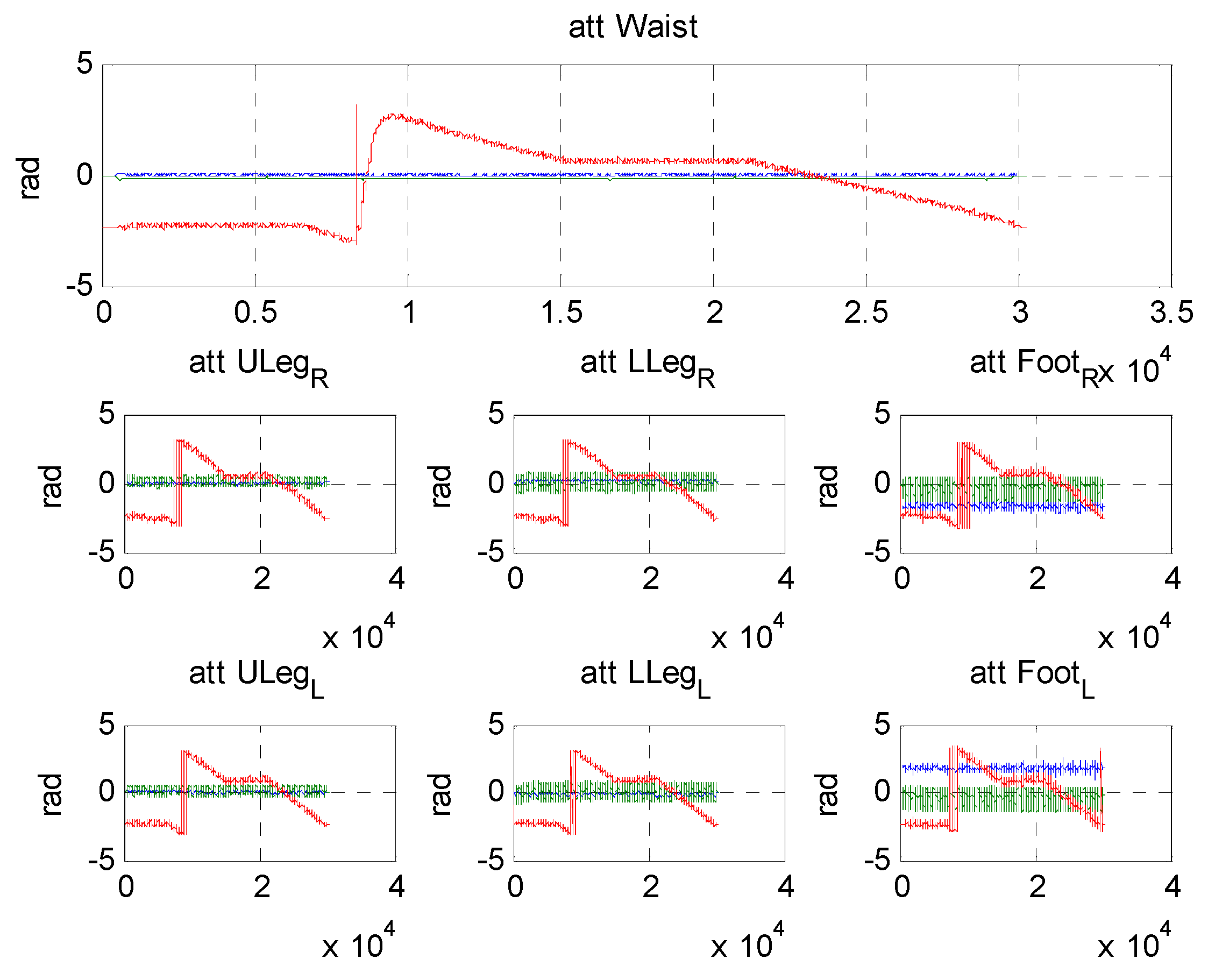
3.3. Kinematic Model and PDR Fusion for Waist Localization

3.4. Segments Position Re-Update
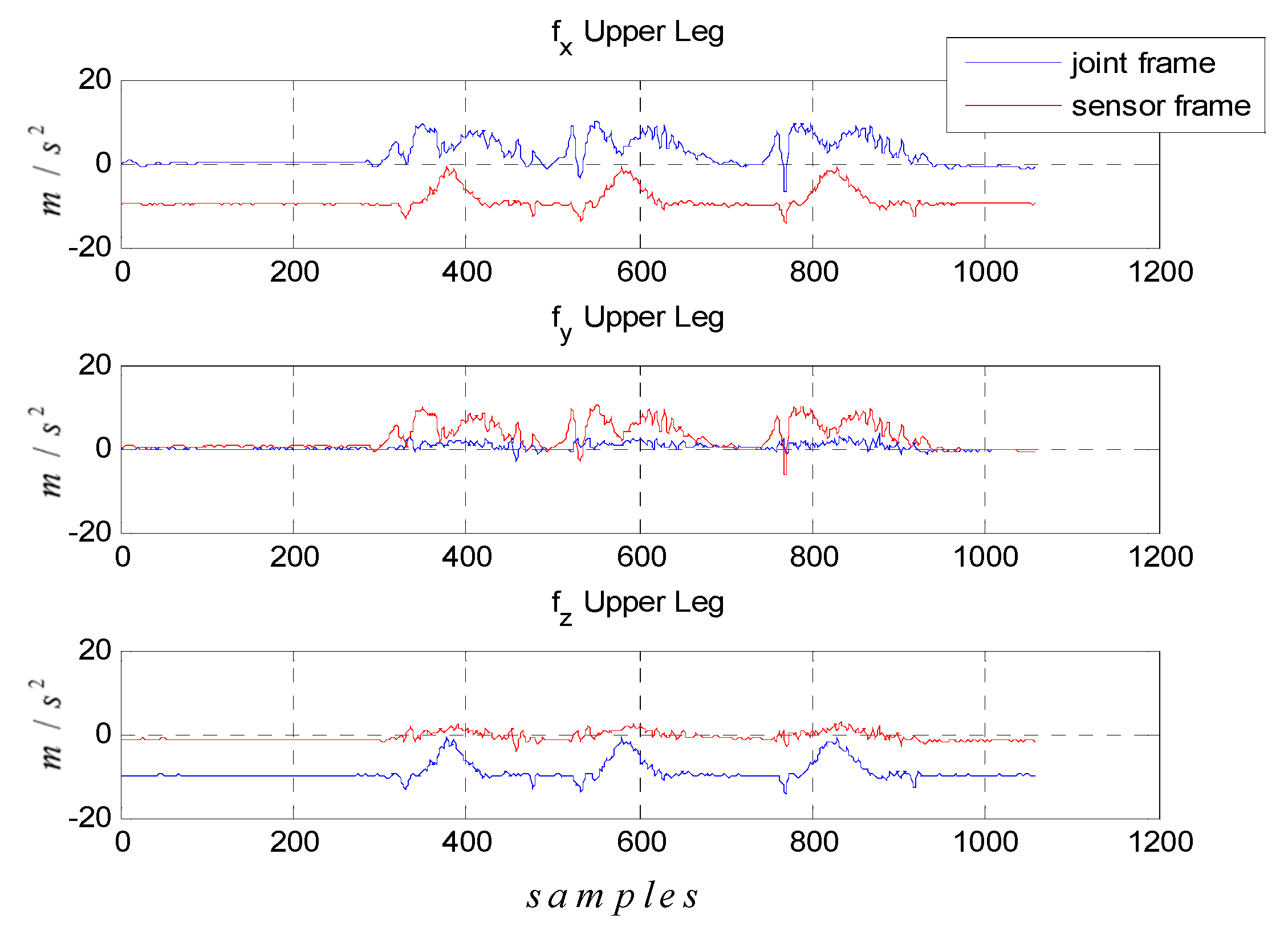
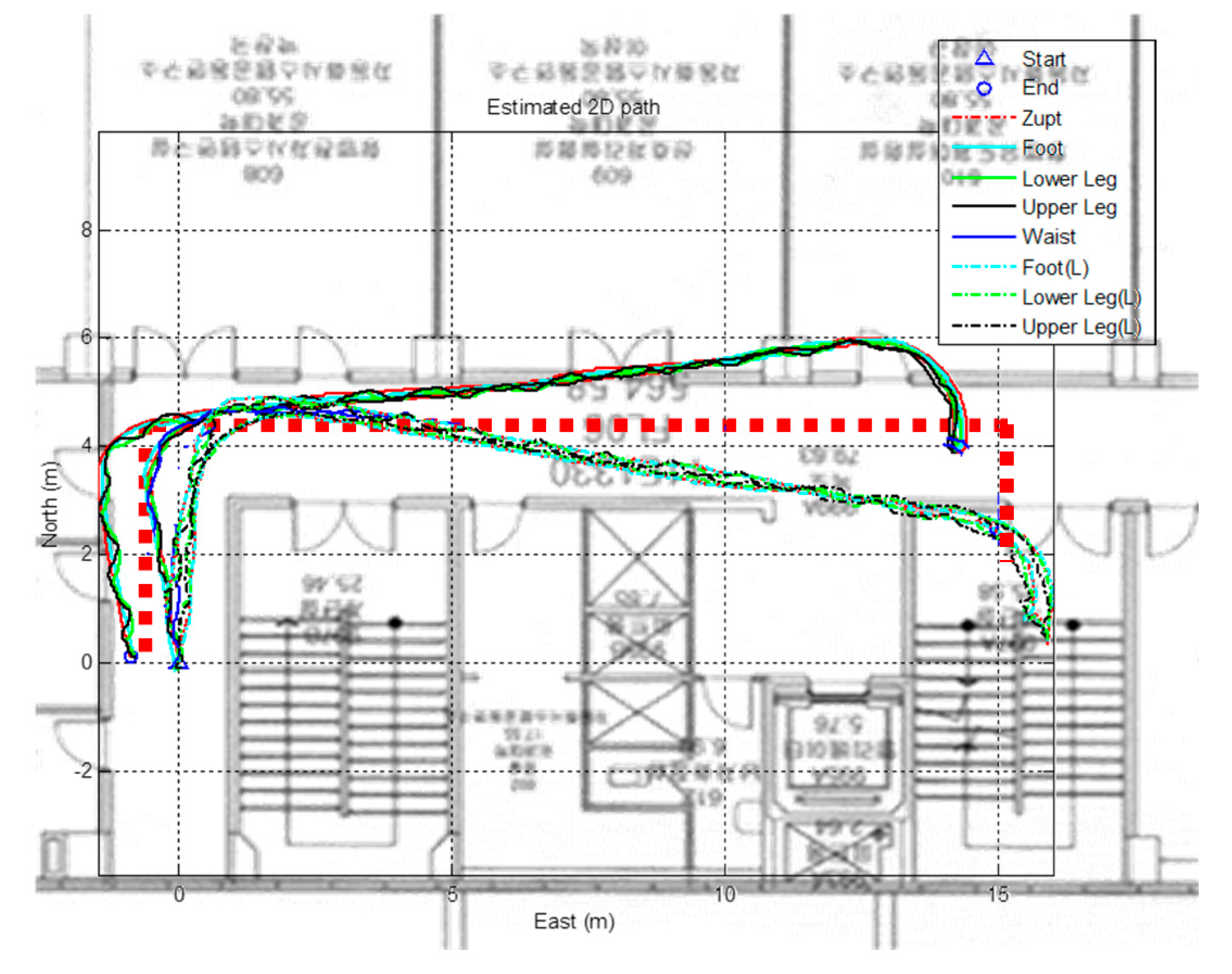
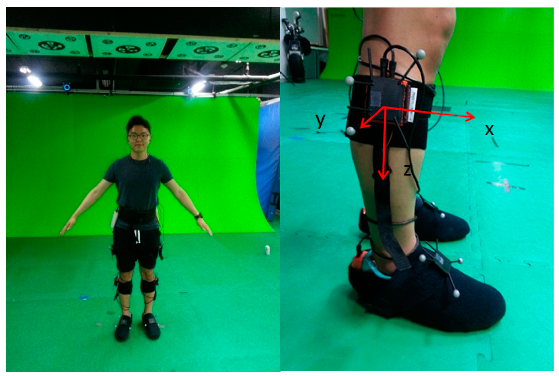
4. Experimental Results


| ZUPT | Proposed Algorithm | ||
|---|---|---|---|
| Right Foot | Left Foot | Waist | |
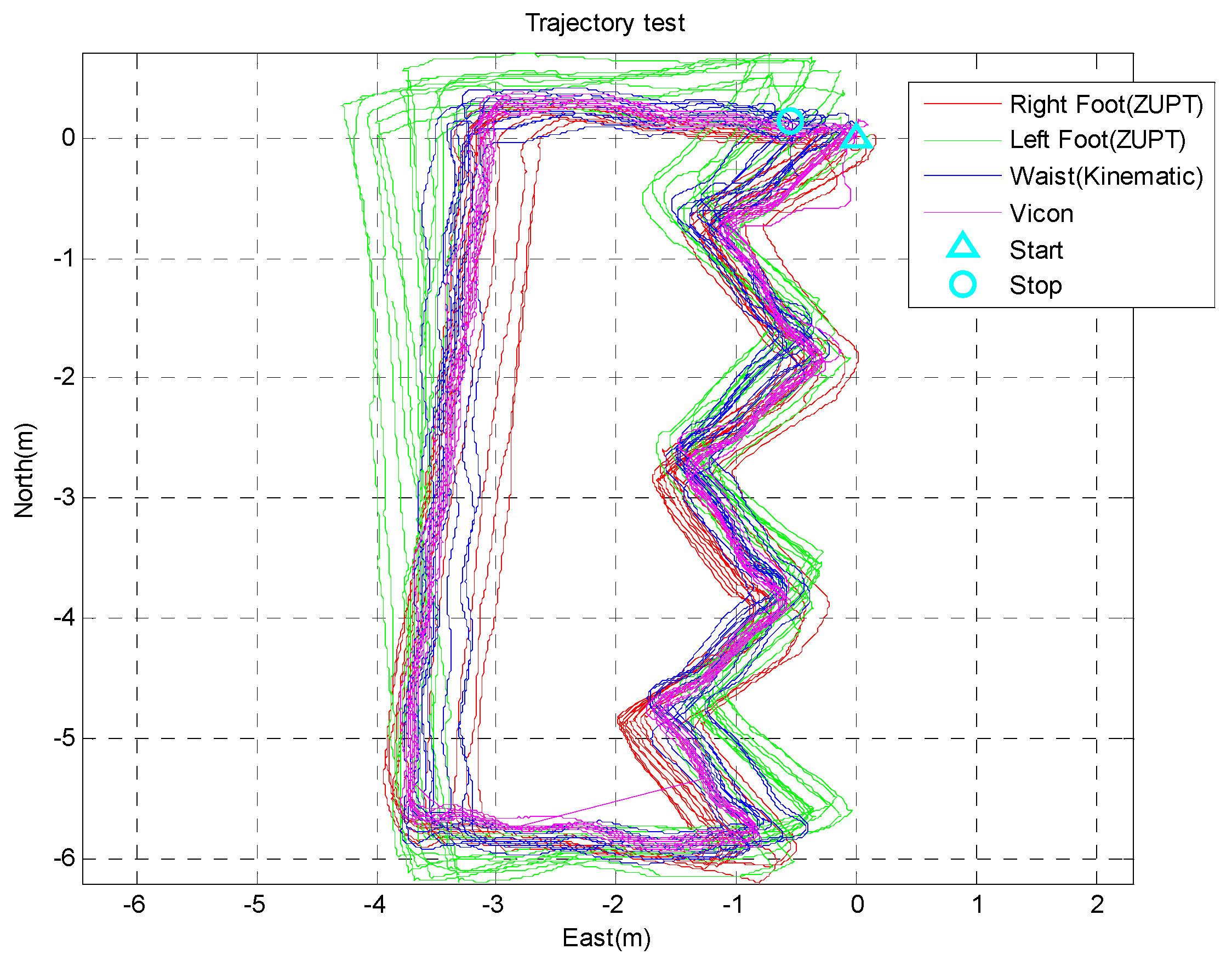
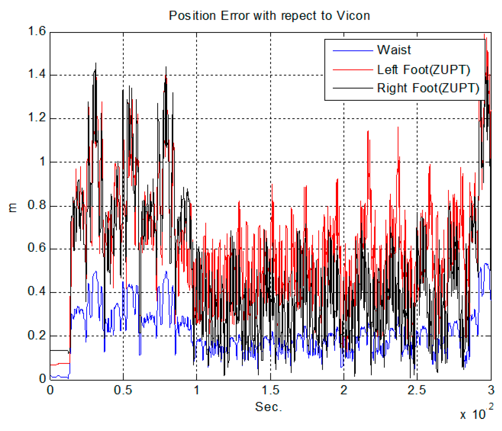
| Average position error (m) | 0.4934 | 0.6033 | 0.2085 |

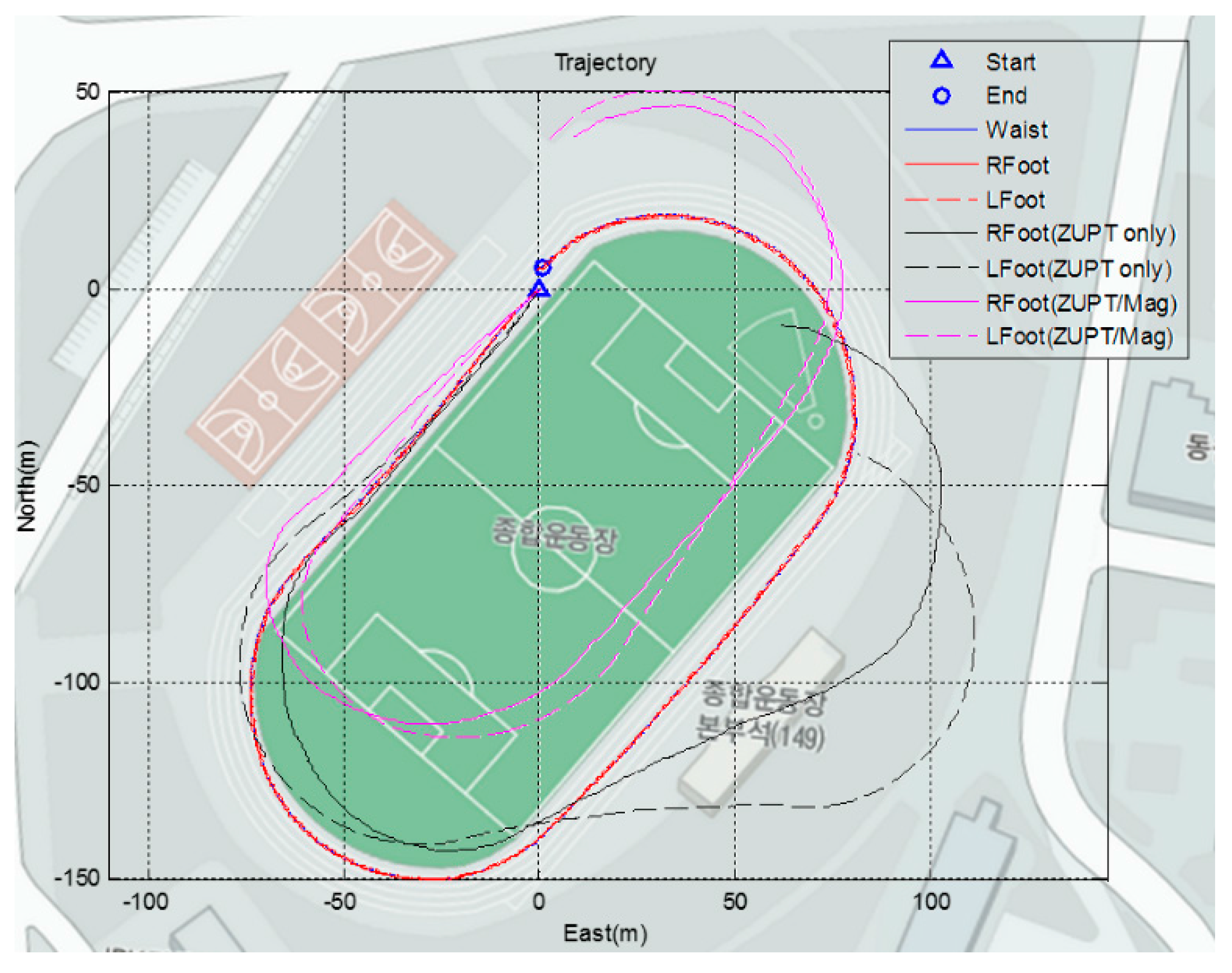

| ZUPT | Proposed Algorithm | ||||
|---|---|---|---|---|---|
| Right Foot | Left Foot | Right Foot | Left Foot | Waist | |
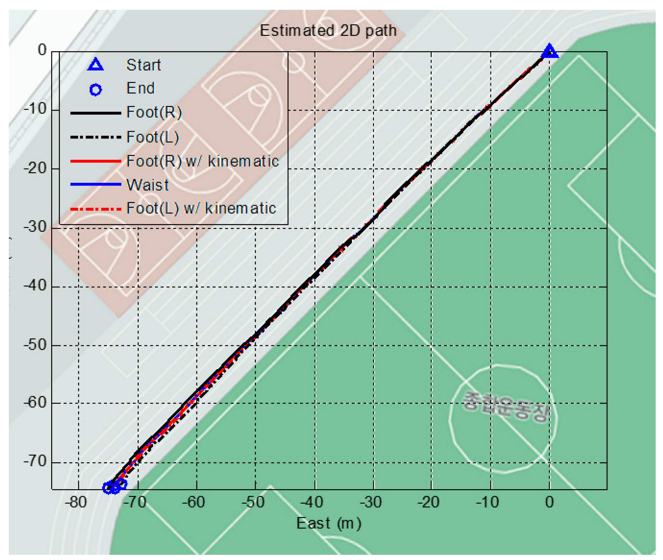
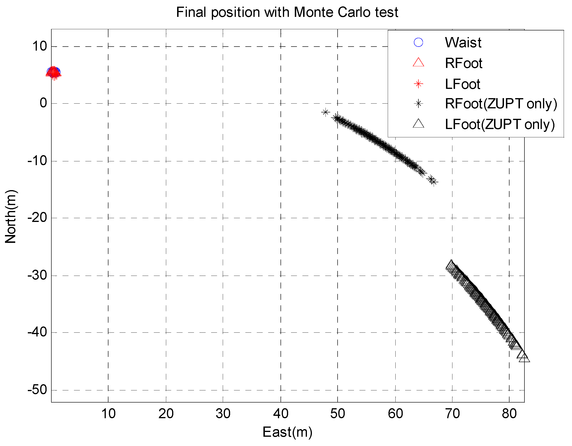
| RPE(m) | 57.3375 | 83.5120 | 5.4754 | 5.1073 | 5.5526 |
5. Conclusions
Acknowledgments
Author Contributions
Conflicts of Interest
References
- Lim, C.H.; Wan, Y. A Real-time indoor WiFi Localization System Utilizing Smart Antennas. IEEE Trans. Consum. Electron. 2007, 53, 618–622. [Google Scholar] [CrossRef]
- Kuban, D.A.; Dong, L.; Cheung, R.; Strom, E.; Crevoisier, R. Ultrasound-based Localization. Semina Radiat. Oncol. 2005, 15, 180–191. [Google Scholar] [CrossRef]
- Gezici, S.; Tian, Z.; Giannakis, G.B.; Kobayashi, H.; Molisch, A.F.; Poor, H.V.; Sahinoglu, Z. Localization via Ultra-wideband Radios: A Look at Positioning Aspects for Future Sensor Networks. IEEE Signal Proc. Mag. 2005, 22, 70–84. [Google Scholar] [CrossRef]
- Martin, E.; Vinyals, O.; Fiedland, G.; Bajcsy, R. Precise Indoor Localization Using Smartphones. In Proceedings of the International Conference on Multimedia, Firenze, Italy, 25–29 October 2010; pp. 787–790.
- Zou, H.; Jian, H.; Lu, X.; Xie, L. An Online Sequential Extreme Learning Machine Approach to WiFi Based Indoor Positioning. In Proceedings of the 2014 IEEE World Forum on the Internet of Things (WF-IoT), Seoul, Korea, 6–8 March 2014; pp. 111–116.
- Motion Capture Camera. Available online: www.vicon.com (accessed on 4 November 2015).
- Fritz, G.; Seifert, C.; Paletta, L. A Mobile Vision System for Urban Detection with Informative Local Descriptors. In Proceedings of the IEEE International Conference on Computer Vision Systems (ICVS’06), New York, NY, USA, 5–7 January 2006; p. 30.
- Lowe, D. Object Recognition from Local Scale-invariant Features. In Proceedings of the Seventh IEEE International Conference on Computer Vision, Kerkyra, Greece, 20–27 September 1999; Volume 2, pp. 1150–1157.
- Jirawimut, R.; Ptasinski, P.; Garaj, V.; Cecelja, F.; Balachandran, W. A Method for Dead Reckoning Parameter Correction in Pedestrian Navigation System. In Proceedings of the 18th IEEE Instrumentation and Measurement Technology Conference, Budapest, Hungary, 21–23 May 2001.
- Levi, R.W.; Judd, T. Dead Reckoning Navigational System using Accelerometer to Measure Foot Impacts. U.S. Patent 5,583,776, 10 December 1996. [Google Scholar]
- Ladetto, Q. On foot navigation: Continuous step calibration using both complementary recursive prediction and adaptive Kalman filtering. In Proceedings of the ION GPS 2000, Salt Lake City, UT, USA, 19–22 September 2000; pp. 1735–1740.
- Shin, S.H.; Park, C.G.; Hong, H.S.; Lee, J.M. MEMS-based Personal Navigator Equipped on the User’s Body. In Proceedings of the ION GNSS 2005, Long Beach, CA, USA, 13–16 September 2005.
- Kappi, J.; Syrjarinne, J.; Saarinen, J. MEMS-IMU Based Pedestrian Navigator for Handheld Devices. In Proceedings of the ION GPS 2001, Salt Lake City, UT, USA, 11–14 September 2001; pp. 1369–1373.
- Sagawa, K.; Susumago, M.; Inooka, H. Unrestricted Measurement Method of Three-dimensional Walking Distance Utilizing Body Acceleration and Terrestrial Magnetism. In Proceedings of the International Conference on Control, Automation and Systems, Jeju Island, Korea, 17 October 2001; pp. 707–710.
- Cho, S.Y.; Park, C.G.; Jee, G.I. Measurement System of Walking Distance using Low-Cost Accelerometers. In Proceedings of the 4th ASCC, Singapore, 25–27 September 2002.
- Gabaglio, V. Centralised Kalman Filter for Augmented GPS Pedestrian Navigation. In Proceedings of the ION GPS 2001, Salt Lake City, UT, USA, 11–14 September 2001; pp. 312–318.
- Aminian, K.; Jequier, E.; Schutz, Y. Level, Downhill and Uphill Walking Identification using Neural Networks. Electron. Lett. 1993, 29, 1563–1565. [Google Scholar] [CrossRef]
- Cho, S.Y. Design of a Pedestrian Navigation System and the Error Compensation Using RHKF Filter. Ph.D. Thesis, Kwangwoon University, Seoul, Korea, 2004. [Google Scholar]
- Cho, S.Y.; Park, C.G. A Calibration Technique for a Two-Axis Magnetic Compass in Telematics Devices. ETRI J. 2005, 27, 280–288. [Google Scholar] [CrossRef]
- Caruso, M.J.; Withanawasam, L.S. Vehicle Detection and Compass Applications Using AMR Magnetic Sensors. In Proceedings of Sensors Expo, Baltimore, MD, USA, 4–6 May 1999; pp. 477–489.
- White, C.E.; Bernstein, D.; Kornhauser, A.L. Some Map Matching Algorithms for Personal Navigation Assistants. Transp. Res. Part C Emerg. Technol. 2000, 8, 91–108. [Google Scholar] [CrossRef]
- Quddus, M.A. A General Map Matching Algorithm for Transport Telematics Applications. GPS Solut. 2003, 7, 157–167. [Google Scholar] [CrossRef] [Green Version]
- Ochieng, W.Y.; Quddus, M.A.; Noland, R.B. Integrated Positioning Algorithms for Transport Telematics Applications. In Proceedings of the ION Annual Conference, Dayton, OH, USA, 20–24 September 2004; pp. 692–705.
- Harle, R. A Survey of Indoor Inertial Positioning Systems for Pedestrians. IEEE Commun. Surv. Tutor. 2013, 15, 1281–1293. [Google Scholar] [CrossRef]
- Godha, S.; Lachapelle, G.; Cannon, M.E. Integrated GPS/INS system for pedestrian navigation in a signal degraded environment. In Proceedings of the 19th International Technical Meetings Satellite Division Institute Navigation, Fort Worth, TX, USA, 26–29 September 2006; pp. 2151–2164.
- Skog, I.; Handel, P.; Nilsson, J.-O.; Rantakokko, J. Zero-velocity detection—An algorithm evaluation. IEEE Trans. Biomed. Eng. 2010, 57, 2657–2666. [Google Scholar] [CrossRef] [PubMed]
- Cho, S.Y.; Park, C.G. MEMS based pedestrian navigation system. J. Navig. 2006, 59, 135–153. [Google Scholar] [CrossRef]
- Ascher, C.; Kessler, C.; Wankerl, M.; Trommer, G.F. Dual IMU indoor navigation with particle filter based map-matching on a smartphone. In Proceedings of the IEEE International Conference Indoor Positioning Indoor Navigation (IPIN), Zurich, Switzerland, 15–17 September 2010; pp. 1–5.
- Alvarez, J.C.; Alvarez, D.; López, A.; González, R.C. Pedestrian navigation based on a waist-worn inertial sensor. Sensors 2012, 12, 10536–10549. [Google Scholar] [CrossRef] [PubMed]
- Lan, K.-C.; Shih, W.-Y. Using simple harmonic motion to estimate walking distance for waist-mounted PDR. In Proceedings of the IEEE Wireless Communications and Networking Conference (WCNC), Paris, France, 14 April 2012; pp. 2445–2450.
- Mikov, A.; Moschevikin, A.; Fedorov, A.; Sikora, A. A localization system using inertial measurement units from wireless commercial handheld devices. In Proceedings of the IEEE International Conference Indoor Positioning Indoor Navigation (IPIN), Montbeliard, France, 28–31 October 2013; pp. 1–7.
- Liu, J.; Chen, R.; Pei, L.; Guinness, R.; Kuusniemi, H. A hybrid smartphone indoor positioning solution for mobile LBS. Sensors 2012, 12, 17208–17233. [Google Scholar] [CrossRef] [PubMed]
- Kothari, N.; Kannan, B.; Dias, M.B. Robust Indoor Localization on a Commercial Smart-Phone; Technical Report CMU-RI-TR-11–27; Carnegie-Mellon University: Pittsburgh, PA, USA, 2011. [Google Scholar]
- Lee, M.S.; Shin, S.H.; Park, C.G. Evaluation of a pedestrian walking status awareness algorithm for a pedestrian dead reckoning. In Proceedings of the ION GNSS 2010, Portland, OR, USA, 21–24 September 2010.
- Shin, S.H.; Lee, M.S.; Park, C.G. Pedestrian Dead Reckoning System with Phone Location Awareness Algorithm. In Proceedings of the PLANS 2010, Indian Wells, CA, USA, 4–6 May 2010.
- Saeedi, S.; Moussa, A.; El-Sheimy, N. Context-Aware Personal Navigation Using Embedded Sensor Fusion in Smartphones. Sensors 2014, 14, 5742–5767. [Google Scholar] [CrossRef] [PubMed]
- Masiero, A.; Guarnieri, A.; Pirotti, F.; Vettore, A. A Particle Filter for Smartphone-Based Indoor Pedestrian Navigation. Micromachines 2014, 5, 1012–1033. [Google Scholar] [CrossRef]
- Widyawan, P.G.; Munaretto, D.; Fischer, C.; An, C.; Lukowicz, P.; Klepal, M.; Timm-Giel, A.; Widmer, J.; Pesch, D.; Gellersen, H. Virtual lifeline: Multimodal sensor data fusion for robust navigation in unknown environments. Pervasive Mobile Comput. 2012, 8, 388–401. [Google Scholar] [CrossRef]
- Ju, H.J.; Lee, M.S.; Park, C.G. Advanced Heuristic Drift Elimination for Indoor Pedestrian Navigation. In Proceedings of the IPIN 2014, Busan, Korea, 27–30 October 2014.
- Rajagopal, S. Personal Dead Reckoning System with Shoe Mounted Inertial Sensors. Master’s Thesis, KTH Electrical Engineering, Stockholm, Sweden, 2008; pp. 1–45. [Google Scholar]
- Zampella, F.; Khider, M.; Robertson, P.; Jimenez, A. Unsented Kalman filter and Magnetic Angular Rate Update (MARU) for an improved Pedestrian Dead-Reckoning. In Proceedings of the IEEE Position Location and Navigation Symposium (PLANS), 2012 IEEE/ION, Myrtle Beach, SC, USA, 23–26 April 2012.
- Borenstein, J.; Lauro, O. Heuristic drift elimination for personnel tracking systems. J. Navig. 2010, 63, 591–606. [Google Scholar] [CrossRef]
- Roetenberg, D.; Luinge, H.; Slycke, P. Xsens MVN: Full 6DOF Human Motion Tracking Using Miniature Inertial Sensors. Available online: https://www.xsens.com/images/stories/PDF/MVN_white_paper.pdf (accessed on 4 November 2015).
- Yuan, Q.; Chen, I.-M.; Lee, S.P. SLAC:3D Localization of Human Based on Kinetic Human Movement Capture. In Proceedings of the 2011 IEEE International Conference on Robotic and Automation, Shanghai, China, 9–13 May 2011.
- Renaudin, V.; Yalak, K.; Tome, P. Hybridization of MEMS and Assisted GPS for Pedestrian Navigation. Inside GNSS 2007, January/February, 34–42. [Google Scholar]
- Jimenez, A.R.; Seco, F.; Prieo, J.C.; Guevara, J. Indoor Pedestrian Navigation using an INS/EKF framework for Yaw Drift Reduction and a Foot-mounted IMU. In Proceedings of the 7th Workshop on Positioning, Navigation and Communication, Dresden, Germany, 11–12 March 2010.
- Lee, M.S.; Ju, H.J.; Park, C.G. Step Length Estimation Algorithm for Firefighter using Linear Calibration. J. Inst. Control Robot. Syst. 2013, 19, 640–645. [Google Scholar] [CrossRef]
- Joo, H.J.; Lee, M.S.; Park, C.G. Stance Phase Detection Using Hidden Markov in Various Motions. In Proceedings of the IPIN 2013, Montbeliard, France, 28–31 October 2013.
© 2015 by the authors; licensee MDPI, Basel, Switzerland. This article is an open access article distributed under the terms and conditions of the Creative Commons Attribution license (http://creativecommons.org/licenses/by/4.0/).
Share and Cite
Lee, M.S.; Ju, H.; Song, J.W.; Park, C.G. Kinematic Model-Based Pedestrian Dead Reckoning for Heading Correction and Lower Body Motion Tracking. Sensors 2015, 15, 28129-28153. https://doi.org/10.3390/s151128129
Lee MS, Ju H, Song JW, Park CG. Kinematic Model-Based Pedestrian Dead Reckoning for Heading Correction and Lower Body Motion Tracking. Sensors. 2015; 15(11):28129-28153. https://doi.org/10.3390/s151128129
Chicago/Turabian StyleLee, Min Su, Hojin Ju, Jin Woo Song, and Chan Gook Park. 2015. "Kinematic Model-Based Pedestrian Dead Reckoning for Heading Correction and Lower Body Motion Tracking" Sensors 15, no. 11: 28129-28153. https://doi.org/10.3390/s151128129