
Comparative Analysis of GOCI Ocean Color Products

Abstract
:1. Introduction
2. Data

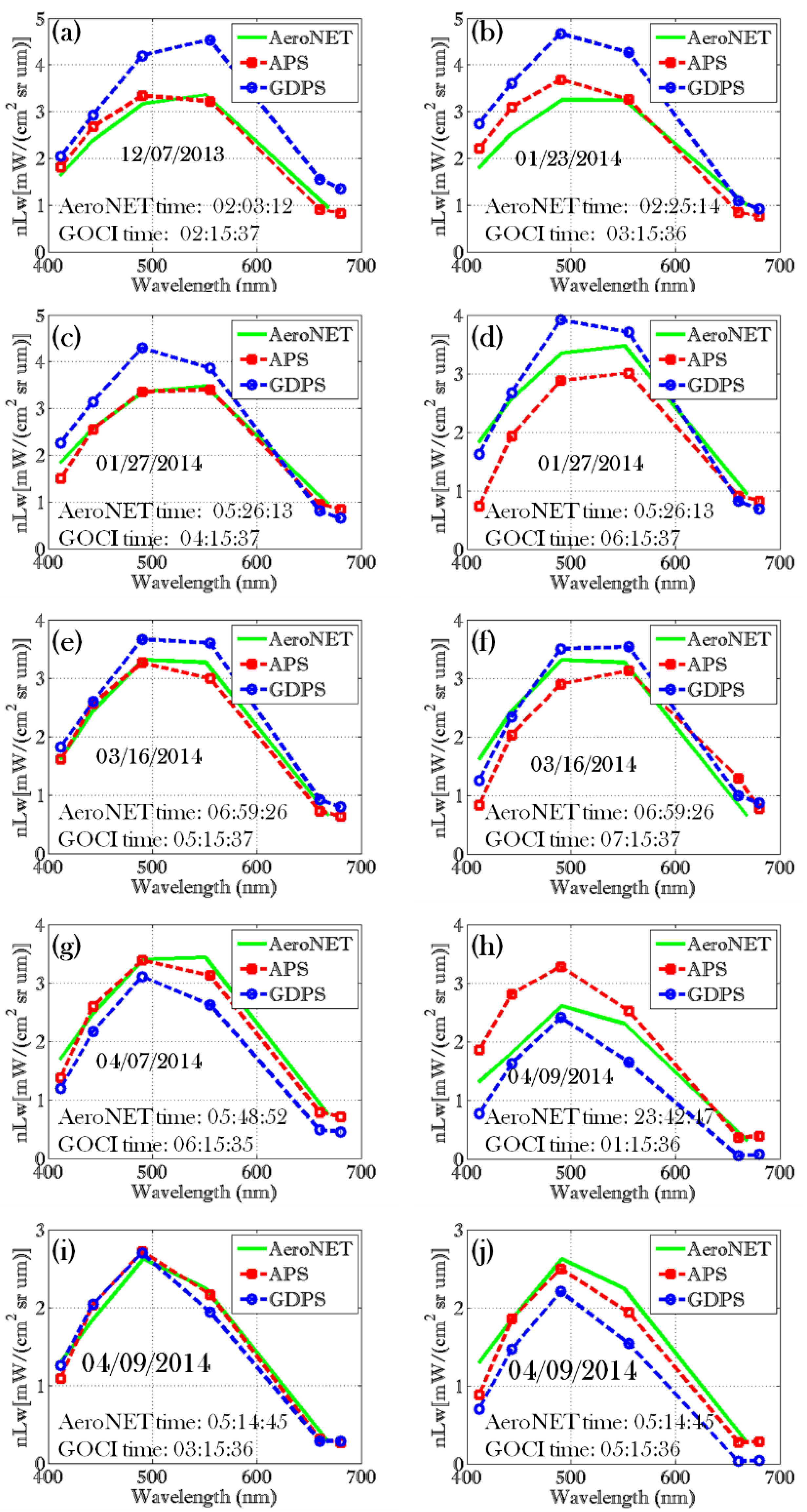
| Date | Time (GOCI) | Time (AeroNET) | Time Difference (in minute) |
|---|---|---|---|
| 12/07/2013 | 02:15:37 | 02:03:12 | 12 |
| 01/23/2014 | 03:15:36 | 02:25:14 | 50 |
| 01/27/2014 | 04:15:37 | 05:26:13 | 71 |
| 01/27/2014 | 06:15:37 | 05:26:13 | 49 |
| 03/16/2014 | 05:15:37 | 06:59:26 | 104 |
| 03/16/2014 | 07:15:37 | 06:59:26 | 16 |
| 04/07/2014 | 06:15:35 | 05:48:52 | 27 |
| 04/09/2014 | 01:15:36 | 23:42:47 * | 93 |
| 04/09/2014 | 03:15:36 | 05:14:45 | 119 |
| 04/09/2014 | 05:15:36 | 05:14:45 | 01 |
3. Results and Discussion
3.1. AeroNET vs. Satellite
| AeroNET vs. APS vs. GDPS | ||||
|---|---|---|---|---|
| AeroNET vs. APS | ||||
| RMSE | 0.52 | 0.46 | 0.33 | 0.24 |
| APD | 26.84% | 15.86% | 8.23% | 6.79% |
| AeroNET vs. GDPS | ||||
| RMSE | 0.49 | 0.47 | 0.69 | 0.67 |
| APD | 26.72% | 15.91% | 17.24% | 19.92% |
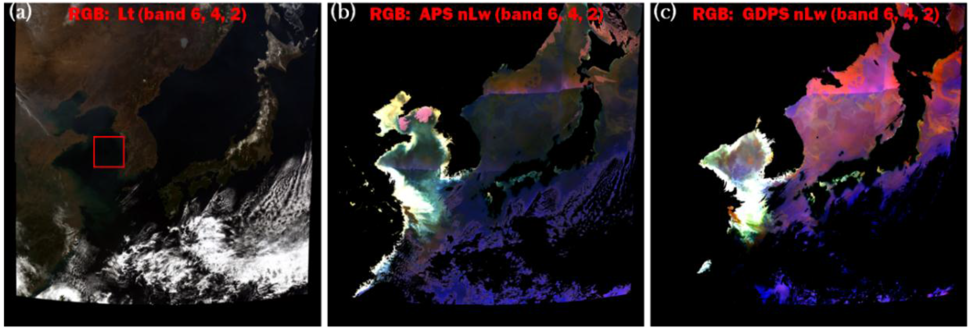
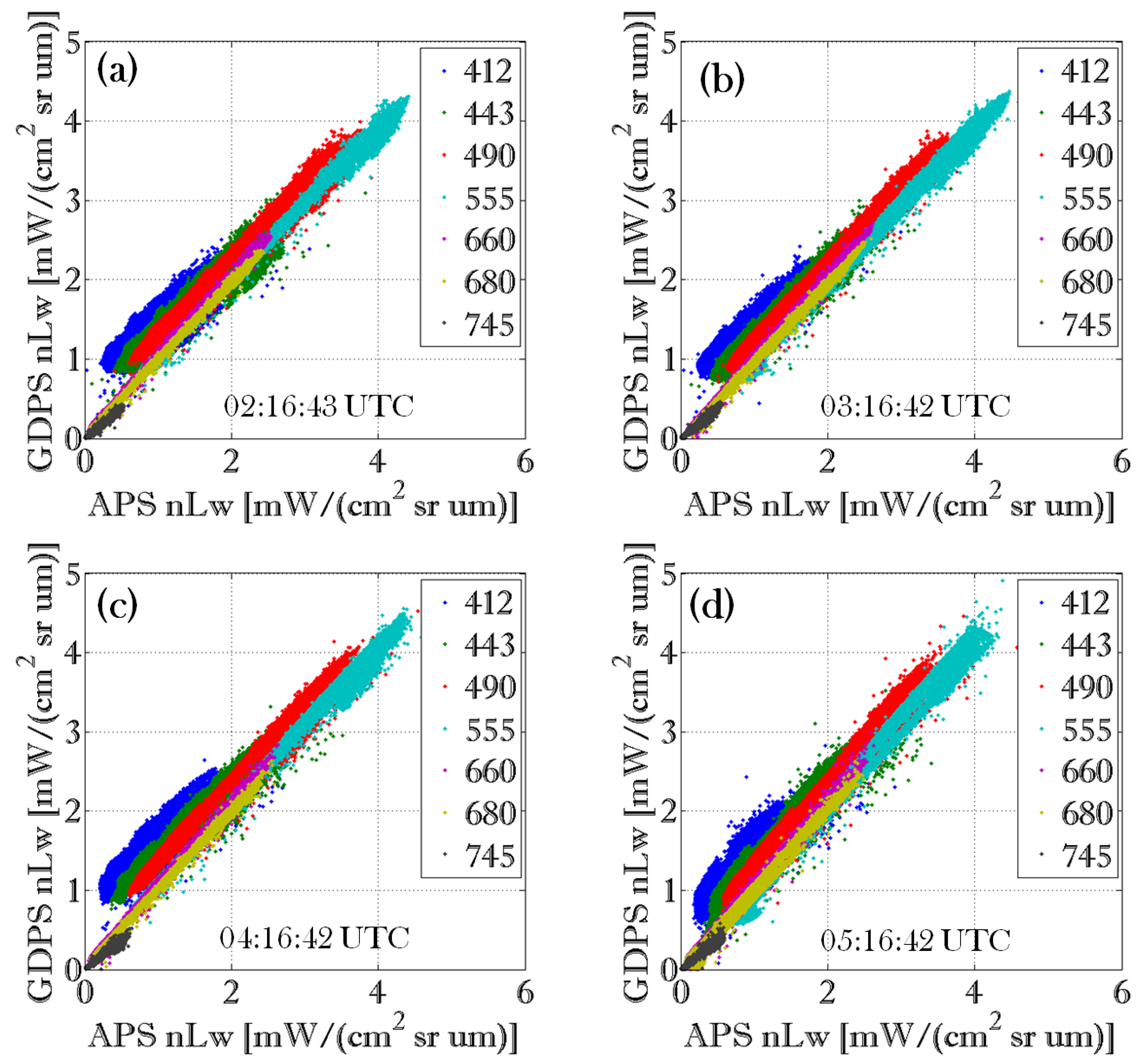
3.2. APS vs. GDPS Results
| Acquisition Time | # of Valid Pixels APS | # of Valid Pixels GDPS | # of Valid | |||||||
|---|---|---|---|---|---|---|---|---|---|---|
| 02:16 UTC | 228,015 (2.83% more valid pixels) | 221,495 | 221,492 | r2 = 0.84 | r2 = 0.95 | r2 = 0.99 | r2 = 0.99 | r2 = 0.99 | r2 = 0.99 | r2 = 0.99 |
| S = 0.72 | S = 0.85 | S = 0.94 | S = 0.96 | S = 1.00 | S = 0.97 | S = 0.75 | ||||
| I = 0.75 | I = 0.50 | I = 0.37 | I = 0.07 | I = 0.04 | I = 0.02 | I = 0.00 | ||||
| 03:16 UTC | 228,541 (2.10% more valid pixels) | 223,709 | 223,708 | r2 = 0.91 | r2 = 0.97 | r2 = 0.99 | r 2 = 0.99 | r2 = 0.99 | r2 = 0.99 | r2 = 0.99 |
| S = 0.80 | S = 0.91 | S = 0.99 | S = 0.99 | S = 1.04 | S = 1.00 | S = 0.77 | ||||
| I = 0.67 | I = 0.39 | I = 0.24 | I = −0.02 | I = -0.02 | I = −0.04 | I = −0.01 | ||||
| 04:16 UTC | 228,936 (2.00% more valid pixels) | 224,338 | 224,337 | r2 = 0.92 | r2 = 0.98 | r2 = 0.99 | r2 = 0.99 | r2 = 0.99 | r2 = 0.99 | r2 = 0.99 |
| S = 0.84 | S = 0.93 | S = 1.00 | S = 1.01 | S = 1.04 | S = 1.00 | S = 0.75 | ||||
| I = 0.84 | I = 0.57 | I = 0.39 | I = 0.08 | I = 0.05 | I = 0.03 | I = 0.00 | ||||
| 05:16 UTC | 229,027 (5.93% more valid pixels) | 215,369 | 215,368 | r2 = 0.86 | r2 = 0.96 | r2 = 0.98 | r2 = 0.99 | r2 = 0.97 | r2 = 0.97 | r2 = 0.96 |
| S = 1.10 | S = 1.09 | S = 1.11 | S = 1.09 | S = 1.10 | S = 1.05 | S =0 .76 | ||||
| I = 0.54 | I = 0.28 | I = 0.14 | I = −0.08 | I = −0.02 | I = −0.03 | I = −0.01 |
4. Conclusions
Acknowledgments
Author Contributions
Conflicts of Interest
References
- Choi, J.K.; Park, Y.J.; Ahn, J.H.; Lim, H.-S.; Eom, J.; Ryu, J.-H. GOCI, the world’s first geostationary ocean color observation satellite, for the monitoring of temporal variability in coastal water turbidity. J. Geophys. Res. 2012, 117. [Google Scholar] [CrossRef]
- Ryu, J.-H.; Han, H.-J.; Cho, S.; Park, Y.J.; Ahn, Y.H. Overview of Geostationary Ocean Color Imager (GOCI) and GOCI dataprocessing system (GDPS). Ocean Sci. J. 2012, 47, 223–233. [Google Scholar] [CrossRef]
- Amin, R.; Zhou, J.; Gilerson, A.; Gross, B.; Moshary, F.; Ahmed, S. Novel Optical Techniques for Detecting and Classifying Toxic Dinoflagellate Karenia Brevis Blooms Using Satellite Imagery. Opt. Express 2009, 17, 9126–9144. [Google Scholar] [CrossRef] [PubMed]
- Amin, R.; Gilerson, A.; Gross, B.; Moshary, F.; Ahmed, S. MODIS and MERIS detection of dinoflagellates blooms using the RBD technique. In Proceedings of the Remote Sensing of the Ocean, Sea Ice, and Large Water Regions 2009, Berlin, Germany, 31 August–3 September 2009.
- Belward, A.S.; Valenzuela, C.R. Remote Sensing and Geographical Information System for Resource Management in Developing Countries; Kluwer Academic: Dordrecht, the Netherlands, 1991. [Google Scholar]
- Amin, R.; Gould, R.; Hou, W.; Arnone, R.; Lee, Z.P. Optical algorithm for cloud shadow detection over water. IEEE Trans. Geosci. Remote Sens. 2013, 51, 732–741. [Google Scholar] [CrossRef]
- Amin, R.; Lewis, D.; Gould, R.W.; Hou, W.; Lawson, A.; Ondrusek, M.; Arnone, R. Assessing the application of cloud shadow atmospheric correction algorithm on HICO. IEEE Trans. Geosci. Remote Sens. 2014, 52, 2646–2653. [Google Scholar] [CrossRef]
- Amin, R.; Penta, B.; Derada, S. Occurrence and spatial extent of HABs on the West Florida Shelf 2002-present. IEEE Geosci. Remote Sens. Lett. 2015, 12, 2080–2084. [Google Scholar] [CrossRef]
- Amin, R.; Shulman, I. Hourly Turbidity Monitoring Using Geostationary Ocean Color Imager Fluorescence Bands. J. Appl. Remote Sens. 2015, 9. [Google Scholar] [CrossRef]
- Yamaguchi, Y.; Kahle, A.B.; Tsu, H.; Kawakami, T.; Pniel, M. Overview of Advanced Spaceborne Thermal Emission and Reflection Radiometer (ASTER). IEEE Trans. Geosci. Remote Sens. 1998, 36, 1062–1071. [Google Scholar] [CrossRef]
- Justice, C.O.; Townshend, J.R.G.; Vermote, E.F.; Masuoka, E.; Wolfe, R.E.; Saleous, N.; Roy, D.P.; Morisette, J.T. An Overview of MODIS Land Data Processing and Product Status. Remote Sens. Environ. 2002, 83, 3–15. [Google Scholar] [CrossRef]
- Gordon, H.R.; Du, T.; Zhang, T. Remote sensing of ocean color and aerosol properties: Resolving the issue of aerosol absorption. Appl. Opt. 1997, 36, 8670–8684. [Google Scholar] [CrossRef]
- Amin, R.; Gilerson, A.; Zhou, J.; Gross, B.; Moshary, F.; Ahmed, S. Impacts of atmospheric corrections on algal bloom detection techniques. In Proceedings of the Eighth Conference on Coastal Atmospheric and Oceanic Prediction and Processes, Phoenix, AZ, USA, 10–15 January 2009.
- Martinolich, P.; Scardino, T. Automated Processing System User’s Guide Version 4.2. Avaliable online: http://www7333.nrlssc.navy.mil/docs/aps_v4.2/html/user/aps_chunk/index.xhtml (accessed on 7 June 2015).
- Han, H.J.; Ryu, J.H.; Ahn, Y.H. Development of Geostationary Ocean Color Imager (GOCI) Data Processing System (GDPS). Korean Soc. Remote Sens. 2010, 26, 239–249. [Google Scholar]
- Yang, H.; Oh, E.; Han, T.H.; Han, H.J.; Choi, J.K. An Efficient Data Processing Method to Improve the Geostationary Ocean Color Imager (GOCI) Data Service. Korean J. Remote Sens. 2014, 30. [Google Scholar] [CrossRef]
- Han, H.J.; Ryu, J.H.; Cho, S.; Yang, C.S.; Ahn, Y.H. Preliminary verification results of the geostationary ocean color satellite data processing software system. In Proceedings of the Geostationary Ocean Color Imager (GOCI) Technical Development, Operation, and Applications, Incheon, Korea, 11 October 2010.
- Zibordi, G.; Mélin, F.; Berthon, J.-F. AERONET-OC: A Network for the Validation of Ocean Color Primary Products. J. Atmos. Ocean Technol. 2009, 26, 1634–1651. [Google Scholar] [CrossRef]
- Clark, D.K.; Feinholz, M.; Yarbrough, M.; Johnson, B.C.; Brown, S.W.; Kim, Y.S.; Barnes, R.A. Overview of the Radiometric Calibration of MOBY. In Proceedings of the Earth Observing Systems VI, San Diego, CA, USA, 29 July 2001.
- Lawson, A.; Arnone, R.A.; Gould, R.W.; Scardino, T.L.; Martinolich, P.M.; Ladner, S.W.; Lewis, M.D. Comparison of Long Island Sound and Martha’s Vineyard Waters. In Proceedings of the NASA A-Train Meeting, New Orleans, LA, USA, 25–28 October 2010.
- Lawson, A.; Arnone, R.; Gould, R.; Scardino, T.; Martinolich, P.M.; Ladner, S.; Lewis, D. Automated System to Facilitate Vicarious Calibration of Ocean Color Systems. In Proceedings of the Mississippi Water Resources Conference, Bay St. Louis, MS, USA, 3–5 November 2010.
- Lewis, M.D.; Amin, R.; Gallegos, S.; Gould, R.W., Jr.; Ladner, S.; Lawson, A.; Li, R. Improving remotely sensed fused ocean data products through cross-sensor calibration. J. Appl. Remote Sens. 2015, 9. [Google Scholar] [CrossRef]
- Franz, B.A.; Bailey, S.W.; Werdell, P.J.; McClain, C.R. Sensor independent approach to the vicarious calibration of satellite ocean color radiometry. Appl. Opt. 2007, 46, 5068–5082. [Google Scholar] [CrossRef] [PubMed]
- Bailey, S.W.; Hooker, S.B.; Antoine, D.; Franz, B.A.; Werdell, P.J. Sources and assumptions for the vicarious calibration of ocean color satellite observations. Appl. Opt. 2008, 47, 2035–2045. [Google Scholar] [CrossRef] [PubMed]
- Ocean Color. Avaliable online: http://Oceancolor.Gsfc.Nasa.Gov/Cms/ (accessed on 6 July 2015).
- Crout, R.L.; Ladner, S.; Amin, R.; Lawson, A.; Arnone, R.A. Evaluation of GOCI, MODIS and VIIRS. In Proceedings of the Ocean Sciences Meeting, Honolulu, HI, USA, 23–28 February 2014.
- Gordon, H.R.; Wang, M. Retrieval of water-leaving radiance and aerosol optical thickness over the oceans with SeaWiFS: A preliminary algorithm. Appl. Opt. 1994, 33, 443–452. [Google Scholar] [CrossRef] [PubMed]
- Lamquin, N.; Mazeran, C.; Doxaran, D.; Ryu, J.H.; Park, Y.J. Assessment of GOCI radiometric products using MERIS, MODIS and field measurements. Ocean Sci. J. 2012, 47, 287–311. [Google Scholar] [CrossRef]
© 2015 by the authors; licensee MDPI, Basel, Switzerland. This article is an open access article distributed under the terms and conditions of the Creative Commons Attribution license (http://creativecommons.org/licenses/by/4.0/).
Share and Cite
Amin, R.; Lewis, M.D.; Lawson, A.; Gould Jr., R.W.; Martinolich, P.; Li, R.-R.; Ladner, S.; Gallegos, S. Comparative Analysis of GOCI Ocean Color Products. Sensors 2015, 15, 25703-25715. https://doi.org/10.3390/s151025703
Amin R, Lewis MD, Lawson A, Gould Jr. RW, Martinolich P, Li R-R, Ladner S, Gallegos S. Comparative Analysis of GOCI Ocean Color Products. Sensors. 2015; 15(10):25703-25715. https://doi.org/10.3390/s151025703
Chicago/Turabian StyleAmin, Ruhul, Mark David Lewis, Adam Lawson, Richard W. Gould Jr., Paul Martinolich, Rong-Rong Li, Sherwin Ladner, and Sonia Gallegos. 2015. "Comparative Analysis of GOCI Ocean Color Products" Sensors 15, no. 10: 25703-25715. https://doi.org/10.3390/s151025703
APA StyleAmin, R., Lewis, M. D., Lawson, A., Gould Jr., R. W., Martinolich, P., Li, R.-R., Ladner, S., & Gallegos, S. (2015). Comparative Analysis of GOCI Ocean Color Products. Sensors, 15(10), 25703-25715. https://doi.org/10.3390/s151025703