BeiDou Inter-Satellite-Type Bias Evaluation and Calibration for Mixed Receiver Attitude Determination


Abstract
: The Chinese BeiDou system (BDS), having different types of satellites, is an important addition to the ever growing system of Global Navigation Satellite Systems (GNSS). It consists of Geostationary Earth Orbit (GEO) satellites, Inclined Geosynchronous Satellite Orbit (IGSO) satellites and Medium Earth Orbit (MEO) satellites. This paper investigates the receiver-dependent bias between these satellite types, for which we coined the name “inter-satellite-type bias” (ISTB), and its impact on mixed receiver attitude determination. Assuming different receiver types may have different delays/biases for different satellite types, we model the differential ISTBs among three BeiDou satellite types and investigate their existence and their impact on mixed receiver attitude determination. Our analyses using the real data sets from Curtin's GNSS array consisting of different types of BeiDou enabled receivers and series of zero-baseline experiments with BeiDou-enabled receivers reveal the existence of non-zero ISTBs between different BeiDou satellite types. We then analyse the impact of these biases on BeiDou-only attitude determination using the constrained (C-)LAMBDA method, which exploits the knowledge of baseline length. Results demonstrate that these biases could seriously affect the integer ambiguity resolution for attitude determination using mixed receiver types and that a priori correction of these biases will dramatically improve the success rate.1. Introduction
The Chinese BeiDou System (BDS), having different types of satellites, is an important addition to the ever growing system of Global Navigation Satellite Systems (GNSS). The BDS currently under development will consist of five Geostationary Earth Orbit (GEO) satellites, three Inclined Geosynchronous Satellite Orbit (IGSO) satellites and twenty-seven Medium Earth Orbit (MEO) satellites [1,2]. Presently, it consists of five GEO, five IGSO and four MEO satellites transmitting navigation signals in quadrature phase-shift keying (QPSK) modulation on a total of three frequency bands (B1, B2, B3). This paper investigates the receiver-dependent bias between these satellite types, for which we coined the name “inter-satellite-type bias” (ISTB), and its impact on mixed receiver attitude determination.
Having 14 fully operational satellites, BDS has already had the standalone capability of satellite-based positioning, navigation and timing (PNT) solutions, at least in the Asia-Pacific region. Analyses of BeiDou-based PNT solutions have been reported in various studies. Apart from simulation-based studies in [3–7], analyses of BeiDou PNT with real data have been reported in [8–18]. Measurement quality and relative positioning analyses with real data collected using Chinese GNSS receivers (UB240-CORS) are reported in [10,19]. Precise point positioning results with the same receiver type are reported in [15]. Initial assessment of real data collected using non-Chinese GNSS receivers and with post-processed orbit and clock products [20,21] independent of the control segment is reported in [8]. The same products are used to analyse precise point positioning in [11,14] and triple-frequency relative positioning in [9]. Similar products are used in [12] to analyse the contribution of BeiDou in single point positioning. With the recent release of BeiDou interface control document (ICD) [1], one can expect increased research on BeiDou based-PNT solutions outside China.
Multiple GNSS receivers/antennas rigidly mounted on a platform can be used to determine platform attitude (orientation) (see, for example [22–28]). GNSS-based attitude determination offers several advantages, including that it is not affected by drift, is lower in cost and requires less maintenance than traditional methods. Precise attitude determination, however, relies on successful resolution of the integer carrier phase ambiguities. The least squares ambiguity decorrelation adjustment (LAMBDA) method [29] is currently the standard method for solving unconstrained and linearly-constrained GNSS ambiguity resolution problems (see, for example [30–37]). For such models, the method is known to be numerically efficient and optimal in the sense that it provides integer ambiguity solutions with the highest possible success-rate [38–40]. To exploit the known baseline length, we make use of the constrained (C-)LAMBDA method [41–49]. BeiDou-based attitude determination using identical receivers has been analysed in [16–18].
In this paper, we consider mixed receiver attitude determination using single- and dual-frequency BeiDou observables. Assuming different receiver types may have different delays/biases for different satellite types, we model the differential ISTBs among three BeiDou satellite types. We develop an extended GNSS model, taking into account these biases, and describe the estimation of these biases. Our analyses using the data from two real data campaigns (one is with Curtin's permanent GNSS array consisting of different types of BeiDou-enabled receivers, and the other is with zero-baseline using BeiDou enabled receivers) reveal the existence of non-zero ISTBs between different BeiDou satellite types. We observe that these biases are stable and constant. Hence, we use a priori estimated biases to correct BeiDou observations, so that one can use classical double difference processing without loosing redundancy. We then analyse the impact of these biases on BeiDou-only attitude determination using the constrained (C-)LAMBDA method, which exploits the knowledge of baseline length. Results demonstrate that ISTBs could seriously affect the integer ambiguity resolution for attitude determination using mixed receiver types and that a priori correction of these biases will dramatically improve the success rate.
This contribution is organized as follows. Section 2 describes the functional and stochastic model for BeiDou observations, with special attention to ISTBs and associated processing approaches. Section 3 formulates the quadratically-constrained BeiDou model for attitude determination and describes the C-LAMBDA method. Section 4 demonstrates the existence of non-zero ISTBs between different BeiDou satellite types using real data and presents the results of attitude determination, revealing the impact of ISTBs. Finally, Section 5 contains the summary and conclusions of this contribution.
2. BeiDou Observations
This section presents the BeiDou observation model, distinguishing satellite types, namely GEO, IGSO and MEO, to accommodate receiver-dependent delays (biases) for different satellite types. Since the BeiDou system uses the code division multiple access (CDMA) technique, the code and phase observations of receiver r tracking satellite sβ of type β at frequency j, denoted by and , respectively, are given as [50]:
The between-receiver single difference (SD) pseudo-range and carrier-phase observations of two BeiDou receivers, r and 1, at frequency j from satellite sβ of type β, denoted as and , respectively, are given as:
Further differencing the above SD observables between satellites eliminates the receiver-dependent biases: with the first satellite of the satellite-type 1 as the pivot, the double difference (DD) observables are given as:
In classical double differencing for single satellite-type systems, such as GPS, the terms, and do not exist. However, as shown in Section 4.2, there may exist non-zero differential inter-satellite-type biases (ISTBs) for the BeiDou system if one uses mixed receiver types. That is, and for β ≠ 1.
The linearized DD observation equations corresponding to Equations (5) and (6) read:
The vectorial forms of the DD observation equations for the jth frequency read:
When combining the single-epoch, multi-frequency linearized DD GNSS code and phase observation Equations (9) and (10), we obtain the mixed integer model of observation equations:
2.1. Classical DD Model
The naive approach is to simply ignore the third term in Equation (18), resulting in the classical baseline model with a full-rank system:
2.2. Extended DD Model with Estimable ISTBs
The rank deficiency in Equation (18) can be removed by constraining a set of parameters (combinations) as the S-basis [53-55]. The number of S-basis constraints equals the size of the rank deficiency There are many possibilities to choose S-basis constraints. One such choice corresponds to a reparametrization in Equation (6), such that the DD ambiguities of the pivot satellites of second satellite types are combined with corresponding phase ISTBs:
Another option, i.e., another S-basis choice, is to lump the phase ISTB with the average of two or more DD ambiguities of the second satellite type. For example, if we lump the phase ISTB with the average of all DD ambiguities of the second satellite type, the DD phase observations of the second satellite type read:
For this choice of S-basis, however, the fractional part of the estimable phase ISTB is not necessarily equal to that of the actual phase ISTB. Having different choices, one should be cautious while interpreting or using the estimated phase ISTBs based on a given S-basis choice.
In this contribution, we consider the parametrization of Equations (20) and (21), which has the simple interpretation that the estimable integer ambiguities correspond to satellite type-specific double differencing (see Section 2.3), and moreover, it enables us to observe the fractional parts of the phase ISTBs (see Section 4.2). For our choice of S-basis, the full-rank (extended) model reads:
2.3. Type-Specific DD Model
Since ISTBs are nuisance parameters, one can eliminate 2f(η− 1) ISTBs using the differencing operator,
 = I2 ⊗ If ⊗ blockdiag
, in which
is the differencing matrix. Pre-multiplying Equation (26) by
nullifies the third term and results in a type-specific DD model, which has a reference satellite (pivot) per satellite type and reads:
= I2 ⊗ If ⊗ blockdiag
, in which
is the differencing matrix. Pre-multiplying Equation (26) by
nullifies the third term and results in a type-specific DD model, which has a reference satellite (pivot) per satellite type and reads:
y the 2f(m − η) × 1 vector of type-specific DD observations, A̿=
Ā = [L̿T, 0T]T is the 2f(m − η) × f(m − η) design matrix with f(m −η) × f(m − η) matrix L̿ = diag(λ1,…, λf) ⊗ blockdiag (Im1−1, Im2−1,…, Imη−1) and Ḡ =
G is the 2f(m − η) × 3 geometry matrix. This model has 2f(η −1) less observations and 2f(η − 1) less unknown parameters than Equation (26). Hence, both models have the same redundancy and are equivalent.2.4. ISTB-Corrected DD Model
As shown in Section 4.2, ISTBs are stable and can be assumed to be constant for a given receiver type pair. Hence, one can correct DD observations in Equation (18) with a priori estimates of ISTBs (calibration):
Finally, Table 1 summarizes the full-rank models described in the above. For further analyses in this paper, we only consider three models, namely, the classical DD model, ignoring ISTBs, the extended model and the classical DD model with ISTB correction. The type-specific DD model is equivalent to the extended DD model.
2.5. Stochastic Model
We assume elevation-dependent noise characteristics [56] for the undifferenced observables in Equations (1) and (2). That is, the standard deviation of the undifferenced observable, ς, can be written as:
To construct the stochastic model for the observations in Equation (18), consider the undifferenced observations reading:
For type-specific DD observations in Equation (27), the dispersion matrix is given as:
3. BeiDou Attitude Determination
Since attitude determination uses rigidly mounted antennas, the baseline length is a priori known and can be used to strengthen the underlying model. With the inclusion of the baseline length constraint to the models in Equations (19), (26) or (28) and with the stochastic model in Equation (34), we obtain the GNSS compass model [42,47]:
| Classical model Equation (19): | y= y, |  = A = A | z= z, | = [ ], | h = [ ], | κ = f(m−1) |
| Extended model Equation (26): | y = y, | = Ā | z = z̄, | =H, | h = h̄, | κ = f(m− η) |
| ISTBcorrected classical model Equation (28): | y = ỹ, | = A | z = z, | = [ ], | h= [ ], | κ = f(m−1) |
In the above, the baseline is constrained to lie on a sphere with radius l (
 = {b ∈ ℝ3 | ‖b‖ = l}). Our objective is to solve for b in a least-squares sense, thereby taking the integer constraints on z and the quadratic constraint on vector b into account. Hence, the least-squares minimization problem that will be solved reads:
3.1. The Ambiguity Resolved Attitude
We now describe the steps for computing the integer ambiguity resolved attitude angles.
3.1.1. The Real-Valued Float Solution
The float solution is defined as the solution of Equation (39) without the constraints. When we ignore the integer constraints on z and the quadratic constraint on b, the float solutions, ẑ, b̂ and ĥ, and their variance-covariance matrices are obtained as follows:
Using the above estimates, the original problem in Equation (39) can be decomposed as:
3.1.2. The Integer Ambiguity Resolution
Based on the orthogonal decomposition Equation (46), the quadratic-constrained integer minimiza-tion can be formulated as:
, in the metric of Qb̂(z)b̂(z).Unlike with the standard LAMBDA method [29], the search space of the above minimization problem is non-ellipsoidal, due to the presence of the second term in the ambiguity objective function. Moreover, its solution requires the computation of a nonlinear-constrained least-squares problem (49) for every integer vector in the search space. In the C-LAMBDA method, this problem is mitigated through the use of easy-to-evaluate bounding functions [47]. Using these bounding functions, two strategies, namely the Expansion and the Search and Shrink strategies, were developed; see, e.g., [41,45]. These techniques avoid the computation of Equation (49) for every integer vector in the search space and compute the integer minimizer, ẑ, in an efficient manner.
3.1.3. The Ambiguity Resolved Parameter Estimation
For a single baseline, b is related to the Euler-angles, ξ = [Φ, θ]T, with Φ the heading and θ the elevation, as b(ξ) = lu(ξ), where u(ξ) = [cθcΦ, cθsΦ, −sθ]T, with sα = sin(α) and cα = cos(α). The sought for attitude angles, ξ (ž), are the reparametrized solution of Equation (49). Using a first order approximation, the formal variance-covariance matrix of the ambiguity resolved, estimated heading and elevation angles are given by:
4. Analyses
4.1. Measurement Campaign
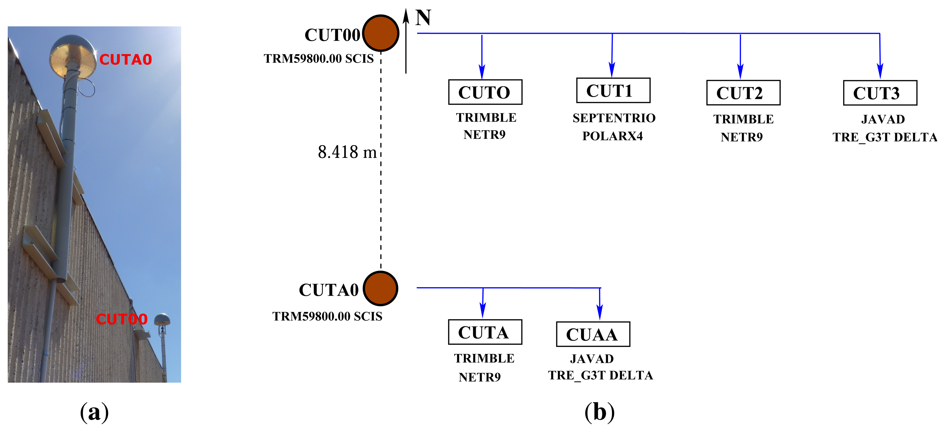
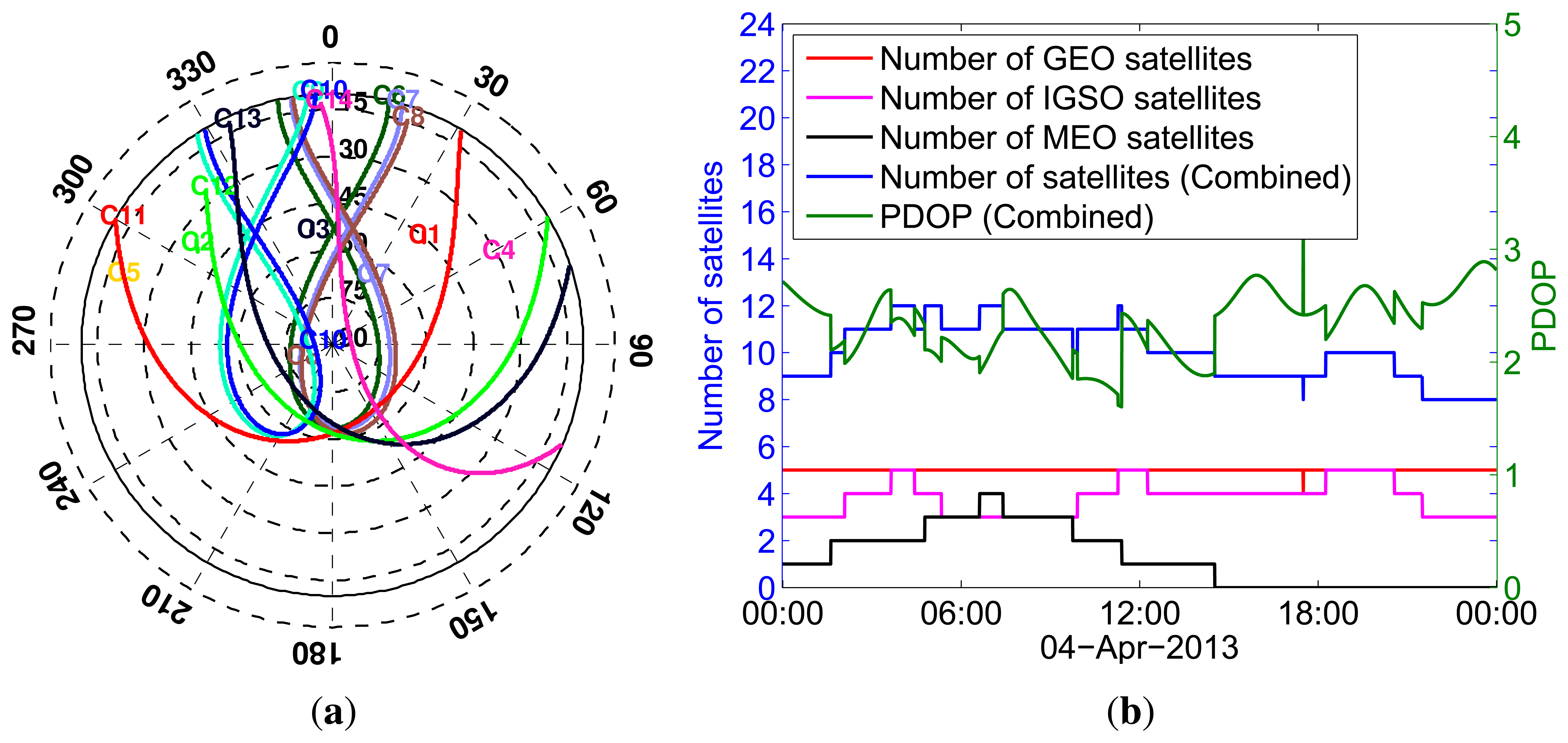
The analyses in this paper are based on data sets from Curtin University's permanent GNSS stations and series of zero-baseline experiments. The first data set is from Curtin's permanent GNSS antennas (CUT00 and CUTA0) mounted on the roof of building 402 at the campus of Curtin University in Perth, Australia (Figure 1a). These antennas are connected to six BeiDou-enabled receivers, as summarised in Figure 1b, consisting of three Trimble NETR9, two Javad TRE_G3T DELTA and a Septentrio POLARx4 receivers. We considered the data from these receivers for five days from April 4 to 8, 2013. BeiDou satellite visibility for April 4 is shown in Figure 2. The data of various zero baselines for five days with a 30 s sampling interval is used to estimate ISTBs in Section 4.2, while the data of various short baselines between CUT00 and CUTA0 on April 7 with a 1 s sampling interval is used to analyse the impact of ISTBs on attitude determination in Section 4.3.
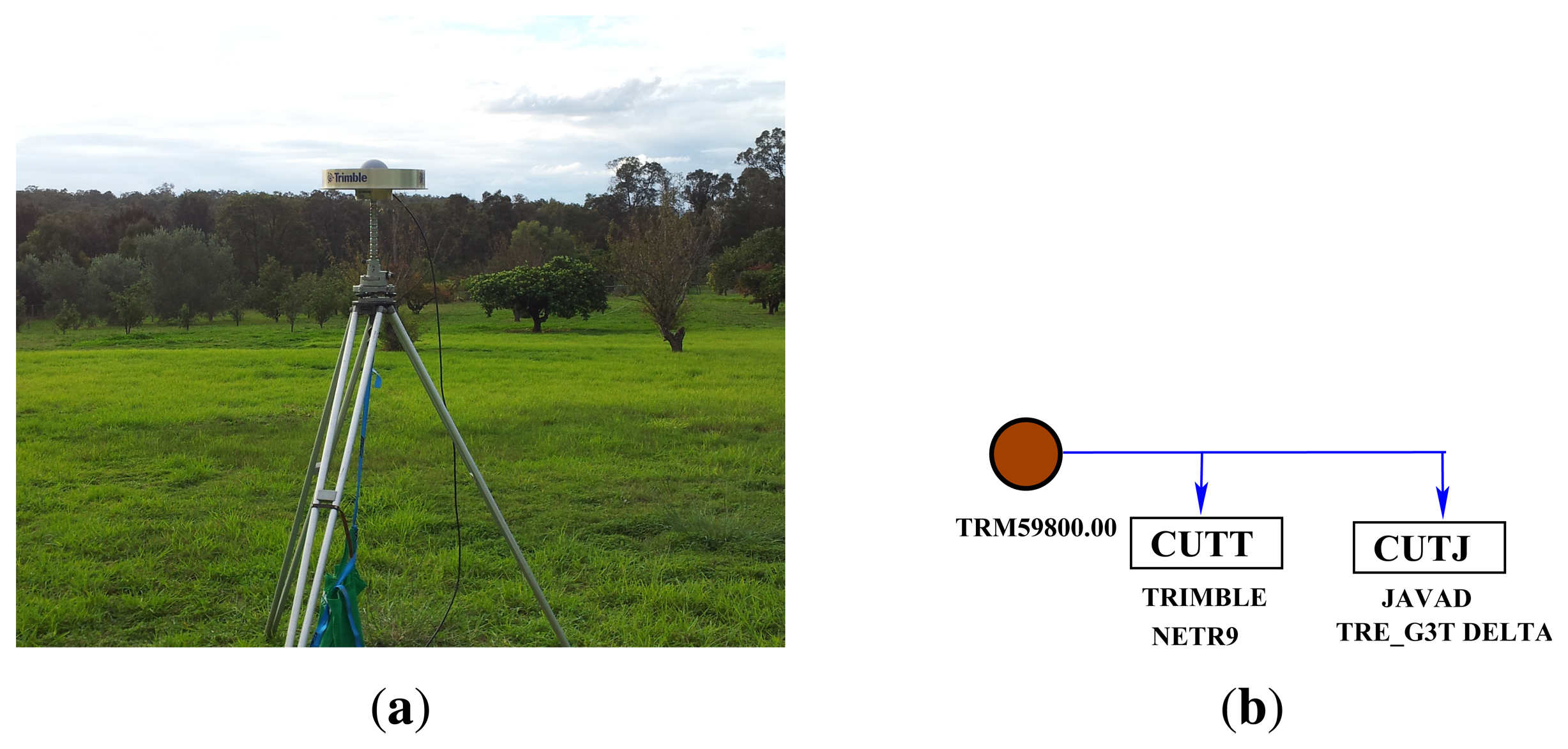
In addition to the data from Curtin's permanent stations, we also carried out a series of zero-baseline experiments: two in an open space in Curtin University and another two in an open space in Kalamunda, Western Australia (about 17 km from Curtin University), each for three consecutive days (Table 2). As shown in Figure 3b, a single antenna (Figure 3a) was connected to two BeiDou-enabled receivers (Trimble NETR9 and Javad Javad TRE G3T DELTA). Figure 4 shows the visibility of BeiDou satellites on April 19, 2013. These zero-baseline data sets (with a 30 s sampling interval) are also used to estimate and validate ISTBs in Section 4.2. The stochastic model parameters of the elevation-dependent model Equation (29) for the receivers are reported in Table 3. Since the receivers, except Trimble NETR9, track only B1 and B2 signals, single- and dual-frequency analyses are considered in the paper.
4.2. BeiDou Inter-Satellite-Type Bias (ISTB)
First, we considered the estimation of differential ISTBs using zero baseline data. Since the geometry term vanishes for a zero baseline problem, the estimation of code and phase ISTBs for each frequency are decoupled. Using the extended model in Equation (26) and the associated stochastic model in Equation (34), the decoupled system for the differential code ISTBs at the jth frequency is given as:
The estimates of differential code ISTBs are then given by the least-squares solution of the above system. Similarly, using the extended model in Equation (26) and the associated stochastic model in Equation (34), the decoupled system for the differential estimable phase ISTBs at the jth frequency is given as:
Since the above system is driven by phase measurement noise, simple rounding of z̄̂,j yields integer ambiguities, (inline) The estimates for the estimable phase ISTBs are then given by:
Since these estimable phase ISTBs are the sum of actual phase ISTBs and corresponding ambiguities of reference satellites of the second satellite type, the estimates are affected by integer jumps, due to the cycle slips and the changes of reference satellites. Hence, we report only fractional phase ISTBs (the residuals of integer rounding) that are sufficient for ISTB correction as discussed in Section 2.4. That is, the fractional phase ISTBs, , where ‘round’ refers to the closest integer to the given estimate. However, these fractional phase ISTB estimates are ambiguous if they are equal to or close to a half cycle (e.g., for a half cycle, simple rounding will yield either +0.5 − ϵ or −0.5 + ϵ, depending on the noise, ϵ). For this situation, we use either “floor” (resulting in the residual for the nearest integer that is smaller than the given estimate) or “ceiling” (resulting in the residual for the nearest integer that is larger than the given estimate; with the sign convention in Table 4. Note that one is free to choose any sign convention, as long as it preserves the consistency of the double difference ambiguities when the reference receiver and/or the reference satellite type changes.
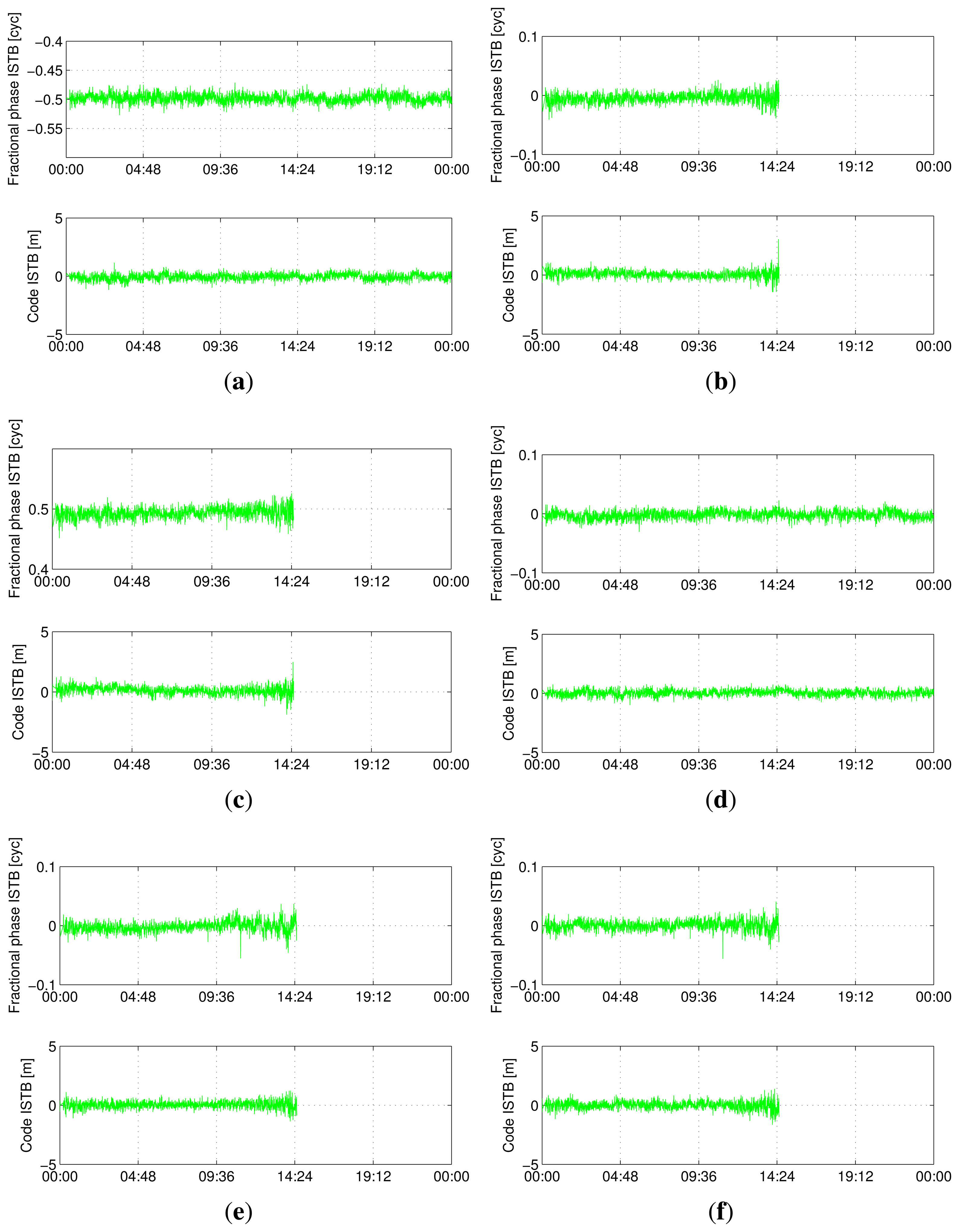
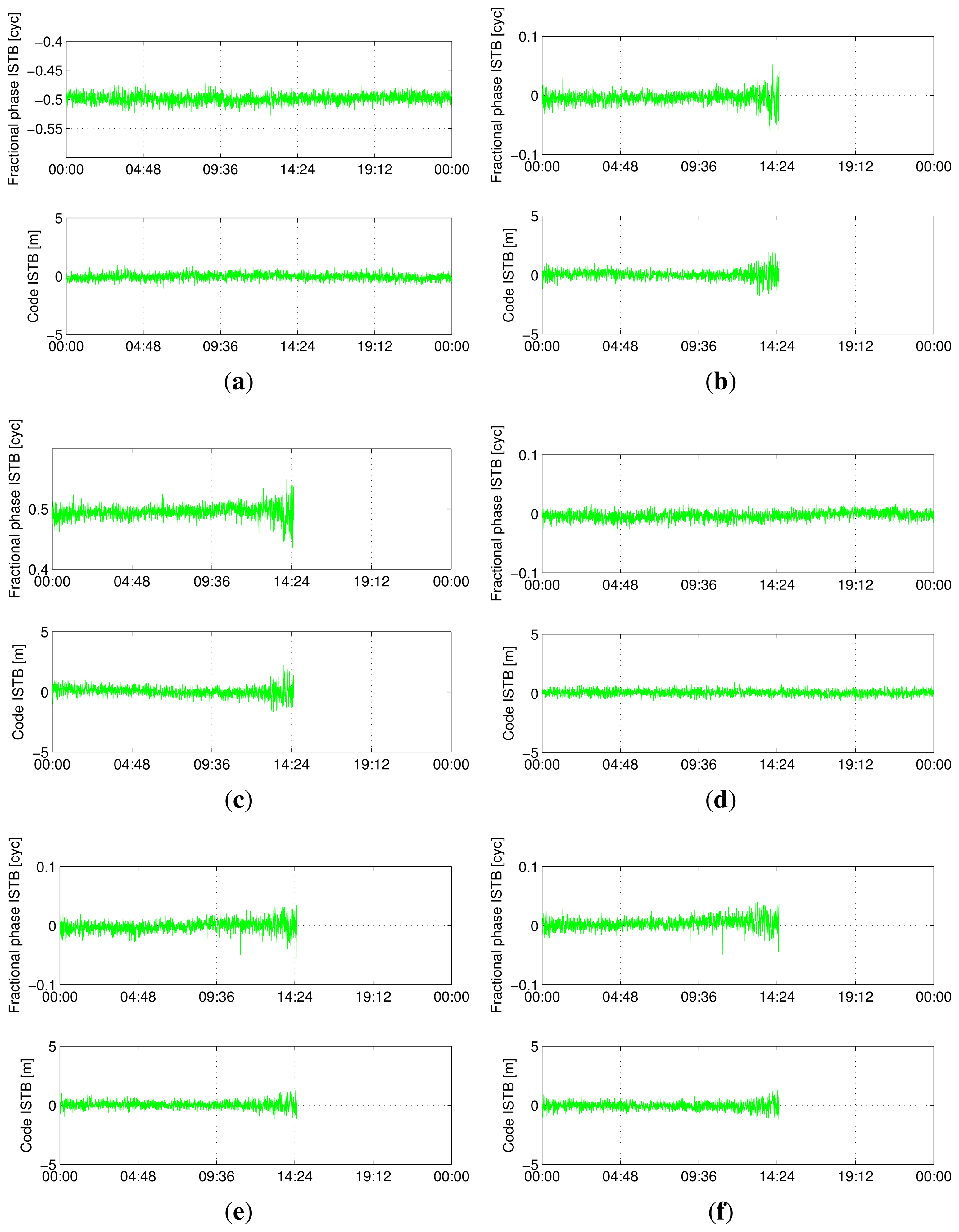
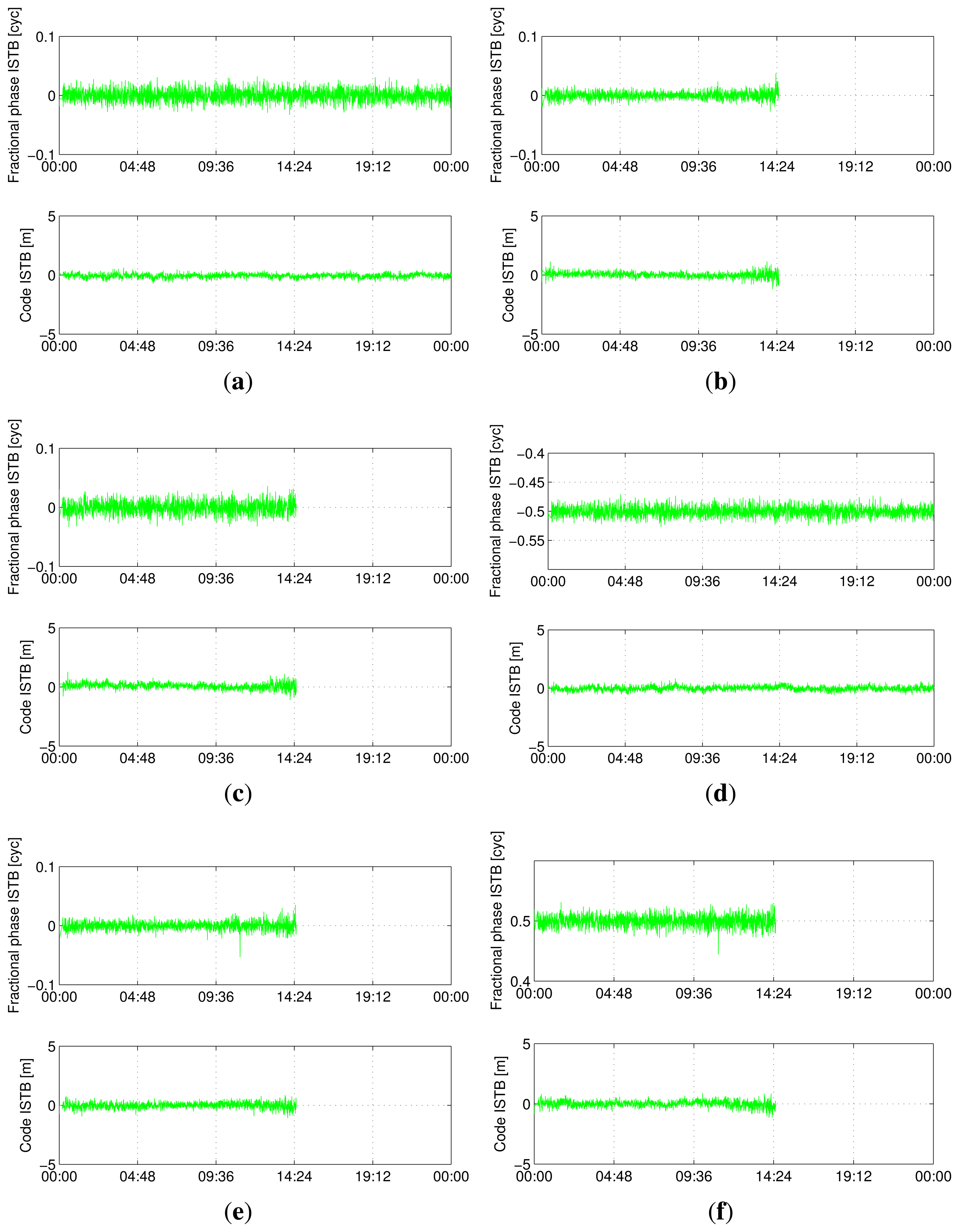
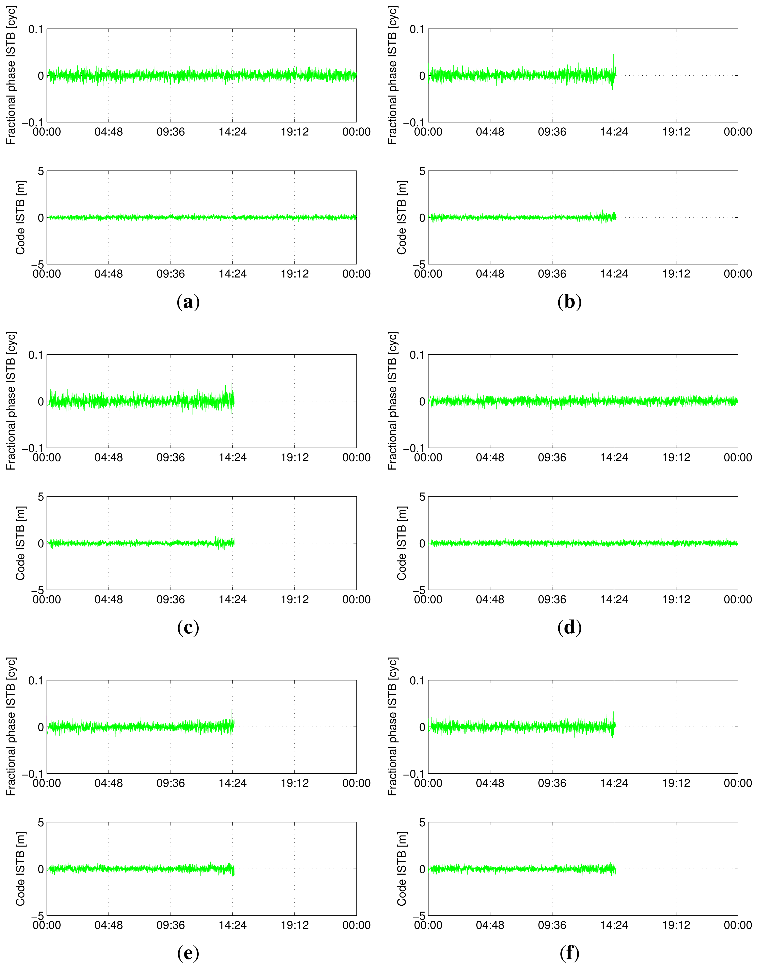
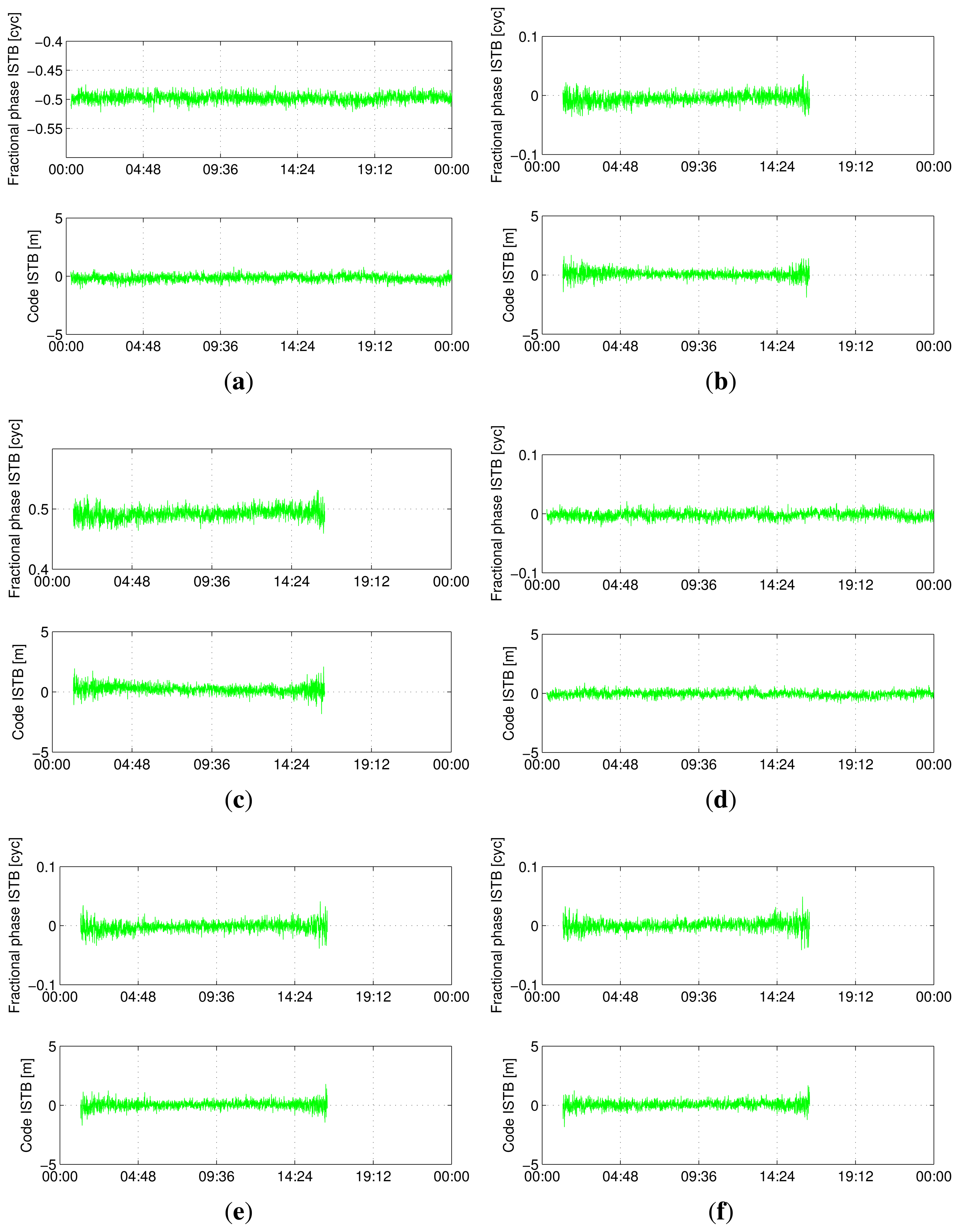
Figure 5, 6, 7 and 8 show the time series of ISTB estimates for zero-baselines formed by Curtin receivers (CUT0-CUT1, CUT0-CUT2, CUT0-CUT3 and CUTA-CUAA) on April 4, 2013. The first two columns are for ISTBs of GEO and MEO satellite types with an IGSO satellite as the reference, while the last column is for MEO ISTBs with respect to GEO satellites. Similar results for Curtin's open space experiment are given in Figure 9, matching with the results of the same receiver pair (Trimble-Javad) in Figure 7 and 8. The gaps in the MEO-related time series are due to the unavailability of visible MEO satellites during those periods.
It is observed that the estimated ISTBs (monitored for several days) are very stable and can be used to calibrate BeiDou observations. In the following, we compute the ISTB corrections using epoch-by-epoch estimates of several days. Let us consider the time series of the ith ITSB and associated standard deviations, where K is the number of epochs and hi:k is the estimated code or phase ISTB at time k. Assuming these estimates are uncorrelated over time, we formulate the following least-squares problem for the bias estimation:
Table 5 and 6 summarize the ISTB estimates and their standard deviations, clearly indicating the existence of non-zero ISTBs (highlighted using bold text) between dissimilar receiver types. It was observed that the estimated ISTBs are constant for given receiver-antenna connectivity and receiver operating environment. Nevertheless, it was found that the observed code ISTBs do not significantly affect ambiguity resolution and the consequent ambiguity resolved phase-only baseline estimation. However, the phase ISTBs severely affect ambiguity resolution, especially in the case of half-cycle phase ISTBs. As summarized in Table 7, GEO satellites have phase ISTBs of half-cycles with respect to IGSO/MEO satellites in the case of mixed receivers. Note that phase ISTBs for other receiver pairs can be deduced from estimates in Table 7. For example, with the sign convention in Table 4, the Septentrio-Javad pair has phase ISTBs of -0.5 cycle and 0.5 cycle for B1 and B2, respectively. Note that, for attitude determination with the ISTB-corrected model in the following section, we only correct phase observations with half cycles, as other (code) biases were found to be small enough to not affect the ambiguity resolution significantly.
4.3. Effect of ISTBs on Attitude Determination
Next, we analysed the impact of ISTBs on BeiDou single- and dual-frequency instantaneous attitude determination using the standard LAMBDA and C-LAMBDA methods comparing three processing approaches, namely, the classical DD model with ignoring ISTBs in Equation (19), the extended model in Equation (26) and the classical DD model with ISTB correction in Equation (28). Results for different receiver pairs (CUT0-CUTA, CUT0-CUAA, CUT1-CUTA and CUT1-CUAA), which consist of mixed receivers forming a short baseline of 8.418 m, as shown in Figure 1b, are discussed in the following. Note that these receiver pairs are not used in the computation of ISTBs in Section 4.2. We considered two performance measures for our analyses; the first one is the empirical instantaneous ambiguity success fraction (relative frequency), which is defined as:
Table 8, 9 and 10 report the instantaneous ambiguity success fraction for single-frequency B1, single-frequency B2 and dual frequency B1-B2 processing, respectively. The first row in each table corresponds to the baseline with the same receiver type for which ISTBs are zero and correction is not needed. The third row in Table 8 and the second row in Table 9 correspond to baselines with dissimilar receiver types, which have zero ISTBs for corresponding frequencies. The benefits of using C-LAMBDA, which makes use of known baseline length, are highlighted using bold text. Furthermore, catastrophic failures of ambiguity resolution by ignoring non-zero ISTBs are highlighted with emphasized text. Hence, it is wise to use the extended model (or the type-specific DD model) if one does not have the knowledge of ISTB between dissimilar receiver pairs. However, the best processing strategy is to use ISTB-corrected classical double differencing. With ISTB calibration, the C-LAMBDA method yields single-frequency instantaneous attitude determination.
Finally, Table 11 reports ambiguity fixed angular accuracy for single- and dual-frequency processing. Since the baselines (8.418 m) considered in these analyses are formed by receivers with similar noise characteristics, the ambiguity fixed angular standard deviations are the same for all cases, except the cases with catastrophic failure of ambiguity resolution. Hence, we report the average angular standard deviation of all other cases. Single-frequency processing with either B1 or B2 yields the same angular accuracy. The improved dual-frequency angular accuracy reflects the increased redundancy.
5. Summary and Conclusions
In this contribution, we investigated the existence of BeiDou inter-satellite-type biases (ISTBs) and their impact on standalone BeiDou attitude determination with mixed receiver types. We considered an extended GNSS double difference model incorporating all possible differential ISTBs among the three BeiDou satellite types (GEO, IGSO and MEO), together with three processing approaches, namely, one based on the classical double differenced model, ignoring the ISTBs, another based on the extended double differenced model, incorporating the ISTBs, and a third one based on the ISTB-corrected classical double differenced model. Our analyses using two real data sets with three different receiver types demonstrate the existence of non-zero ISTBs between different satellite types. The estimated ISTBs are stable and can be used to correct mixed receiver BeiDou attitude determination. It was observed that the estimated ISTBs are constant for a given receiver-antenna connectivity and receiver operating environment. Nevertheless, it was found that the observed code ISTBs do not significantly affect ambiguity resolution and the consequent ambiguity resolved phase-only baseline estimation. However, the mixed receiver half-cycle phase ISTBs severely affect ambiguity resolution. This finding is an important warning for mixed receiver type users, including precise point positioning users [54,55,57,58]. Moreover, it may also trigger GNSS receiver manufacturers to develop mutually consistent measurement extractions, as they are in the early stage of BeiDou-enabled receiver developments. Furthermore, it is suggested to use the extended model or, equivalently, the type-specific DD model, if one does not have the knowledge of ISTBs between dissimilar receiver pairs. However, the best processing strategy is to use the ISTB-corrected classical double differencing procedure. With ISTB correction, the C-LAMBDA method enables single-frequency, instantaneous attitude determination capability in the Asia-Pacific region with the current BeiDou constellation.
Acknowledgments
This work is supported by the Australian Space Research Program GARADA project on SAR For-mation Flying. The second author, P.J.G. Teunissen, is the recipient of an Australian Research Council Federation Fellowship (project number FF0883188). All this support is gratefully acknowledged.
Conflict of Interest
The authors declare no conflict of interest.
References
- CSNO. BeiDou Navigation Satellite System Signal in Space Interface Control Document: Open Service Signal B1I; Version 1.0; China Satellite Navigation Office: Beijing, China; December; 2012. [Google Scholar]
- Cao, C.; Jing, G.; Luo, M. COMPASS Satellite Navigation System Development. PNT Challenges and Opportunities Symposium, Stanford, CA, USA, 5–6 November 2008.
- Grelier, T.; Ghion, A.; Dantepal, J.; Ries, L.; de Latour, A.; Issler, J.L.; Avila-Rodriguez, J.; Wallner, S.; GW, H. COMPASS signal structure and first measurements. ION GNSS 2007, 2007, 3015–3024. [Google Scholar]
- Chen, H.; Huang, Y.; Chiang, K.; Yang, M.; Rau, R. The performance comparison between GPs and BeiDou-2/COMPASS: A perspective from Asia. J. Chin. Inst. Eng. 2009, 32, 679–689. [Google Scholar]
- Yang, Y.; Li, J.; Xu, J.; Tang, J.; Guo, H.; He, H. Contribution of the Compass satellite navigation system to global PNT users. Chin. Sci. Bull. 2011, 56, 2813–2819. [Google Scholar]
- Zhang, S.; Guo, J.; Li, B.; Rizos, C. An Analysis of Satellite Visibility and Relative Positioning Precision of COMPASS. Proceedings of Symposium for Chinese Professionals in GPS, Shanghai, China, 18–20 August 2011; pp. 41–46.
- Verhagen, S.; Teunissen, P.J. Ambiguity resolution performance with GPS and BeiDou for LEO formation flying. Adv. Space Res. 2013. [Google Scholar] [CrossRef]
- Montenbruck, O.; Hauschild, A.; Steigenberger, P.; Hugentobler, U.; Teunissen, P.J.G.; Nakamura, S. Initial assessment of the COMPASS/BeiDou-2 regional navigation satellite system. GPS Solut. 2013, 17, 211–222. [Google Scholar]
- Montenbruck, O.; Hauschild, A.; Steigenberger, P.; Hugentobler, U.; Riley, S. A COMPASS for Asia: First Experience with the BeiDou-2 Regional Navigation System. IGS Workshop, Olsztyn, Poland, 23–27 July 2012.
- Shi, C.; Zhao, Q.; Li, M.; Tang, W.; Hu, Z.; Lou, Y.; Zhang, H.; Niu, X.; Liu, J. Precise orbit determination of BeiDou Satellites with precise positioning. Sci. China Earth Sci. 2012, 55, 1079–1086. [Google Scholar]
- Steigenberger, P.; Hauschild, A.; Montenbruck, O.; Hugentobler, U. Performance Analysis of COMPASS Orbit and Clock Determination and COMPASS-only PPP. IGS Workshop, Olsztyn, Poland, 23–27 July 2012.
- Odolinski, R.; Teunissen, P.J.G.; Odijk, D. An Analysis of Combined COMPASS/BeiDou-2 and GPS Single- and Multiple-Frequency RTK Positioning. Proceedings of the Institute of Navigation Pacific PNT 2013, Honolulu, HI, USA, 22–25 April 2013; pp. 69–90.
- Cai, C.; Gao, Y.; Pan, L.; Dai, W. An analysis on combined GPS/COMPASS data quality and its effect on single point positioning accuracy under different observing conditions. Adv. Space Res. 2013. [Google Scholar] [CrossRef]
- Li, W.; Teunissen, P.J.G.; Zhang, B.; Verhagen, S. Precise Point Positioning Using GPS and Compass Observations. Proceedings of the 4th China Satellite Navigation Conference (CSNC), Wuhan, China, 15–17 May 2013.
- Zhao, Q.; Guo, J.; Li, M.; Qu, L.; Hu, Z.; Shi, C.; Liu, J. Initial results of precise orbit and clock determination for COMPASS navigation satellite system. J. Geod. 2013, 87, 475–486. [Google Scholar]
- Nadarajah, N.; Teunissen, P.J.G.; Buist, P.; Steigenberger, P. First Results of Instantaneous GPS/Galileo/COMPASS Attitude Determination. Proceedings of the 6th ESA Workshop on Satellite Navigation User Equipment Technologies, Noordwijk, The Netherlands, 5–7 December 2012; p. 8.
- Nadarajah, N.; Teunissen, P.J.G. Instantaneous GPS/BeiDou/Galileo Attitude Determination: A Single-Frequencyr Robustness Analysis under Constrained Environments. Proceedings of The Institute of Navigation Pacific PNT, Honolulu, HI, USA, 22–25 April, 2013; pp. 1088–1103.
- Nadarajah, N.; Teunissen, P.J.G.; Raziq, N. Instantaneous COMPASS-GPS attitude determination: A robustness analysis. Adv. Space Res 2013. submitted. [Google Scholar]
- Shi, C.; Zhao, Q.; Hu, Z.; Liu, J. Precise relative positioning using real tracking data from COMPASS GEO and IGSO satellites. GPS Solut. 2013, 17, 103–119. [Google Scholar]
- Steigenberger, P.; Hauschild, A.; Montenbruck, O.; Rodriguez-Solano, C.; Hugentobler, U. Orbit and clock determination of QZS-1 based on the CONGO network. ION-ITM-2012. 2012. [Google Scholar]
- Steigenberger, P.; Hugentobler, U.; Hauschild, A.; Montenbruck, O. Orbit and clock analysis of Compass GEO and IGSO satellites. J. Geod. 2013, 87, 515–525. [Google Scholar]
- Cohen, C. Attitude Determination Using GPS. Ph.D. Thesis, Stanford University, Stanford, CA, USA, 1992. [Google Scholar]
- Lu, G. Development of A GPS Multi-Antenna System for Attitude Determination. Ph.D. Thesis, University of Calgary, Calgary, Alberta, Canada, 1995. [Google Scholar]
- Crassidis, J.L.; Markley, F.L. New algorithm for attitude determination using Global Positioning System signals. J. Guidance Control Dyn. 1997, 20, 891–896. [Google Scholar]
- Li, Y.; Zhang, K.; Roberts, C.; Murata, M. On-the-fly GPS-based attitude determination using single- and double-differenced carrier phase measurements. GPS Solut. 2004, 8, 93–102. [Google Scholar]
- Lin, D.; Voon, L.; Nagarajan, N. Real-time Attitude Determination for Microsatellite by LAMBDA Method Combined with Kalman Filtering. Proceedings of the 22nd AIAA International Communications Satellite Systems Conference and Exhibit, Monterey, California, USA, 9–12 May 2004.
- Madsen, J.; Lightsey, E.G. Robust spacecraft attitude determination using global positioning system receivers. J. Spacecr. Rocket. 2004, 41, 635–643. [Google Scholar]
- Psiaki, M.L. Batch algorithm for global-positioning-system attitude determination and integer ambiguity resolution. J. Guidance Control Dyn. 2006, 29, 1070–1079. [Google Scholar]
- Teunissen, P.J.G. The least-squares ambiguity decorrelation adjustment: A method for fast GPS integer ambiguity estimation. J. Geod. 1995, 70, 65–82. [Google Scholar]
- Boon, F.; Ambrosius, B. Results of Real-time Applications of the LAMBDA Method in GPS Based Aircraft Landings. Proceedings of the International Symposium on Kinematic Systems in Geodesy, Geomatics and Navigation, Banff, AB, Canada, 3–6 June 1997; pp. 339–345.
- Cox, D.B.; Brading, J.D.W. Integration of LAMBDA Ambiguity Resolution with Kalman Filter for Relative Navigation of Spacecraft. Proceedings of the 55th Annual Meeting of The Institute of Navigation, Cambridge, MA, USA, 27–30 June, 1999; pp. 739–745.
- Ji, S.; Chen, W.; Zhao, C.; Ding, X.; Chen, Y. Single epoch ambiguity resolution for Galileo with the CAR and LAMBDA methods. GPS Solut. 2007, 11, 259–268. [Google Scholar]
- Huang, S.; Wang, J.; Wang, X.; Chen, J. The application of the LAMBDA method in the estimation of the GPS slant wet vapour. Acta Astron. Sinica 2009, 50, 60–68. [Google Scholar]
- Kroes, R.; Montenbruck, O.; Bertiger, W.; Visser, P. Precise GRACE baseline determination using GPS. GPS Solutions 2005, 9, 21–31. [Google Scholar]
- Jin, S.; Luo, O.; Ren, C. Effects of physical correlations on long-distance GPS positioning and zenith tropospheric delay estimates. Adv. Space Res. 2010, 46, 190–195. [Google Scholar]
- Jin, S.; Wang, J.; Park, P.H. An improvement of GPS height estimations-Stochastic modeling. Earth Planets Space 2005, 57, 253–259. [Google Scholar]
- Park, S.Y. Thermally induced attitude disturbance control for spacecraft with a flexible boom. J. Spacecr. Rocket. 2002, 39, 325–328. [Google Scholar]
- Teunissen, P.J.G. An optimality property of the integer least-squares estimator. J. Geod. 1999, 73, 587–593. [Google Scholar]
- Teunissen, P.J.G.; De Jonge, P.; Tiberius, C. Performance of the LAMBDA method for fast GPS ambiguity resolution. Navigation 1997, 44, 373–383. [Google Scholar]
- Verhagen, S.; Teunissen, P.J.G. New global navigation satellite system ambiguity resolution method compared to existing approaches. J. Guidance Control Dyn. 2006, 29, 981–991. [Google Scholar]
- Park, C.; Teunissen, P.J.G. A New Carrier Phase Ambiguity Estimation for GNSS Attitude Determination Systems. Proceedings of International Symposium on GPS/GNSS, Tokyo, Japan, 15–18 November 2003; pp. 283–290.
- Teunissen, P.J.G. The LAMBDA method for the GNSS compass. Artif. Satell. 2006, 41, 89–103. [Google Scholar]
- Buist, P.J. The Baseline Constrained LAMBDA Method for Single Epoch, Single Frequency Attitude Determination Applications. Proceedings of the 20th International Technical Meeting of the Satellite Division of the Institute of Navigation (ION GNSS 2007), Fort Worth, TX, USA, 25–28 September 2007; pp. 2962–2973.
- Park, C.; Teunissen, P.J.G. Integer least squares with quadratic equality constraints and its application to GNSS attitude determination systems. Int. J. Control Autom. Syst. 2009, 7, 566–576. [Google Scholar]
- Giorgi, G.; Teunissen, P.J.G.; Buist, P.J. A Search and Shrink Approach for the Baseline Constrained LAMBDA Method: Experimental Results. Proceedings of International Symposium on GPS/GNSS, Tokyo, Japan, 11–14 November 2008; pp. 797–806.
- Giorgi, G.; Buist, P. Single-epoch, Single-frequency, Standalone Full Attitude Determination: Experimental Results. Proceedings of the 4th ESA Workshop on Satellite Navigation User Equipment Technologies, NAVITEC, Noordwijk, The Netherlands, 10–12 December; p. 8.
- Teunissen, P.J.G. Integer least-squares theory for the GNSS compass. J. Geod. 2010, 84, 433–447. [Google Scholar]
- Giorgi, G.; Teunissen, P.J.G.; Verhagen, S.; Buist, P.J. Testing a new multivariate GNSS carrier phase attitude determination method for remote sensing platforms. Adv. Space Res. 2010, 46, 118–129. [Google Scholar]
- Teunissen, P.J.G.; Giorgi, G.; Buist, P.J. Testing of a new single-frequency GNSS carrier phase attitude determination method: Land, ship and aircraft experiments. GPS Solut. 2011, 15, 15–28. [Google Scholar]
- Teunissen, P.J.G.; Kleusberg, A. GPS for Geodesy, 2nd ed.; Springer: Berlin/Heidelberg, Germany, 1998. [Google Scholar]
- Harville, D.A. Matrix Algebra From A Statistician's Perspective; Springer: New York, NY, USA, 1997. [Google Scholar]
- Magnus, J.R.; Neudecker, H. Matrix Differential Calculus with Applications in Statistics and Econometrics; Wiley: New York, NY, USA, 1995. [Google Scholar]
- Teunissen, P.J.G. Zero Order Design : Generalized Inverses, Adjustment, the Datum Problem and S-transformations. In Optimization and Design of Geodetic Networks; Grafarend, E., Sans, F., Eds.; Springer: Berlin/Heidelberg, Germany, 1985; pp. 11–55. [Google Scholar]
- Teunissen, P.J.G.; Odijk, D.; Zhang, B. PPP-RTK: Results of CORS network-based PPP with integer ambiguity resolution. J. Aeronaut. Astronaut. Aviat. Series A 2010, 42, 223–230. [Google Scholar]
- Odijk, D.; Teunissen, P.J.G.; Zhang, B. Single-frequency integer ambiguity resolution enabled precise point positioning. J. Surv. Eng. 2012, 138, 193–202. [Google Scholar]
- Euler, H.J.; Goad, C. On optimal filtering of GPS dual frequency observations without using orbit information. J. Geod. 1991, 65, 130–143. [Google Scholar]
- Geng, J.; Meng, X.; Dodson, A.; Teferle, F. Integer ambiguity resolution in precise point positioning: Method comparison. J. Geod. 2010, 84, 569–581. [Google Scholar]
- Zhang, B.; Teunissen, P.J.G.; Odijk, D. A novel un-differenced PPP-RTK concept. J. Navig. 2011, 64, S180–S191. [Google Scholar]


| Model | Redundancy |
|---|---|
| Classical DD with ignoring ISTBs Equation (19) | f(m − 1) −3 |
| Extended model (26) | f(m − η) − 3 |
| Type-specific DD model (27) | f(m − η) − 3 |
| Classical DD with ISTB correction Equation (28) | f(m − 1) − 3 |
| Experiments | Duration |
|---|---|
| Curtin 1 | April 19–21 |
| Curtin 2 | April 29–May 01 |
| Kalamunda 1 | May 19–21 |
| Kalamunda 2 | May 29–31 |
| Frequency | Code | Phase | ||||
|---|---|---|---|---|---|---|
| σpo [cm] | apo | ϵpo [deg] | σΦo [mm] | aΦo | ϵΦo [deg] | |
| B1 and B2 | 20 | 5 | 15 | 2 | 5 | 15 |
| Satellite type pairs | Rounding method/Sign |
|---|---|
| GEO-IGSO | floor/+ |
| GEO-MEO | floor/+ |
| IGSO-GEO | ceiling/− |
| IGSO-MEO | ceiling/− |
| MEO-GEO | ceiling/+ |
| MEO-IGSO | floor/− |
| Receiver Pair | Frequency | IGSO-GEO | IGSO-MEO | GEO-MEO | |||
|---|---|---|---|---|---|---|---|
| Phase ISTB/std (cyc) | Code ISTB/std (m) | Phase ISTB/std (cyc ) | Code ISTB/std (m) | Phase ISTB/std (cyc) | Code ISTB/std (m) | ||
| CUT0-CUT1 | B1 | 0.00/ 0.000 | −0.07/ 0.002 | 0.00/ 0.000 | 0.03/ 0.003 | 0.00/ 0.000 | 0.10/ 0.003 |
| (Trimble-Septentrio) | B2 | −0.50/ 0.000 | −0.01/ 0.002 | 0.00/ 0.000 | 0.01/ 0.003 | 0.50/ 0.000 | 0.02/ 0.003 |
| CUT0-CUT2 | B1 | 0.00/ 0.000 | 0.00/ 0.002 | 0.00/ 0.000 | 0.00/ 0.003 | 0.00/ 0.000 | 0.00/ 0.003 |
| (Trimble-Trimble) | B2 | 0.00/ 0.000 | 0.00/ 0.002 | 0.00/ 0.000 | 0.00/ 0.003 | 0.00/ 0.000 | 0.00/ 0.003 |
| CUT0-CUT3 | B1 | −0.50/ 0.000 | −0.06/ 0.002 | 0.00/ 0.000 | 0.04/ 0.003 | 0.49/ 0.000 | 0.10/ 0.003 |
| (Trimble-Javad) | B2 | −0.00/ 0.000 | 0.03/ 0.002 | 0.00/ 0.000 | 0.05/ 0.003 | 0.00/ 0.000 | 0.01/ 0.004 |
| CUTA-CUAA | B1 | −0.50/ 0.000 | −0.06/ 0.002 | 0.00/ 0.000 | 0.01/ 0.003 | 0.50/ 0.000 | 0.07/ 0.003 |
| (Trimble-Javad) | B2 | 0.00/ 0.000 | 0.04/ 0.002 | 0.00/ 0.000 | 0.03/ 0.003 | 0.00/ 0.000 | −0.02/ 0.003 |
| Experiment | Frequency | IGSO-GEO | IGSO-MEO | GEO-MEO | |||
|---|---|---|---|---|---|---|---|
| Phase ISTB/std(cyc) | Code ISTB/std (m) | Phase ISTB/std(cyc) | Code ISTB/std (m) | Phase ISTB/std(cyc) | Code ISTB/std (m) | ||
| Curtin 1 | B1 | −0.50/0.000 | −0.17/0.003 | 0.00/0.000 | 0.06/0.005 | 0.49/0.000 | 0.23/0.005 |
| B2 | 0.00/0.000 | −0.06/0.003 | 0.00/0.000 | 0.04/0.005 | 0.00/0.000 | 0.10/0.005 | |
| Curtin 2 | B1 | −0.50/0.000 | −0.16/0.003 | 0.00/0.000 | 0.05/0.006 | 0.49/0.000 | 0.20/0.006 |
| B2 | 0.00/0.000 | −0.06/0.003 | 0.00/0.000 | 0.03/0.006 | 0.00/0.000 | 0.08/0.006 | |
| Kalamunda 1 | B1 | −0.50/0.000 | −0.12/0.003 | 0.00/0.000 | 0.04/0.005 | 0.49/0.000 | 0.16/0.005 |
| B2 | 0.00/0.000 | −0.03/0.003 | 0.00/0.000 | 0.03/0.005 | 0.00/0.000 | 0.06/0.005 | |
| Kalamunda 2 | B1 | −0.50/0.000 | −0.11/0.003 | 0.00/0.000 | 0.04/0.005 | 0.49/0.000 | 0.16/0.005 |
| B2 | 0.00/0.000 | −0.02/0.003 | 0.00/0.000 | 0.04/0.005 | 0.00/0.000 | 0.07/0.005 | |
| Frequency | Trimble | Septentrio | Javad |
|---|---|---|---|
| B1 | 0 | 0 | −0.5 |
| B2 | 0 | −0.5 | 0 |
| Baseline | Classical DD model Equation (19) | Extended model Equation (26) | Classical DD model with ISTB correction Equation (28) | |||
|---|---|---|---|---|---|---|
| LAMBDA | C-LAMBDA | LAMBDA | C-LAMBDA | LAMBDA | C-LAMBDA | |
| CUT0-CUTA (Trimble-Trimble) | 0.98 | 1.00 | 0.77 | 0.99 | 0.98 | 1.00 |
| CUT0-CUAA (Trimble-Javad) | 0.00 | 0.00 | 0.75 | 0.99 | 0.97 | 1.00 |
| CUT1-CUTA (Septentrio-Trimble) | 0.99 | 1.00 | 0.87 | 1.00 | 0.99 | 1.00 |
| CUT1-CUAA (Septentrio-Javad) | 0.00 | 0.00 | 0.86 | 1.00 | 0.99 | 1.00 |
| Baseline | Classical DD model Equation (19) | Extended model Equation (26) | Classical DD model with ISTB correction Equation (28) | |||
|---|---|---|---|---|---|---|
| LAMBDA | C-LAMBDA | LAMBDA | C-LAMBDA | LAMBDA | C-LAMBDA | |
| CUT0-CUTA (Trimble-Trimble) | 0.98 | 1.00 | 0.86 | 1.00 | 0.98 | 1.00 |
| CUT0-CUAA (Trimble-Javad) | 0.99 | 1.00 | 0.88 | 1.00 | 0.99 | 1.00 |
| CUT1-CUTA (Septentrio-Trimble) | 0.00 | 0.00 | 0.94 | 1.00 | 0.99 | 1.00 |
| CUT1-CUAA (Septentrio-Javad) | 0.00 | 0.00 | 0.96 | 1.00 | 1.00 | 1.00 |
| Baseline | Classical DD model Equation (19) | Extended model Equation (26) | Classical DD model with ISTB correction Equation (28) | |||
|---|---|---|---|---|---|---|
| LAMBDA | C-LAMBDA | LAMBDA | C-LAMBDA | LAMBDA | C-LAMBDA | |
| CUT0-CUTA (Trimble-Trimble) | 1.00 | 1.00 | 1.00 | 1.00 | 1.00 | 1.00 |
| CUT0-CUAA (Trimble-Javad) | 0.00 | 0.00 | 1.00 | 1.00 | 1.00 | 1.00 |
| CUT1-CUTA (Septentrio-Trimble) | 0.00 | 0.00 | 1.00 | 1.00 | 1.00 | 1.00 |
| CUT1-CUAA (Septentrio-Javad) | 0.00 | 0.00 | 1.00 | 1.00 | 1.00 | 1.00 |
| Single-Frequency (B1) | Single-Frequency (B2) | Dual-Frequency (B1–B2) | |
|---|---|---|---|
| Heading | 0.02 (0.02) | 0.02 (0.02) | 0.01 (0.01) |
| Elevation | 0.04 (0.04) | 0.04 (0.04) | 0.03 (0.03) |
© 2013 by the authors; licensee MDPI, Basel, Switzerland. This article is an open access article distributed under the terms and conditions of the Creative Commons Attribution license (http://creativecommons.org/licenses/by/3.0/).
Share and Cite
Nadarajah, N.; Teunissen, P.J.G.; Raziq, N. BeiDou Inter-Satellite-Type Bias Evaluation and Calibration for Mixed Receiver Attitude Determination. Sensors 2013, 13, 9435-9463. https://doi.org/10.3390/s130709435
Nadarajah N, Teunissen PJG, Raziq N. BeiDou Inter-Satellite-Type Bias Evaluation and Calibration for Mixed Receiver Attitude Determination. Sensors. 2013; 13(7):9435-9463. https://doi.org/10.3390/s130709435
Chicago/Turabian StyleNadarajah, Nandakumaran, Peter J. G. Teunissen, and Noor Raziq. 2013. "BeiDou Inter-Satellite-Type Bias Evaluation and Calibration for Mixed Receiver Attitude Determination" Sensors 13, no. 7: 9435-9463. https://doi.org/10.3390/s130709435
APA StyleNadarajah, N., Teunissen, P. J. G., & Raziq, N. (2013). BeiDou Inter-Satellite-Type Bias Evaluation and Calibration for Mixed Receiver Attitude Determination. Sensors, 13(7), 9435-9463. https://doi.org/10.3390/s130709435