A Linear, Millimetre Displacement-to-Frequency Transducer

Abstract
: The paper presents a novel linear, high-fidelity millimetre displacement-to-frequency transducer, based on the resistive conversion of displacement into a proportional voltage, and then frequency. The derivation of the nonlinearity, fidelity and sensitivity of the transducer is presented. Experimental results confirm that a displacement of 0–100 mm is converted into a frequency range of 0–100 kHz, with a normalised fidelity factor of 99.91%, and a worst-case nonlinearity of less than 0.08%. Tests using laboratory standards show that a displacement of 10 mm is transduced with an accuracy of ±0.6%, and a standard deviation of 530 Hz. Estimates included in the paper show that the transducer could cost less than 1% of existing systems for millimeter displacement measurement.1. Introduction
Several ultrasound, optical or laser-based devices exist for the measurement of displacements larger than one metre [1–4]. The cost of the modifications required for the use of these systems for measuring displacements in the range of a few micrometres to millimetres (submetre) is only justifiable in a few circumstances. For affordable submetre displacement measurements, capacitive and inductive position sensors are often used. However, the frequency dependence of capacitive and inductive sensors limits their domains of application [5–7]. In fact, a comparative discourse relating the range of displacement measurable versus the sensor recommended, could be found in [8].
In process and industrial instrumentation systems, several variables are detected using elastic sensors as primary sensing elements. Elastic sensors often generate displacements in the range of several micrometres to millimeters, which have to be conditioned further. Table 1, derived from information available in Chapter 8 of [9], shows example applications of elastic sensors resulting in an intermediate displacement variable. Moreover, physiological changes in biological tissues resulting from dehydration, accumulation of fluid due to disease, etc., can be studied using submetre displacement measurements [10]. Millimeter displacement is also encountered in the analysis of the integrity of civil structures [11,12], where such measurement systems as the GPS-RTS are currently used. A key challenge in the current systems for millimeter-displacement measurement is the high cost of acquisition of such measurement systems. Hence, there is significant motivation for the exploration of cheaper systems for use in small displacement measurement. Moreover, the transducers most suitable for the conditioning of such small displacement signals must have high sensitivity, high fidelity and minimum nonlinearity for acceptable accuracy of transduction. This paper presents the design, analysis and experimental validation of a submetre displacement-to-frequency transducer. The system is based on the sensitivity of some resistive elements to displacement. Resistive sensors are relatively cheap; and their zero-order dynamics make them suitable for both static and dynamic measurements. Unlike time-of-flight devices or phase-based measurement systems, resistive millimeter displacement transducers need be coupled physically to the displacement being measured.
In the rest of the paper, the circuit design, analysis of the basic displacement-to-voltage converter, and the implementation of the primary conditioning amplifier circuit are presented in Section 2. The voltage-to-frequency conversion design is presented in Section 3 of the paper. Circuit realisation, experimental results, and discussions of these results form Section 4 of the paper. Section 5 presents conclusions and the limitation of the transducer circuit. A list of references concludes the paper.
2. The Basic Displacement Sensor, and the Design and Analysis of the Primary Conditioning Circuit
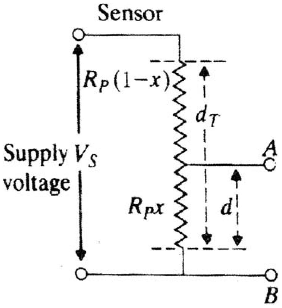
The basic displacement-to-voltage sensor is shown in Figure 1. The sensor consists of a three-terminal potentiometer of total resistance RP, supplied by a DC voltage Vs. The resistance between terminals A and B of the potentiometer is directly related to the displacement d(t) (alternatively, the normalised displacement x), where and d(t) = xdT. Then:
Note that, the maximum value of ETH is Vs, when x = 1. The Thevenin's resistance of the equivalent sensor circuit, RTH, is evaluated to yield [9]:
The sensitivity of ETH to the normalised displacement x is given by:
To avoid excessive power dissipation in the resistance of the potentiometer, Vs is usually kept small.
Consequently, the sensitivity of this basic sensor is small. Additional conditioning is required to improve the sensitivity of the sensor. Now, the normalised sensitivity is given by:
2.1. Primary Conditioning of Sensor Output
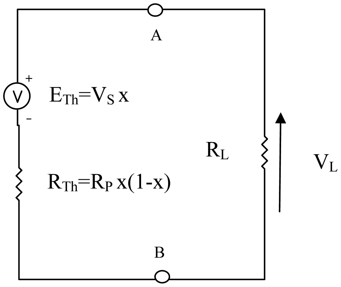
The equivalent circuit resulting from the connection of a primary amplifier of input resistance RL, across terminals AB of the sensor circuit is shown in Figure 2. Loading effects tend to degrade the performance of amplifiers. The loading effect of the conditioning circuit modifies the Thevenin's voltage to:
The normalised value of this voltage is also derived to be:
In the next sub-section of the paper, Equations (5) and (6) are used to analyse the quality of the displacement-to-voltage conversion amplifier, and to show any additional condition(s) that could be imposed on the conditioning circuit to further improve the performance of the transducer.
2.2. Quality Analysis of the Primary Conditioning Circuit
In this subsection, the analysis of the quality of the primary signal amplification, based on Equation (5), is presented.
2.2.1. Fidelity of Primary Amplifier
Fidelity is a measure of how faithfully a circuit has processed a given signal to minimize distortions. The concept of fidelity is usually used in the analysis of high frequency amplifiers. In the current paper, the concept of fidelity is used to quantify the loading effect of the primary conditioning amplifier on the signal produced by the sensor. Now, the voltage drop due to the loading effect of RL is obtained to be:
The normalised fidelity factor is then given as:
For perfect fidelity, K = 0. Practically, this requires that:
2.2.2. Sensitivity Analysis
The sensitivity of the conditioned output is derived to yield:
The normalised sensitivity is found to be:
It is required to select the value of K in such a manner, as to minimize variations within the range of measurements.
2.2.3. Nonlinearity Effects
From Equation (5)VL is nonlinear in x. The nonlinearity N(x) can be quantified by using:
Nonlinearity is not desirable, and is eliminated as in Equation (10). In fact, it is evident from Equations (9), (10) and (15) that K → 0 improves linearity and fidelity. This contradicts the requirement for enhanced sensitivity as in Equation (12), for which K → ∞.The approach in this paper is to select K → 0 for fidelity and linearity enhancement; and to effect sensitivity improvement using voltage to frequency conversion.
2.2.4. Practical Realisation of the Signal Conditioning Amplifier
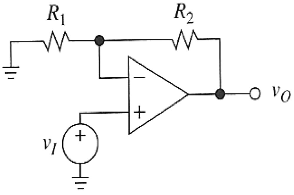
The practical implementation of the primary conditioning amplifier uses the summing amplifier shown in Figure 3 [13,14], with the amplified voltage given by:
An amplifier gain of 10 was used for the current work. This yields the normalised sensitivity parameter given in Equation (17).
Table 2 summarises the parameters of the sensor and the amplifying circuit.
Combining the parameter values in Table 2 with Equations (5) and (10) yields:
Therefore, within an accuracy of ±0.6%:
In Section 3, we present a technique to further improve the sensitivity of the transducer, using voltage-to-frequency conversion.
3. Sensitivity Enhancement
As observed above, a small value of K (0.0056) was required to both minimize nonlinearity effects, and to enhance fidelity of the primary conditioning circuit. This value of K however, lowers the sensitivity of the transduction process. Since submetre displacements can be very small, a very high sensitivity transducer is required (as shown in Table 2, ideal sensitivity required is ∞). In the sequel, we present a voltage-to-frequency converter circuit that is used to further enhance the sensitivity of the developed transducer.
3.1. Voltage-to-Frequency (VFC) Conversion
Apart from sensitivity enhancement, the conversion of v0 into a frequency signal has several other advantages, including: high noise immunity, high output power, wide dynamic range, and ease of interfacing with digital data acquisition systems. Table 3 shows key values of v0 and their corresponding frequency representations.
The linear relationship between v0 and frequency in Table 3 is expressed mathematically as:
Applying Equation (20) in Equation (22) we obtain:
It is evident from Equation (23) that:
The AD 650 voltage-to-frequency converter (VFC) was used for the implementation of the displacement-to-frequency conversion circuit satisfying Equation (23). The pin layout of the AD 650 VFC is obtained from the manufacturer's manual for the device [15]. The selection of components for the VFC circuit is presented in the sequel.
3.2. Component's Selection for the AD 650 VFC
For the AD 650, only four component values must be selected by the user [15]. Using the manufacturer's notation, these are the input resistance RIN, the timing capacitor COS, the logic resistor R2 and the integration capacitor CINT. The first two are determined by the input voltage range and full-scale frequency. Additional relationship between RIN and COS is provided through graphs obtainable in [15]. Sample design for a maximum frequency of 100 KHZ in the data sheet of the AD 650 VFC used RIN = 40 kΩ and this has been adopted for the realization in this study. Table 4 summarizes the components used for the design of the VFC circuit, with CINT calculated using the equation:
The frequency conversion improves the sensitivity of the transducer from the value given by Equation (17) to:
4. Simulations, Experimental Validation, Results Presentation and Discussions
The indices assessing the quality of the transducer were evaluated by simulation. The rest of the results were obtained through experimental measurements.
4.1. Simulations
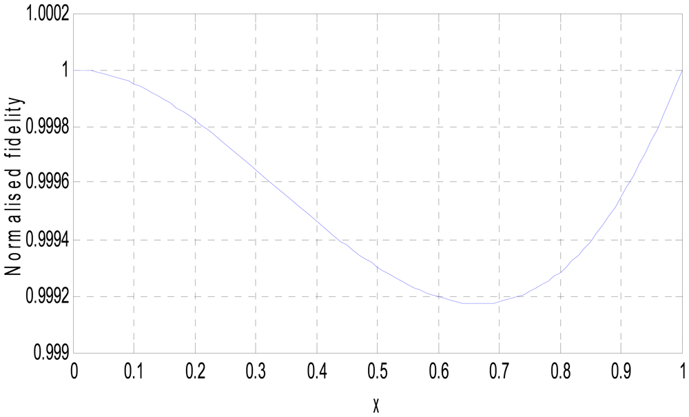
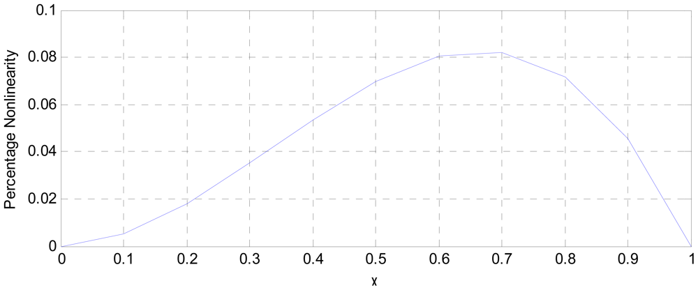
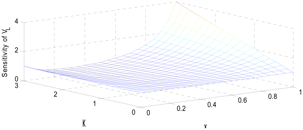
MATLAB simulation of the transducer fidelity, sensitivity and nonlinearity, based on Equations (9), (12) and (15) is presented in Figures 4–6.
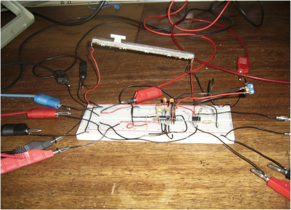
4.2. Experimental Validation
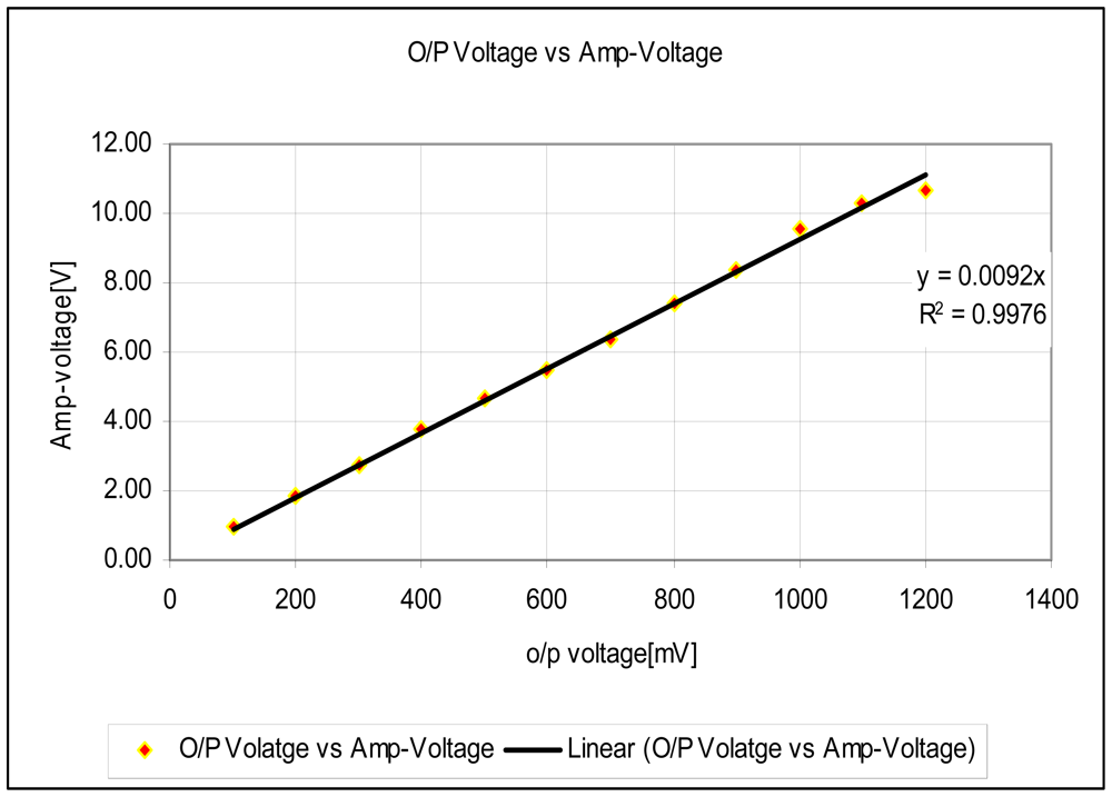
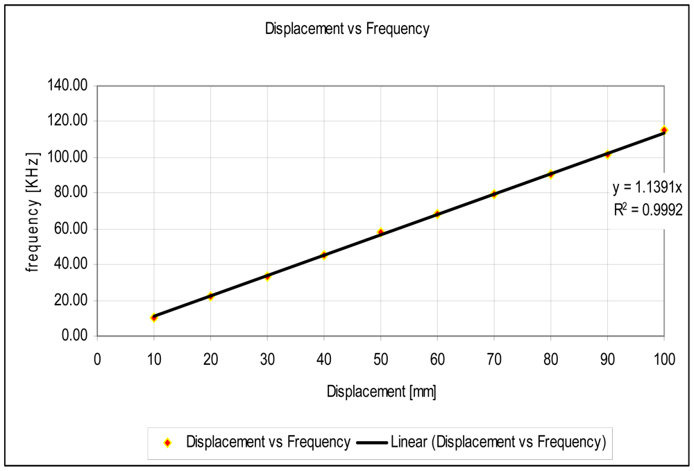
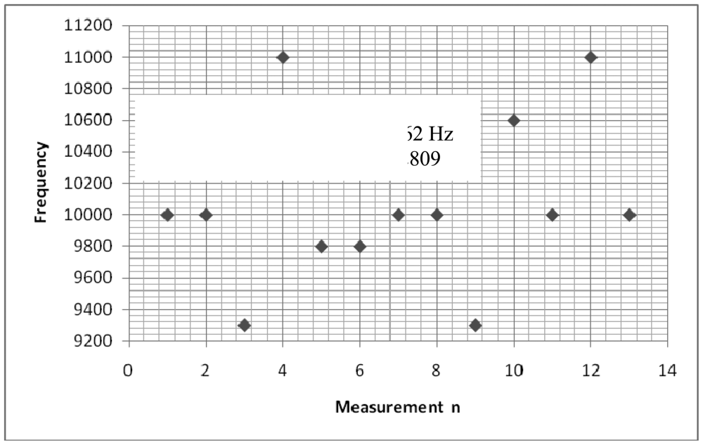
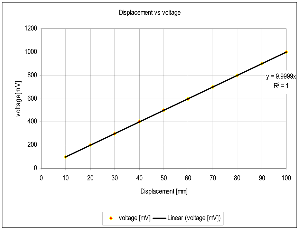
The experimental setup is shown in Figure 7. For the experiments, a slide wire potentiometer was used as the submeter displacement sensor. It had a maximum displacement dT = 100 mm = 10−1 m, and a total resistance of 11.2 kΩ (instead of the design maximum resistance of 10 kΩ). The potentiometer was supplied by a 1volt DC supply. The Thevenin voltage of the sensor, as a function of displacement, is shown in Figure 8. A plot of the amplified sensor voltage as function of detected displacement is shown in Figure 9. The overall displacement-to-frequency transduction is shown in Figure 10. For the analysis of the accuracy and precision of transducing displacement inputs into frequency, repeated measurements of 10 mm displacement were undertaken. The results are shown in Figures 11 and 12.
4.3. Result Discussions
The simulated fidelity results presented in Figure 4 shows that, the conditioning of the sensor signal by the primary amplifier was undertaken with at least 99.91% fidelity. Figure 5 shows that the introduction of the conditioning circuit slightly reduced the normalized input sensitivity to a value less than unity (0.988). As shown in Figure 6, the choice of K = 0.0056 has reduced the worst case nonlinearity to 0.18% < 4%, as typically allowed in instrumentation [9]. The experimental measurements, confirmed the linearity between the displacement and the displacement-dependent voltage ETH as in Figure 8. Figure 9 shows that, the connection of the voltage amplifier has introduced nearly 0.22% nonlinearity (obtained from the linear correlation coefficient); also slightly reducing the normalized sensitivity from a value of unity to 0.9978. Experimental results of the overall displacement-to-frequency conversion process are shown in Figure 10. It is evident there-from, that the millimetre-to-frequency converter has an overall linearity to 99.92%, or a nonlinearity of 0.08%. Results from the precision analysis of the displacement-to-frequency transducer are shown in Figures 11 and 12. It is evident from these, that for a 10 mm displacement, a mean measurement of 10,062 Hz (for 100,000 Hz) was obtained, giving a transducer accuracy of ±0.62%; the standard deviation of the measurements was 530 Hz.
4.4. Cost-Analysis
The reported millimeter-to-frequency transducer consists of one resistive sensor, five resistors, two capacitors, two operational amplifiers and one AD 650 voltage-to-frequency converter. Table 5 shows the cost estimation for the new transducer based on average component cost, and 30% device production fee. Calculations are shown for two sensor types: potentiometers and strain gauges.
To put the above costs in perspective, Table 6 compares the cost of the reported transducer with those of existing displacement sensors.
It is evident from Table 6, that the reported transducer has a very significant financial advantage over several existing systems for displacement measurements.
5. Conclusions
It is concluded that a cheap, linear, millimetre displacement-to-frequency transducer with both high sensitivity and high fidelity has been successfully realised.
Limitations
The design sensor resistance of 10 kΩ was not available. A sensor of total resistance of 11.2 kΩ was used instead. Whereas this larger resistance value did not directly affect the accurate performance of the transducer, it was observed that, the maximum output frequency was 120 kHz (instead of the design maximum frequency of 100 kHz). Temperature variations constitute a significant random impact on sensor performance. Temperature effects have not yet being characterized. The effect of supply voltage variation is also still under investigation. Test measurements were undertaken using laboratory standards. Traceability of accuracy shall be undertaken in subsequent development, using facilities at a national metrology centre.
References
- Song, H.X.; Wang, X.D.; Ma, L.Q.; Cai, M.Z.; Cao, T.Z. Design and performance analysis of a laser displacement sensor based on Position Sensitive Detector (PSD). J. Phys. 2006, 48, 217–222. [Google Scholar]
- Riedijk, F.R.; Smith, T.; Huijsing, J.H. An integrated optical position-sensitive detector with digital output and error correction. Sens. Actuators A Phys. 1994, 40, 237–242. [Google Scholar]
- Hofstetter, D.; Zappe, H.P.; Dändliker, R. Optical displacement measurement with GaAs/AlGaAs-based monolithically integrated michelson interferometers. J. Lightw. Technol. 1997, 15, 663–670. [Google Scholar]
- McCarthy, M.; Duff, P.; Muller, H.L.; Randell, C. Accessible ultrasonic positioning. IEEE Pervas. Comput. 2006, 5, 86–93. [Google Scholar]
- Akio, K. Design and characterization of nano-displacement sensor with high-frequency oscillators. J. Sens. 2011, 2011, 360173. [Google Scholar]
- Yang, H.; Li, R.; Wei, Q.; Liu, J. The study of high accuracy capacitive displacement sensor used in non-contact precision displacement measurement. Proceedings of the 9th International Conference on Electronic Measurement and Instruments (ICEMI '09), Beijing, China, 16–19 August 2009; pp. 164–168.
- Rahal, M.; Demosthenous, A. D.; Jiang, D.; Pal, D. A signal conditioner for high-frequency inductive position sensors. Proceedings of the 2008 International Conference on Microelectronics (ICM 2008), Sharjah, UAE, 14–17 December 2008; pp. 118–122.
- Shieh, J.; Huber, J.E.; Fleck, N.A.; Ashby, M.F. The selection of sensors. Progr. Mater. Sci. 2001, 46, 461–504. [Google Scholar]
- Bentley, J.P. Sensing Elements. In Principles of Measurement Systems, 3rd ed.; Pearson Education Limited: Edinburgh, UK, 1995; pp. 135–177. [Google Scholar]
- Lion, K.S. Electric displacement transducers for physiological investigations. Oxf. J. Med. Rheumatol 1953, 1, 298–306. [Google Scholar]
- Casciati, F.; Fuggini, C. Engineering vibration monitoring by GPS: Long duration records. Earthq. Eng. Eng. Vib. 2009, 8, 459–467. [Google Scholar]
- Psimoulis, P.; Pytharouli, S.; Karambalis, D.; Stiros, S. Potential of global positioning system (GPS) to measure frequencies of oscillations of engineering structures. J. Sound Vib. 2008, 318, 606–623. [Google Scholar]
- George, B.R. Operational Amplifiers Integrated and Hybrid Circuits, 1st ed.; John Wiley and Sons: New York, NY, USA, 1993. [Google Scholar]
- Chirlian, P.M. Analysis and Design of Integrated Electronic Circuits, 2nd ed.; John Wiley and Sons: New York, NY, USA, 1987. [Google Scholar]
- Manufacturer's Datasheet for the AD 650 Voltage-to-Frequency Converter. Available online: http://www.datasheetcatalog.com (accessed on 25 December 2011).


| Elastic Sensor | Primary Variable |
|---|---|
| Strain gauge | Force |
| Parallel plate capacitor | Pressure |
| Diaphragms | Pressure |
| Bellows | Pressure |
| Bourdon tubes | Pressure |
| Load cells | Pressure |
| Cantilever sensors | Force |
| Cylindrical shafts | Torque |
| Proving ring | Force |
| Parameter | Design Value | Ideal/Used Value |
|---|---|---|
| dT | 100 mm | |
| RP | 10 kΩ | 11.2 kΩ |
| RL | 2 MΩ | ∞ |
| R1 | 20 kΩ | |
| R2 | 180 kΩ | |
| Vs | 1.0 V | |
| K = RP/RL | 0.0056 | 0 |
| Nμ(x) | 0≤ Nμ(x) ≤ 0.00083 | 0 |
| Fμ | 0.9992 ≤ Fμ ≤ 1.000 | 1 |
| ∞ | ||
| d (mm) | x | v0 (V) | Frequency (kHz) |
|---|---|---|---|
| 0 | 0 | 0 | 0 |
| 100 | 1 | 10 | 100 |
| Parameter | Value |
|---|---|
| fmax | 100 kHz |
| Rin | 40 kΩ |
| CINT | 1,000 pF |
| COS | 330 pF |
| R2 | 1.75 kΩ |
| Potentiometer sensor: $11.0/unit | $48.70 | |||||
| Components | 5× Resistors: $7.50 | 2× Capacitors: $6.0 | 2× Op Amp: $2.0 | 1× AD 650: $11.00 | Labour costs at 30% | Total transducer cost |
| Strain gauge: $3.50/unit | $39.00 | |||||
| Sensor | Cost | Source of Information |
|---|---|---|
| Potentiometer millimeter-to-frequency converter | $39,00 | Table 5 in the paper |
| Strain gauge type Millimeter-to-frequency transducer | $48.7.00 | Table 5 in the paper |
| SwissRanger 4000 (SR4000) | $9,000 | http://www.hizook.com/blog/2010/03/28/low-cost-depth-cameras-aka-ranging-cameras-or-rgb-d-cameras-emerge-2010 |
| PMD Technologies CamCube 2.0 | $12,000 | http://www.hizook.com/blog/2010/03/28/low-cost-depth-cameras-aka-ranging-cameras-or-rgb-d-cameras-emerge-2010 |
| Hewlett Packard model 5525A Laser system | $11,500 | http://www.n4mw.com/hp5526/hple.htm |
© 2012 by the authors; licensee MDPI, Basel, Switzerland. This article is an open access article distributed under the terms and conditions of the Creative Commons Attribution license (http://creativecommons.org/licenses/by/3.0/).
Share and Cite
Agee, J.T.; Petto, F.K. A Linear, Millimetre Displacement-to-Frequency Transducer. Sensors 2012, 12, 10820-10833. https://doi.org/10.3390/s120810820
Agee JT, Petto FK. A Linear, Millimetre Displacement-to-Frequency Transducer. Sensors. 2012; 12(8):10820-10833. https://doi.org/10.3390/s120810820
Chicago/Turabian StyleAgee, John T., and Four K. Petto. 2012. "A Linear, Millimetre Displacement-to-Frequency Transducer" Sensors 12, no. 8: 10820-10833. https://doi.org/10.3390/s120810820