Source Localization with Acoustic Sensor Arrays Using Generative Model Based Fitting with Sparse Constraints


Abstract
: This paper presents a novel approach for indoor acoustic source localization using sensor arrays. The proposed solution starts by defining a generative model, designed to explain the acoustic power maps obtained by Steered Response Power (SRP) strategies. An optimization approach is then proposed to fit the model to real input SRP data and estimate the position of the acoustic source. Adequately fitting the model to real SRP data, where noise and other unmodelled effects distort the ideal signal, is the core contribution of the paper. Two basic strategies in the optimization are proposed. First, sparse constraints in the parameters of the model are included, enforcing the number of simultaneous active sources to be limited. Second, subspace analysis is used to filter out portions of the input signal that cannot be explained by the model. Experimental results on a realistic speech database show statistically significant localization error reductions of up to 30% when compared with the SRP-PHAT strategies.1. Introduction
The development and scientific research in perceptual systems has notably grown during the last decades. The aim of perceptual systems is to automatically analyze complex and rich information taken from different sensors. These systems stem from basic sensor technologies, reaching the knowledge frontier in signal processing and pattern recognition research areas.
On top of perceptual systems, the idea of using sensors to analyze the real world has emerged in different scientific disciplines such as “ubiquitous computing” [1], “smart rooms” [2] or “intelligent spaces” [3]. All these disciplines lay stress on the idea of systems with interaction capabilities that can analyze human activities and provide services.
A basic but important milestone inside these disciplines is the development of sensor technologies able to localize humans in indoor environments. Localization of humans has a tremendous potential impact in diverse applied fields, opening new ways in how humans interact with machines. One important factor in indoor localization is the user awareness of the sensors used. Non-invasive technologies are preferred in this context, so that no electronic or passive devices are to be carried by humans for localization. The two non-invasive technologies that have been mainly used in indoor localization are those based on video systems and acoustic sensors.
Video systems provide very rich information at a low cost on the sensor side. However, video analysis is a complex problem and needs a lot of effort to build robust and reliable systems. In recent years, there are many publications focused on video-based indoor localization systems for humans [4,5], robots [6], and object recognition systems [7].
Acoustic sensors give also very rich information as humans communicate mainly with speech. As in video, there is also a considerable amount of publications focused on obtaining the exact position of any active acoustic source in a scene [8,9]. Video and audio technologies are in fact very complementary in many ways [10].
This paper focuses on audio-based localization in a very general scenario, where unknown wide-band audio sources (e.g., human voice) are captured by a set of microphone arrays placed in known positions. The main objective of the paper is to use the signals captured by the microphone arrays to automatically obtain the position of the acoustic sources detected. Especially relevant in practice are the methods based on computing the Steered Response Power (SRP) [11] of the signals captured in microphones arrays. These approaches have proved to be successful for localization in reverberant and noisy scenarios [12].
This paper proposes a simple generative model to explain SRP measurements in environments equipped with any combination of microphone arrays. The main contribution of the paper is to use an optimization approach to fit the generative model to noisy SRP data, exploiting the fact that only a few speakers are expected to be active at the same time. This simple idea is modeled with sparse constraints in the optimization cost, and combined with subspace filtering. The paper shows that this model-based approach can be used to notably improve the localization results of the state-of-the-art methods based on SRP-PHAT. Although this proposal is developed and evaluated for speech signals, the authors believe that it is general enough to be easily extended to other wideband and narrowband acoustic signals.
1.1. Paper Structure
The paper is structured as follows. In Section 2 we provide an extensive study of the state-of-the-art in acoustic source localization and optimization methods. Section 3 describes the proposed generative model and Section 4 deals with the optimization strategy to fit the model to real data. The experimental evaluation is detailed in Section 5, and Section 6 summarizes the main conclusions and contributions of the paper and gives some ideas for future work.
2. State of the Art
2.1. Acoustic Source Localization
The acoustic source localization methods are the starting point of other techniques like speech enhancement using beamforming. Therefore, acoustic source localization has received significant attention lately as a mode of automatic tracking of persons and as a complement to other existing alternatives of tracking, e.g., the CHIL (Computer in Human Interaction Loop) project [10].
Many approaches exist in literature and all of them use microphone arrays as a non-intrusive method. These can roughly be divided in three categories [8,9]: time delay based, beamforming based, and high-resolution spectral-estimation based methods.
The first methods are based on estimating the time delay of signals relative to pairs of spatially separated microphones. Assuming uncorrelated, stationary Gaussian signal and noise with known statistics and not multi-path, the maximum likelihood (ML) time-delay estimate is derived from a SNR-weighted version of the Generalized Cross Correlation (GCC) function [13]. In a second step, the time-difference of arrival information is combined with knowledge of the microphones' positions to generate a ML spatial estimator made from hyperbolas intersected in some optimal sense [8,9].
An accurate estimation of the time delay is essential for a good performance of this time delay of arrival (TDOA) methods. Since coherent noise and multi-path due to reverberation are the two major sources of error in time delay estimation, different approaches have been proposed to deal with them. A basic method consists in making the GCC function more robust, de-emphasizing the frequency-dependent weighting. The Phase Transform (PHAT) [13] is one example of this procedure that has received considerable attention as the basis of speech source localization systems due to its robustness in real world scenarios [14].
Beamforming based techniques [15] attempt to estimate the position of the source, maximizing or minimizing a spatial statistic associated with each position. For instance, in the Steered Response Power (SRP) approach, which is the simplest beamforming method, the statistic is based on the signal power received when the microphone array is steered in the direction of a specific location. Therefore, the position of the source is supposed to be consistent with the position corresponding to the maximum estimated signal power
SRP-PHAT is a widely used algorithm for speaker localization based on beamforming. It was first proposed in [11] and is a beamforming based method that combines the robustness of the steered beamforming methods with the insensitivity to signal conditions afforded by the Phase Transform (PHAT). The classical delay-and-sum beamformer used in SRP is replaced in SRP-PHAT by a filter-and-sum beamformer using PHAT filtering to weight the incoming signals. In this paper, the term SRP will be used interchangeably with SRP-PHAT.
The advantage of using PHAT is that no assumptions are made about the signal or room conditions [16], and this is the reason for the robustness of the SRP-PHAT method in reverberant scenarios, where the source is unknown. SRP-PHAT is usually defined as a reference standard for source localization, because of its simplicity and robustness in reverberant and noisy environments, being a widely used algorithm for speaker localization [17–21].
The Minimum Variance Distortionless Response (MVDR), also called Capon's method, is another beamforming based approach which takes advantage of the estimated signal and noise parameters. These parameters are used to carry out optimal beamforming techniques in order to minimize the measured power from noise and sources located in other positions. However, MVDR has a poor performance in the presence of reverberation, because it introduces a new trade-off between de-reverberation and noise reduction [22].
In [23,24], a unified maximum likelihood framework is presented, which is equivalent to forming multiple MVDR beamformers along multiple hypothesis directions and picking the output direction which results in the highest SNR [24]. Apparently, it outperforms SRP-PHAT in reverberant real scenarios.
The spectral estimation based methods, like the popular multiple signal classification algorithm (MUSIC) [25], exploit the spectral decomposition of the covariance matrix of the incoming signals for improving the spatial resolution of the algorithm in a multiple sources context. These methods tend to be less robust than beamforming methods [9], and are very sensitive to small modeling errors.
Unlike SRP and its derivatives, incoherent signals are assumed by MUSIC, but in real scenarios with speech sources and reverberation effects, the incoherence condition is not fulfilled, making the subspace-based techniques problematic in practice.
The work presented in this paper uses SRP-PHAT as the base to develop a generative model to explain real data, and the experimental results are compared against SRP-PHAT.
2.2. Sparse Representation of Signals
Many areas of science share the principle of parsimony as the central criterion: the simplest explanation of a given phenomenon is preferred over more complicated ones. This brilliant idea has been recently applied to the representation of signals using overcomplete basis sets, sometimes called dictionaries in the machine learning discipline. As a difference with respect to traditional basis functions (e.g., Fourier basis functions), overcomplete dictionaries have more degrees of freedom than those necessary to represent the signal. The mathematical tool to impose parsimony in the representation of a signal, when several choices are available, is given by imposing the so-called sparse constraints. The basic idea is to use the least amount of coefficients to represent a signal with the basis functions. Sparse constraints, if they are applicable, allow to beat up several theoretical barriers in signal compression and representation [26,27].
The sparsity is imposed mainly by using optimization approaches, where the l0 norm (defined as the number of non-zero elements in the vector) is the usual way to impose sparsity to vectors [27].
Most of the problems in which sparsity is included using the l0 norm are very difficult to solve. Several methods have been proposed to find sparse representations, including brute force approaches as well as more computationally efficient approximate methods such as “nonlinear programming” [28], and greedy pursuit [29–31]. Among all approximate solutions, l1 norm based convex relaxations have flourished in the literature. The Basis Pursuit method [32,33], originally introduced by [34] almost 40 years ago but revisited with a profound theoretical study in the past decade, can be highlighted due to its intensive use in the modern compressive sensing techniques [26,27]. These methods provide very effective polynomial time algorithms that, under certain circumstances, are even equivalent to the original l0 based problems [27,33].
2.3. Sparse Source Localization
In the last few years, sparse techniques explained above have been applied to the source localization problem in very different fashions.
In [35] a localization approach based on sensor arrays is proposed. The signal obtained in each sensor is expressed as a linear combination of an attenuated and phase shifted version of the original and known signals emitted by the source. This conditions form an overcomplete linear model, where the position of the sources is given thanks to the sparse constraints. Also in [35] they propose to use singular value decomposition (SVD) to reduce problem size and filter noise in problems using multiple time samples.
The work presented in this paper includes sparse and SVD decompositions for acoustic source localization but the objectives (unknown source signals) and the way these techniques are applied are very different to those of [35]. Our proposal works in the SRP-PHAT acoustic power maps, while [35] operates at the sensor signal level.
Numerous modifications of the ideas proposed in [35] has been further developed. For example, in [36] an adaptive algorithm to dynamically adjust both the overcomplete basis and the sparse solution is proposed. Also, the concept of Compressive Sensing [27] has been used in order to perform a distributed localization reducing the information transmitted between sensors. Nevertheless, the sparse source localization algorithms discussed above do not perform well and are not properly tested in real acoustic reverberant environments due to input signals coherence caused by multipath.
In acoustic environments, sparse l1 relaxations are employed to model the room acoustically using only a reduced number of microphones in [37]. However, only simple rooms (four walls and ceiling) can be modeled, and a loudspeaker emitting a known sound pattern is required. Using this technique in a previous training step has been proved to be useful to improve source localization [38].
Recently, a novel technique for source localization in reverberant environments using wavefield sparse decomposition has been proposed in [39]. However, although it shows promising performance, the experimental results are only based on simulations and narrowband signals, which makes their approach not applicable to speech signals, which is our target scenario.
3. Model Proposal
3.1. Notation
Real scalar values are represented by lowercase letters (e.g., δ). Upper-case letters are reserved to define vector and set sizes (e.g., vector x = (x1, ċ, xN)┬ is of size N). Vectors are by default arranged column-wise and are represented by lowercase bold letters (e.g., x). Matrices are represented by uppercase bold letters (e.g., M). The lp norm (p > 0) of a vector is depicted as ‖.‖p, e.g., , where |.| is reserved to represent absolute values of scalars. Special cases are the l0 norm, written ‖.‖0 and defined as the number of non-zero elements in the vector, and the l∞ norm, written ‖.‖∞ and defined as the maximum value of the vector components. The l2 norm ‖.‖2 will be written by default as ‖.‖ for simplicity. Calligraphic fonts are reserved to represent sets (e.g., ℝ for real or generic sets G).
3.2. Interpretation of the SRP-PHAT Estimations
Assume we have equipped a certain indoor environment with a set of N different microphone pairs distributed in some fashion in three-dimensional known positions. All pairs of microphones are described as elements in a set P = {p1, p2, …, pn}, where pj, = (mj, m′j) is composed of two three-dimensional vectors, mj, and m′j, describing the spatial location of the microphones in pair j.
The three-dimensional space where acoustic sources are to be localized is discretized using a finite set of Q spatial locations Q = {q1, q2, …, qQ}, where qk is a three-dimensional vector qk = (qkx, qky, qkz)┬
The classical SRP-PHAT method constructs a statistic srp(qk), qk ∈ Q based on the steered power received by all pairs of microphones from each spatial location. Simplifying the mathematical description of the SRP-PHAT formulation of [11] and applying the summation over all microphone pairs, we can write
So, Equation (1) shows how the SRP-PHAT power estimation for every location srp(qk) can be calculated as the sum of the cross-correlation functions for all microphone pairs, evaluated at the adequate steering delays (full implementation details of SRP-PHAT can be found in [11]). It is thus expected to see high values of srp(qk) in regions in which active acoustic sources exist.
To provide an easier geometric interpretation, we now restrict the result of the srp(qk) estimations when only one omnidirectional acoustic source is active at position s = (sx, sy, sz)┬, and only one microphone pair, e.g., pair pj, is located in the environment. The SRP-PHAT power estimation at s can be calculated as:
Further simplifying, if we restrict the qk positions to be located in a plane at a given height in the environment (qkz = z0 ∀qk ∈ Q), then srp(qk) can be easily represented as an image that can be interpreted as the scene acoustic power map. In this situation, the place of points qk with power equal to srp(s) will be the result of intersecting the proper sheet of the hyperboloid of revolution with a plane parallel to the environment floor at z0, and the generated geometric figure obtained will be a hyperbola.
As an example, if we consider the case of microphone pair pj, composed of microphones mj = (−f, 0, 0) and m′j = (f, 0, 0), and given a time difference of arrival for a speaker position s, the feasible acoustic source locations qh = (x, y, z) ∈ Q are those which satisfy the following expression (from Equations (2)–(4)):
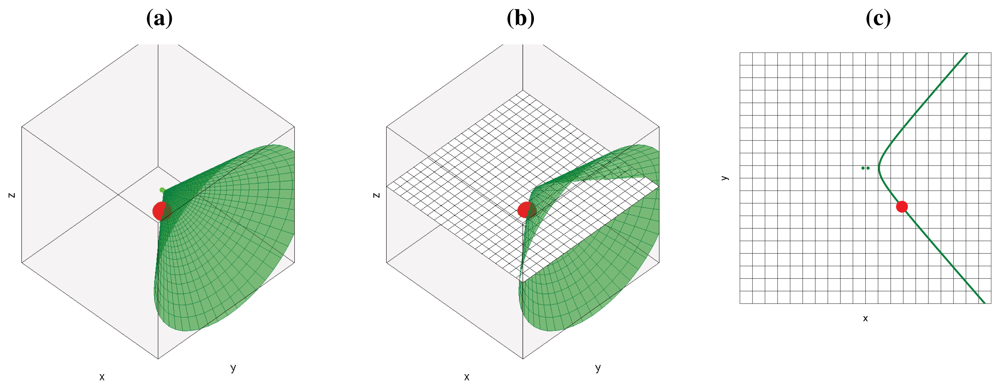
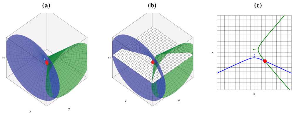
If we add additional microphone pairs, each of them will generate a new hyperboloid/hyperbola, all passing through the geometric location of the active acoustic source, as shown in Figure 2(a) for the 3D case and Figure 2(c) for the 2D case (cutting the hyperboloids by a plane as shown in Figure 2(b)). Using additional microphone pairs will allow us to disambiguate the actual position of the acoustic source, searching in the intersection of all hyperboloids/hyperbolas.
The final conclusion of this section is that, given some simplifications, for every active acoustic source and every microphone pair, we will see hyperbolic regions of constant acoustic power values in the acoustic power map generated by the ideal SRP-PHAT estimations. All the contributions for every acoustic source and every microphone pair will sum up to build the complete acoustic power map for the given situation.
3.3. Considerations in Real-World Scenarios
The simplifications established in this discussion (namely, only one omnidirectional acoustic active source, an ideal directivity pattern for the acoustic sensor array, and a non-reverberant environment) are far from being admissible in a real world scenario and deserve an additional comment:
Non-omnidirectionality of the acoustic active source: Previous studies such as [40] and [41] show that human speakers do not radiate speech uniformly in all directions. The impact of this assumption in our SRP-PHAT interpretation would lead to hyperbolic regions with different power estimations, but this effect is also present in the current formulation, as the distance between the acoustic source and the microphone varies with the source position. The use of the PHAT transform that whitens the correlation of the input signals alleviates this problem, as the module is not taken into account.
Reverberant environments: If the localization system operates in a reverberant environment, new hyperbolic regions, not initially predicted by just the position of the acoustic source, will appear. Room acoustic simulation techniques could help in improving the ability to also take into account these regions [42,43]. These false active regions actually complicate the accurate location estimation, but the problem is alleviated as more microphone pairs are taken into account: locations that are not consistent for all microphone pairs will tend to attenuate. As we will see in Section 5, our proposal is actually efficient in denoising the original SRP-PHAT power map, thus leading to better results.
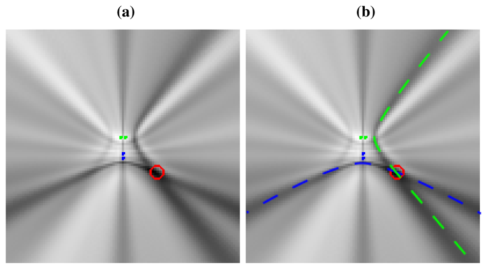
Non-ideal directivity patterns: The microphone array geometry has a profound impact in the estimation of the cross-correlation functions, as the steered response will perceive energy coming from locations different from the actual acoustic source [44]. This implies that the acoustic power map will not be composed of plain hyperboloids/hyperbolas, but of hyperbolic regions spreading from the ideal hyperbolic trajectories, as will be shown in Figure 3(a), described in the next section. There are additional considerations that contribute to this spreading effect, related to the fact that the spatial uncertainty in the correlation evaluation increases as we move further from the microphone pairs. This will be addressed also in the next section.
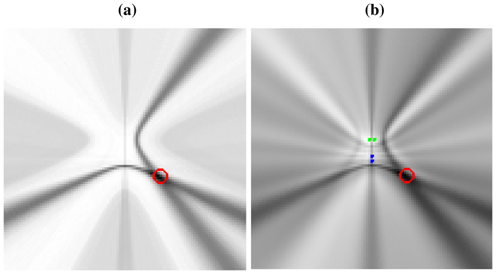
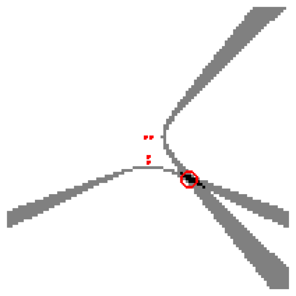
To give a real world example, Figure 3(a) shows a real SRP-PHAT image generated by two microphone pairs (blue and green dots in the center of the image) and a single active speaker located at the red circle (the higher the power, the darker the color in the map). Analyzing this image, we can clearly see two high energy, intersecting hyperbolic areas passing trough the speaker location, each one corresponding to each microphone pair. Obviously, the speaker's position corresponds to the place where those hyperbolic areas intersect, as the maximum of the power map is found at this intersection. In general, the higher the number of microphone pairs used, the better the localization performance, as more hyperbolic regions contribute to the power map estimation. In Figure 3(b) the ideal hyperbolas corresponding to each of the microphone pairs have been superimposed to the SRP-PHAT map. The power map has been calculated at a plane located 61 cm above the microphone locations, which is why the hyperbolas do not pass between the hyperbola's foci—the microphone locations.
This example shows us that in real acoustic power maps, the ideal hyperbolic functions are spread out and blurred, leading to these hyperbolic areas, and that additional hyperbolic areas appear, not explainable by just the position of the active acoustic source.
Summarizing, all these non-idealities will generate additional artifacts, additional hyperbolic regions and variations on the standard behavior of these regions in the acoustic power map that are not predicted by the ideal formulation. These non-idealities should be taken into account if we want our model to be as precise as possible. Our thesis is that our proposal, even when no developing a fully realistic model, is powerful enough to extract relevant information given realistic data, as will be shown in Section 5.
3.4. Proposal of a SRP-PHAT Based Generative Model
Taking into account the previous discussion and results, this section proposes a generative model that is able to explain the acoustic power map generated by SRP-PHAT as a sum of basis functions.
Let us define the set of scalar functions = {f(si, pj, qk)}, ┬si ∈ Q, ┬pj ∈ P, with f: ℝ3×6×3 →ℝ. From this, the general formulation of the proposal can be written as:
The basis functions f(si, pj, qk) must be designed so that they provide accurate estimations of the behavior of the real SRP-PHAT value at location qk, taking into account that there is an active source at position si and that the signal is acquired by the microphone pair pj. This generic formulation allows for models (basis functions) as complex as required, in principle able to include any of the considerations described in Section 3.3.
In the experimental work described in Section 5, we are using a relatively simple model that is able to clearly outperform standard SRP-PHAT results. In our experiments, the basis functions f(si, pj, qk) describe if point qk belongs to the hyperbolic region generated by an acoustic source sj and a given pair of microphones pj:
The model described by Equations (9) and (10) is valid to reproduce SRP-PHAT measurements, as the hyperbolic regions of the power maps are related to the high values of the Generalized Cross Correlation function of each pair of microphones [9]. Consequently the position of the hyperbolic regions is consistent with the time difference of arrival for each microphone pair given a certain speaker position.
3.5. Description of a Linear Model of SRP-PHAT
Using the model previously proposed in Equation (9) over all positions inside Q the following vector ŷ is defined:
For each position q ∈ Q, define the following vector v(s):
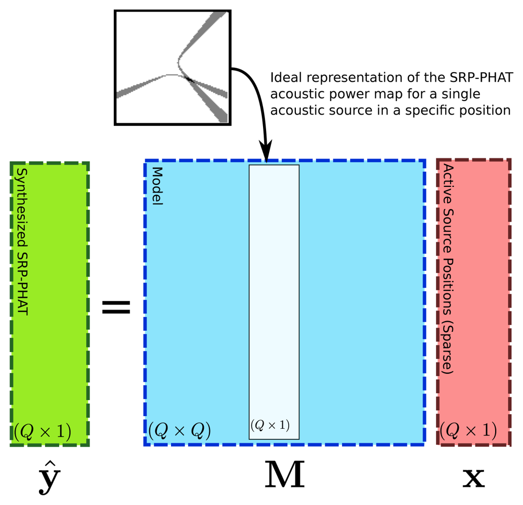
Vector v(s) can be intuitively seen as the ideal SRP-PHAT measurements that would be obtained for a single acoustic source located at position s. If Q contains points with constant height, v(s) can be visualized as an image, composed as the sum of hyperbolic areas (one for each pair of microphones), intersecting at point s (see Figure 4). It must be remarked that v is normalized by definition, i.e., max(v(s)) = 1.
The proposed generative model consists of the following linear system:
Matrix M is a Q × Q matrix whose columns are obtained using vector v defined at every s ∈ Q. Vector ŷ can be seen as the SRP-PHAT data synthesized by the proposed model as a function of weight vector x. Figure 5 shows a graphical diagram of the proposed linear model.
Expanding the terms in Equation (13), vector ŷ is obtained as the following weighted sum of vectors:
4. Model Fitting
This section explains how to use the linear model proposed in the previous section to fit real SRP-PHAT data. One of the main contribution of the paper is to show that as a result of model fitting, the performance of SRP-PHAT based localization techniques can be remarkably improved.
Suppose that vector y contains SRP-PHAT measurements (arranged in a column vector) obtained in a real scenario:
Our aim is finding a vector x capable of explaining y using model M. It is expected that y includes modeling errors, reverberation, array directivity effects, and noise, thus making the proposed model invalid for an exact representation of y. Instead, the goal will be finding a vector x capable to better explain y. The notion of which vector x is better at modeling y can be answered using optimization techniques.
The basic approach is then to solve the following optimization problem:
The approach of this paper, and one of the basis of our contribution, is to include additional constraints into Equation (17) able to give meaningful answers for x with noisy measurements, and for relatively simple basis functions in the generative model. Two basic improvements of problem (17) are proposed and detailed next.
4.1. Adding Sparse Constraints
In this paper it is assumed that there is only a small number of simultaneous active acoustic sources inside the space defined by Q, which is a reasonable assumption in the majority of scenarios considered. Given that values of x represent positions in which there is an active acoustic source, it is thus sensible to force x to have as many zeroes as possible. In the mathematical language that means to force the vector x to be a sparse vector, in which the number of non-zero elements is limited. In the optimization scheme, making the x vector to be as sparse as possible is equivalent to forcing the l0 norm of x to be minimum.
Finding the vector x that simultaneously reduces the error between the input data and the model and forces x to be as sparse as possible can be mathematically expressed as follows:
Sparse optimization methods have received remarkable attention from the scientific community. Despite its theoretical complexity, several methods and approximations have been proposed so far, and of special relevance are those methods based on using the l1 norm as a convex relaxation of the l0 norm [33,46]. This relaxation transforms (18) into the following:
Both Equations (19) and (20) are equivalent convex problems, in which convergence is guaranteed and can be solved in polynomial time.
The problem of finding a least squares estimation subject to a l1 restriction has been independently presented and popularized under the names of Least Absolute Shrinkage Selection Operator (LASSO) [47] and Basis Pursuit Denoising [32], being object of intensive study. In the past few years numerous optimization methods have been proposed, some of them adapted to specific problems.
Additionally, several generic libraries and toolboxes implementing those methods have been developed and are being extensively used. The results shown in the paper have been generated using one of these libraries [48], using a truncated Newton interior-point method, described in [49].
Solving the relaxed problem (20) does not necessary imply finding the solution to the original l0 problem. The closeness and validity of l1 relaxations have been extensively studied [33]. In some problems, the structure of matrix M and the expected degree of sparsity in the solution can make l1 relaxations to be exact. For general linear systems, as it is the case in this paper, where matrix M has no apparent structure, l1 relaxation empirically tends to impose only approximate sparse solutions. This paper provides strong experimental evidence of the improvements obtained by imposing l1 penalties, effectively making the solution x more sparse. Sparsity is a strong “prior” that helps to bias the solution x so that the effect of noise and model mismatches are properly attenuated.
4.2. Adding Subspace Filtering
Although sparsity is a well founded constraint and the l1 relaxations are effective, the experimental results in Section 5 show that, given the current model, sparsity is not strong enough to cope with errors and model mismatches in real SRP-PHAT measurements so that additional strategies must be used to improve model fitting.
This section introduces a new constraint on the problem based on filtering out the part of the input signal y that is not reproducible using model M.
First decompose y into two parts:
First, matrix M is expressed using singular value decomposition (SVD) as follows:
By identifying the number of zero singular values of M, namely Nz, the SVD decomposition shown in Equation (22) can be expressed using the following sub-matrices:
U1 and U0 are subspace projection matrices. Any nonzero vector z such that is a vector that cannot be obtained using the model M, i.e., z ≠ Mx for any possible x.
So, recalling that U*U = UU* = I, both sides of the equality (21) can be multiplied by U* with the following result:
Therefore, in order to remove the dependence of ỹ, only the Mahalanobis distance of the upper part of system (24) is optimized, regularized with the l1 term, and resulting into the problem (20) to become:
After setting to zero all the singular values below threshold ψ, we can build new matrices U′0 and , U′1 and and , for which the SVD decomposition (23) becomes:
4.3. Improving SRP-PHAT with Model Fitting
The main objective of the paper is to show that, as a result of the optimization methods proposed before, the solution x can be used to improve source localization, comparing with traditional approaches directly using SRP-PHAT measurements. The detection of local maxima in SRP-PHAT acoustic power maps is the standard way to retrieve the position of the acoustic source. This technique yields good results but is still prone to errors due to reverberation and noise and when the number of microphones is limited.
Our approach consists of replacing the original SRP-PHAT measurements y with those generated by the model solving the optimization (29), i.e., ŷ′ = M′x′, where M′ is obtained from Equation (28) and x′ is the solution of Equation (29). Vector ŷ′ can also be interpreted as a filtered/denoised version of y that is consistent with the proposed model. Figure 6 shows the acoustic power map described by the denoised vector ŷ′ (Figure 6(a)) and the original SRP-PHAT acoustic power map y (Figure 6(b)). From the figure, it seems clear that the denoising effectively reduces the number of artifacts and unwanted effects exhibited by the original map, and the assumption is that this denoised version ŷ′, if properly constrained during the optimization, is a better place to find local maxima truly representing active acoustic sources. In Section 5 the paper gives strong experimental indicators to support this idea.
5. Experiments and Discussion
5.1. Experimental Setup
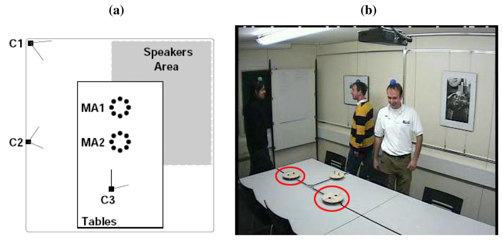
We have evaluated our proposal using the audio recordings of the AV16.3 database [50], an audio-visual corpus recorded in the Smart Meeting Room of the IDIAP research institute, in Switzerland.
The IDIAP Meeting Room consists on a 8.2 m × 3.6 m × 2.4 m rectangular room containing a centrally located 4.8 m × 1.2 m rectangular table, on top of which two circular microphone arrays of 0.1 m radius are located, each composed by 8 microphones. The centers of the two arrays are separated by 0.8 m and the origin of coordinates is located in the middle point between the two arrays. Possible speakers' locations are distributed along a L-shaped area around the table as seen in Figure 7(a). A detailed description of the meeting room can be found in [51].
The audio recordings are synchronously sampled at 16 KHz, and the complete database along with the corresponding annotation files containing the recordings ground truth is fully accessible on-line at [52]. It is composed by several sequences or recordings which range in the number of speakers involved and their activity. In this paper we will just focus on the single static speakers sequences, whose main characteristics are shown in Table 1. We will refer to the sequences as seq01, seq02 and seq03 for brevity.
Every audio sequence is assigned a corresponding annotation file containing the real ground truth positions (3D coordinates) of the speaker's mouth at every time frame in which that speaker was talking. The segmentation of acoustic frames with speech activity was first checked manually at certain time instances by a human operator in order to ensure its correctness, and later extended to cover the rest of recording time by means of interpolation techniques. The frame shift resolution was defined to be 40 ms.
5.2. Evaluation Metrics
Our localization algorithm yields a set of spatial coordinates q(t) = (x, y, z)┬ that are estimations of the actual speaker position, for every time frame t. These position estimates will be compared, by means of the Euclidean distance, to the ones labeled in a transcription file containing the real positions s(t) (ground truth), of the speaker.
We have decided to use the metrics developed under the CHIL project and described in their Evaluation Plan [53]. A complete description of the CHIL Evaluation strategies can be found at [53], but in this work we will only refer to the Multiple Object Tracking Precision (MOTP), calculated as the average localization error for all (NT) acoustically active frames in the data set: .
5.3. Evaluation Plan
We are evaluating our model in a 2D scenario, considering the acoustic power maps generated by SRP-PHAT at locations Q belonging to a plane 61 cm above the microphone array positions (this height roughly corresponds to the average height of the speaker positions in the AV16.3 sequences). Locations for SRP-PHAT data are calculated uniformly sampling Q in a 10 cm × 10 cm grid.
The procedure to generate the position estimations q(t) consists of searching for maximum values in vector ŷ′ (calculated as described in Section 4.3) that could be seen as a denoised version of the original SRP-PHAT acoustic power map.
In the experimental results shown below, we are assessing the performance of our proposal in terms of:
Optimization parameters: We will provide results depending on the two main tunable parameters of the optimization algorithms used, namely λ and eψ.
The estimation of the optimal values for this parameters will be done on an independent data set (training set) and applied to unseen data in the evaluation stage (test set).
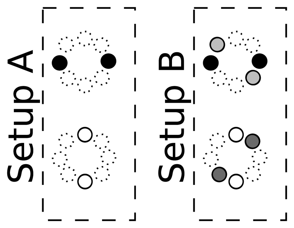
Sensor array configuration: In this work, we are using a simple microphone array configuration, aimed at evaluating our proposal in a resource-restricted environment. In order to do so, we are using 4 or 8 microphones (out of the 16 available in the AV16.3 data set), grouped in two or four microphone pairs to generate the baseline SRP-PHAT acoustic maps. The selected microphone pairs configurations are shown in Figure 8, in which microphones with the same color are considered as belonging to the same microphone pair. Given that the microphone separation for each microphone pair is 20 cm, we will violate spatial aliasing requirements, considering the signal bandwidth. Fortunately, when using SRP-PHAT, the use of more than one microphone pair alleviates this problem, as side lobes are different for each pair, and thus their effects are partially compensated.
Acoustic frame size: We will provide results depending on the length of the acoustic frame, for 80, 160 and 320 ms, to precisely assess to what extent the improvements are consistent with varying acoustic time resolutions.
The baseline we are comparing with will be the results of directly searching the maximum of the SRP-PHAT acoustic power map. The position of this maximum will correspond to the most probable source location.
Comparisons will specifically consider the relative improvement in MOTP, defined as .
Our main interest is assessing whether the results and improvements are consistent across different conditions. After describing the baseline results (in Section 5.4) and in order to evaluate the generalization capability of the proposed methods, we will address an initial study using sequence seq01 as the training set (in Section 5.5). From this study, we will decide on the optimal values of the tunable parameters used in the optimization process (those leading to the best results), and then use them to provide final performance and improvement results on the test sets, namely seq02 and seq03 (in Section 5.6). This evaluation plan ensures adequate independence and variability between train and test sets, with different speakers in all sequences (also differing in gender and height).
In all cases were appropriate, we will include references to statistical confidence values for a 95% confidence level, to adequately assess whether the improvements are statistically significant.
5.4. Baseline Results
Tables 2 and 3 show the baseline results using the standard SRP-PHAT algorithm for all sequences and different frame sizes, and the two microphone setups of Figure 8.
The main conclusions for the baseline results are:
The performance obtained is reasonable if we take into account that only two or four microphone pairs are used. Best MOTP values are around 50 cm.
Performance improves as the frame size increases, as expected, given that longer frames lead to better estimations of the correlation functions.
Adding an additional microphone pair in setup B as compared with setup A also leads to performance improvements as expected.
5.5. Evaluation of the Sensitivity to λ and eψ Values
The proposed model fitting strategies heavily depend on the estimation of adequate values for both λ and eψ (as they are the parameters controlling the optimization process), so that a detailed study on the sensitivity of the performance with variations in these parameter values is mandatory
λ expresses the relative importance of the sparse constraints applied in the optimization problems (20), (25) and (29), so that the higher its value becomes, the sparser the solution will be. In the l1 optimization software used [48], it is required that λ < λmax being λmax dependent on both the model and the input data [49]. In the results shown, the hyperparameter is represented normalized with respect to the calculated λmax: λnorm = λ/λmax, as described in [49].
The energy threshold eψ used in the subspace filtering strategy described by Equation (27) decides the size of the model that is not able to adequately explain the input signal.
To decide on the optimal λnorm and eψ to be used, we will select the values that achieve the best result in terms of MOTP, for every microphone setup and frame size.
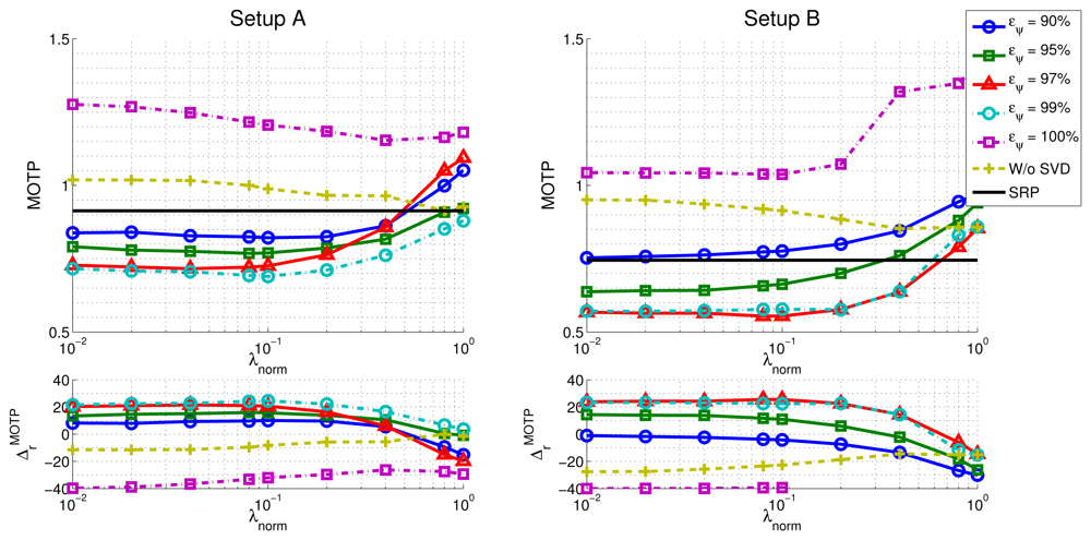
In the upper part of Figure 9, we show the evolution of the MOTP quality metric as a function of λnorm and the energy value eψ, for both microphone setups, evaluating the training sequence seq01, with a frame size of 160 ms, as an example. The horizontal black trace show the baseline results for the SRP-PHAT algorithm (obviously independent of λnorm and eψ,). In the lower part of Figure 9 the evolution of the relative improvements in MOTP are shown.
Additionally, and in order to evaluate the effectiveness of the subspace filtering step, we ran an experiment in which only the optimization with sparse constraints described in Equation (20) is applied (i.e., our proposal without using subspace filtering). The results are shown in the “W/o SVD” trace of Figure 9.
In Figure 10 we show the best MOTP results for sequence seq01 for both microphone setups and all frame sizes, with 95% confidence intervals. Data includes results for the baseline SRP-PHAT results (“SRP” in the legend, blue bars), for our proposal (“Proposal” in the legend, yellow bars), and for our proposal without applying the SVD step (“Proposal w/o SVD” in the legend, green bars) (the orange bar (“SVD+SRP” in the legend) refers to results that will be discussed later).
From this, we can conclude that, for adequate values of the optimization tuning parameters:
Our proposal is able to improve the SRP-PHAT results with statistically significant relative improvements of up to almost 25%, with consistent improvements for a wide range of λnorm values.
Microphone setups have a similar impact in the relative performance improvements. The improvements for setups A and B are 24.6% and 25.6%, respectively.
In what respect to the dependency of the best results with λnorm (once selected the optimal eψ), both microphone setups show a desirable behavior, achieving a reasonably clear optimal area for a wide range of parameter values.
Using either the model with sparse constraints (i.e., “Proposal w/o SVD”) or SVD without actually filtering (i.e., eψ = 100%) is giving worse localization results than the SRP-PHAT baseline algorithm. It thus seems that fitting the complete model to data is not making any progress even if sparse constraints are included. The explanation of this phenomenon was partially advanced in Section 4.2 but it needs some additional justification. The model that is proposed in this paper is not able to explain every SRP-PHAT map (i.e., matrix M is rank-deficient). When using any of the optimization strategies proposed in the paper, the position of speakers is the result of looking at local maxima in the SRP-PHAT map reproduced through the model. Therefore, in theory, the results must not be necessarily equal to the baseline algorithm, even if subspace filtering is removed, or the l1 term is not having strong influence. Empirical data tell us that in these cases, localization results can be in fact worse than the baseline. The main result of the paper is to show through experiments that statistically significant improvements can be reached using a specific combination of subspace filtering and sparse constraints. In these cases the model is able to adequately filter the effects of noise and reverberation in the SRP-PHAT map, giving a cleaner image about the real position of the speaker.
Interestingly, the optimal values for the parameters controlling the optimization process are identical for all frame sizes in the setup A . This seems not to be the case for setup B, in which in all cases, but values varies for different frame sizes. However, even in this case, the improvements are stable for a wide range of parameter values as can be seen in the first three rows of Table 5, where the relative improvements have been calculated for different values of λnorm (0.04, 0.08 and 0.1), setting .
From Table 4 it also seems that the optimal values of the parameters are dependent on the microphone setup used, as both and are different for setups A and B. A more detailed evaluation shows that, again, the improvements are stable even when we use the optimal values estimated for setup A , in the optimization process for setup B data, as it can be seen in the last row of Table 5.
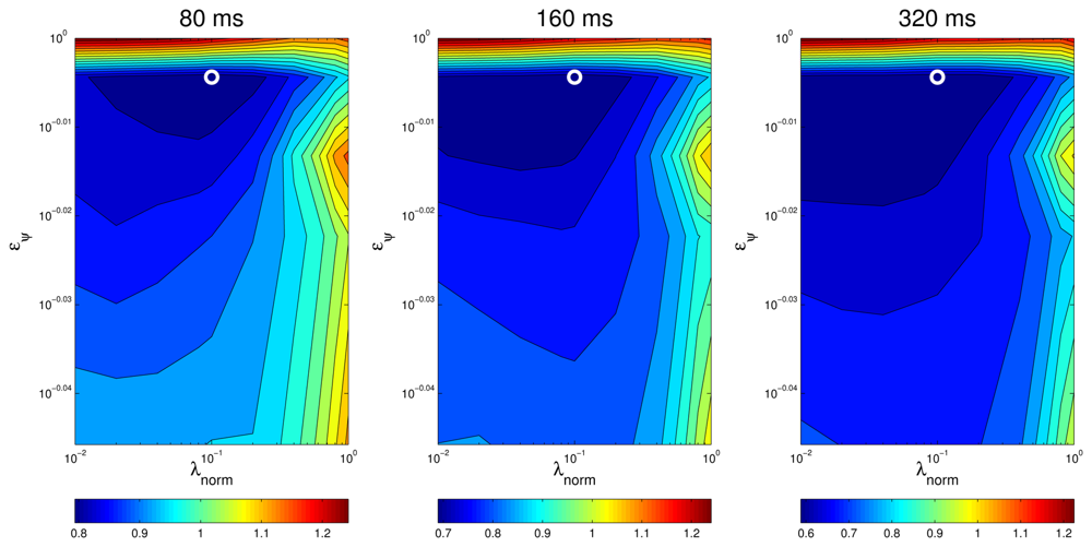
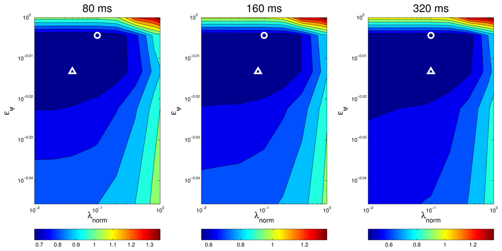
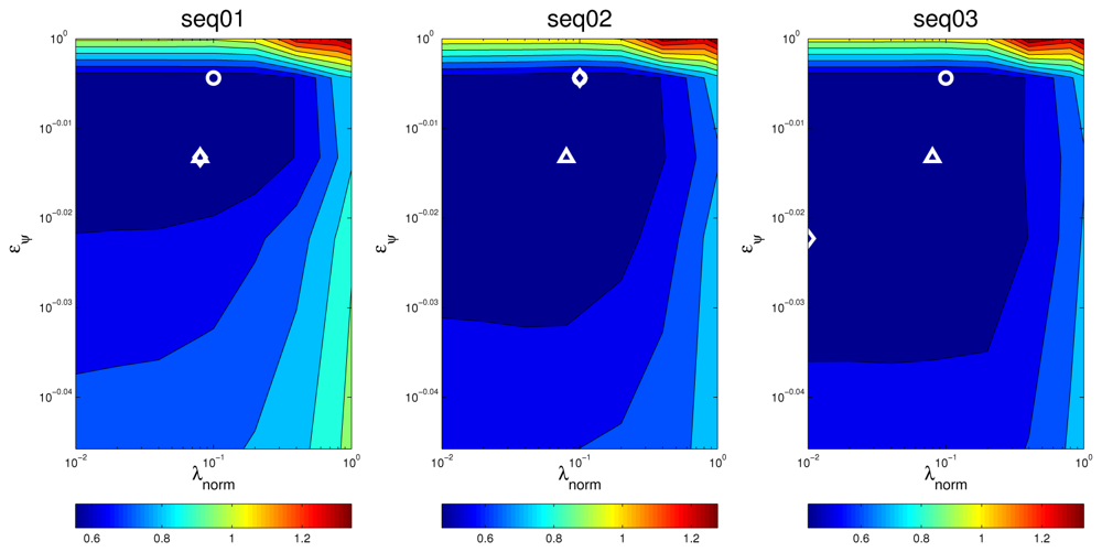
An additional way of visually assessing to what extent the results of the optimal values for the optimization parameters are consistent for different situations is plotting a surface map of MOTP versus variations on λnorm and eψ and making a comparison. For example, Figures 11 and 12 show this optimization map for microphone setups A and B respectively, using sequence seq01. In these maps, the optimal points for each evaluation are represented with a circle for seq01 and setup A, and with a triangle for seq01 and setup A. The maps show a similar structure for the optimal region in both microphone setups, supporting the idea that the optimal optimization parameters do not heavily depend on changes of the experimental conditions. Moreover, in the cases for microphone setup B, where the optimal points (triangles) seem not to be close to the optimal points of setup A (circles), it can be seen that these positions belong to an area with roughly the same MOTP level (the area can be recognized as a flat optimal region).
The main conclusion of these experiments is that, for the given experimental setup, our proposal is able to clearly outperform the standard SRP-PHAT results. The statistically significant relative improvements roughly vary between 22% and 30%, and, what is more important, with little sensitivity to the optimization parameters selected when changing the microphone setup and the frame size used (once the optimal parameters have been estimated for the training data).
To further evaluate the contribution of the subspace filtering strategy, we ran an experiment in which we applied the subspace filtering to the original SRP-PHAT data, that is, projecting the SRP-PHAT acoustic power map on the span of model M′ obtained from (28). This projection generates a new filtered power map, calculated as . The results applying this transformation are given in the orange bars of Figures 10 and 15, referred to as “SVD+SRP”. In these figures, we can see that SRP+SVD also outperforms SRP, although the differences are not statistically significant.
5.6. Evaluation on the Test Set
The evaluation carried out in the previous section only addresses the estimation of the optimal parameters for a single training sequence and the proposal evaluation on this same data set (seq01). We still need to assess whether the optimal values estimated for the training data set are able to achieve good results when using different sequences. As stated above, we are using seq02 and seq03 as independent test sets.
Figures 13 and 14 show the optimization maps for all sequences, frame size 160 ms, and microphone setups A and B, respectively. The cross is located in the optimal point for each sequence and setup A, and the diamond is located in the optimal point for each sequence and setup B. It can be seen that, again, the structure of the optimal regions are reasonably similar, thus suggesting that the optimal values for the optimization parameters estimated in the training set will also achieve good results in the test sets. The position of the optimal points in each map also belong to the same flat optimal region.
Figure 15 shows the best MOTP results for sequences seq02 and seq03 for both microphone setups and all frame sizes, with 95% confidence intervals (using the optimal parameter values estimated for the training sequence seq01).
Tables 6 and 7 show the relative improvements achieved when evaluating sequences seq02 and seq03 for both microphone setups, also using the optimal parameter values for sequence seq01. As expected, the relative improvements are in the range of those obtained for sequence seq01, except for sequence seq02 and microphone setup A (with lower improvements of around 10%). Our hypothesis is that the fact that this is a female speaker imposes significant differences in the speech signals, thus modifying the correlation functions used in the input data, and posing additional difficulties to the optimization process when only two microphone pairs are used. Nevertheless, this will have to be evaluated in future work.
Apart from the case of seq02 with setup A, the improvements are relevant and statistically significant, roughly varying between 20% and 30%. These achievements also show little sensitivity to the optimization parameters selected, in spite of the fact that we are additionally dealing with different speakers.
6. Conclusions and Future Work
This paper has proposed a novel method to localize active acoustic sources in a room equipped with sensor arrays. Two main contributions can be highlighted: First, a simple but very promising generative linear model is proposed to explain SRP-PHAT data taken from any geometrical combination of microphone arrays. The model simply reflects the geometry of three-dimensional points sharing common difference of time-of-arrival between each microphone pair. This model is independent of the spectrum properties of the signals emitted by the source and can be easily computed in practice. Second, this paper shows, using convincing experiments based on publicly available data, that such a simple model can be used to fit real SRP-PHAT data that is usually very noisy and has many unmodeled effects (such as reverberation in the scene). Fitting the model is done by imposing two constraints. The first one is forcing the model parameters to be sparse, as acoustic sources cannot be densely distributed in a typical environment. The second constraint simply removes the part of the measurements that is not exactly reproducible by the model. In the light of the experimental results, these two constraints in combination are the real key of the paper, notably improving the performance of state-of-the-art localization methods based on SRP-PHAT. It is also worth mentioning that all algorithms and experiments proposed in the paper are very easy to reproduce.
In future works the performance of this approach must be thoroughly validated in rooms with multiple speakers and using the whole three-dimensional set of spatial positions. Immediate improvements should cover all issues commented in Section 3.3. That means to propose basis functions in the model that take into account additional factors, such as the spectral content of the acoustic sources, directivity pattern effects in the microphone arrays, and also adding geometric information that would help to predict reverberation effects. The authors believe that improvements in the model may yield remarkable improvements in the localization accuracy in real world scenarios.
Acknowledgments
This work has been supported by the Spanish Ministry of Science and Innovation under projects VISNU (ref. TIN2009-08984) and SDTEAM-UAH (ref. TIN2008-06856-C05-05). We also thank the anonymous reviewers for their constructive feedback and helpful suggestions.
References
- Weiser, M. Some computer science issues in ubiquitous computing. Commun. ACM 1993, 36, 75–84. [Google Scholar]
- Pentland, A. Smart rooms. Sci. Am. 1996, 274, 54–62. [Google Scholar]
- Lee, J.; Hashimoto, H. Intelligent space concept and contents. Adv. Robot. 2002, 16, 265–280. [Google Scholar]
- Fleuret, F.; Berclaz, J.; Lengagne, R.; Fua, P. Multicamera people tracking with a probabilistic occupancy map. IEEE Trans. Pattern Anal. Mach. Intell. 2008, 30, 267–282. [Google Scholar]
- Marron-Romera, M.; Garcia, J.; Sotelo, M.; Pizarro, D.; Mazo, M.; Cañas, J.; Losada, C.; Marcos, A. Stereo vision tracking of multiple objects in complex indoor environments. Sensors 2010, 10, 8865–8887. [Google Scholar]
- Pizarro, D.; Mazo, M.; Santiso, E.; Marron, M.; Jimenez, D.; Cobreces, S.; Losada, C. Localization of mobile robots using odometry and an external vision sensor. Sensors 2010, 10, 3655–3680. [Google Scholar]
- Lowe, D. Object recognition from local scale-invariant features. Proceedings of the Seventh IEEE International Conference on Computer Vision, Kerkyra, Greece, 20– 27 September 1999; pp. 1150–1157.
- Brandstein, M.S.; Silverman, H.F. A practical methodology for speech source localization with microphone arrays. Comput. Speech Lang. 1997, 11, 91–126. [Google Scholar]
- DiBiase, J.; Silverman, H.; Brandstein, M. Robust localization in reverberant rooms. In Microphone Arrays: Signal Processing Techniques and Applications, 1st ed.; Brandstein, M.S., Ward, D.B., Eds.; Springer-Verlag: New York, NY, USA, 2001; pp. 157–180. [Google Scholar]
- Waibel, A.; Stiefelhagen, R. Computers in the Human Interaction Loop, 2nd ed.; Springer: London, UK, 2009. [Google Scholar]
- DiBiase, J. A high-accuracy, low-latency technique for talker localization in reverberant environments using microphone arrays. Ph.D. Thesis, Brown University, Providence, RI, USA, 2000. [Google Scholar]
- Gillette, M.; Silverman, H. A Linear Closed-Form Algorithm for Source Localization from Time-Differences of Arrival. IEEE Signal Process. Lett. 2008, 15, 1–4. [Google Scholar]
- Knapp, C.; Carter, G. The generalized correlation method for estimation of time delay. IEEE Trans. Acoust. Speech Signal Process 1976, 24, 320–327. [Google Scholar]
- Zhang, C.; Florencio, D.; Zhang, Z. Why does PHAT work well in low noise, reverberative environments? Proceedings of ICASSP 2008 on Acoustics, Speech and Signal Processing, Las Vegas, NV, USA, 31 March-4 April 2008; pp. 2565–2568.
- Dmochowski, J.P.; Benesty, J. Steered Beamforming Approaches for Acoustic Source Localization. In Speech Processing in Modern Communication, 1st ed.; Cohen, I., Benesty, J., Gannot, S., Eds.; Springer-Verlag: Berlin/Heidelberg, Germany, 2010; Volume 3, pp. 307–337. [Google Scholar]
- Omologo, M.; Svaizer, P. Use of The Cross-Power-Spectrum Phase in Acoustic Event Location. IEEE Trans. Speech Audio Process 1993, 5, 288–292. [Google Scholar]
- Dmochowski, J.; Benesty, J.; Affes, S. A Generalized Steered Response Power Method for Computationally Viable Source Localization. IEEE Trans. Speech Audio Process 2007, 15, 2510–2526. [Google Scholar]
- Badali, A.; Valin, J.M.; Michaud, F.; Aarabi, P. Evaluating real-time audio localization algorithms for artificial audition in robotics. Proceedings of IEEE /RSJ International Conference on Intelligent Robots and Systems, St. Louis, MO, USA, 10– 15 October 2009; pp. 2033–2038.
- Do, H.; Silverman, H. SRP-PHAT methods of locating simultaneous multiple talkers using a frame of microphone array data. Proceedings of 2010 IEEE International Conference on Acoustics Speech and Signal Processing, Dallas, TX, USA, 14– 19 March 2010; pp. 125–128.
- Cobos, M.; Marti, A.; Lopez, J. A modified SRP-PHAT functional for robust real-time sound source localization with scalable spatial sampling. IEEE Signal Proc. Lett. 2011, 18, 71–74. [Google Scholar]
- Butko, T.; Gonzalez Pla, R.; Segura Perales, C.; Nadeu Camprubí, C.; Hernando Pericás, F.J. Two-source acoustic event detection and localization: Online implementation in a smart-room. Proceedings of the 17th European Signal Processing Conference (EUSIPCO'11), Barcelona, Spain, 29 August-2 September 2011; pp. 1317–1321.
- Habets, E.A.P.; Benesty, J.; Gannot, S.; Cohen, I. The MVDR Beamformer for Speech Enhancement. In Speech Processing in Modern Communication; Cohen, I., Benesty, J., Gannot, S., Eds.; Springer: Berlin/Heidelberg, Germany, 2010; Volume 3; pp. 225–254. [Google Scholar]
- Zhang, C.; Zhang, Z.; Florencio, D. Maximum Likelihood Sound Source Localization for Multiple Directional Microphones. Proceedings of IEEE International Conference on Acoustics, Speech and Signal Processing, Honolulu, HI, USA, 15– 20 April 2007; Volume 1. pp. I-125–I-128.
- Zhang, C.; Florencio, D.; Ba, D.; Zhang, Z. Maximum Likelihood Sound Source Localization and Beamforming for Directional Microphone Arrays in Distributed Meetings. IEEE Trans. Multimed. 2008, 10, 538–548. [Google Scholar]
- Schmidt, R. Multiple emitter location and signal parameter estimation. IEEE Trans. Antenn. Propag. 1986, 34, 276–280. [Google Scholar]
- Baraniuk, R. Compressive sensing [lecture notes]. IEEE Signal Process. Mag. 2007, 24, 118–121. [Google Scholar]
- Candes, E. The restricted isometry property and its implications for compressed sensing. C R. Math. 2008, 346, 589–592. [Google Scholar]
- Rao, B.; Kreutz-Delgado, K. An affine scaling methodology for best basis selection. IEEE Trans. Signal Process 1999, 47, 187–200. [Google Scholar]
- Davis, G.; Mallat, S.; Avellaneda, M. Adaptive greedy approximations. Constr. Approx. 1997, 13, 57–98. [Google Scholar]
- Temlyakov, V. Nonlinear methods of approximation. Found. Comput. Math. 2003, 3, 33–107. [Google Scholar]
- Tropp, J. Greed is good: Algorithmic results for sparse approximation. IEEE Trans. Inform. Theor. 2004, 50, 2231–2242. [Google Scholar]
- Chen, S.; Donoho, D.; Saunders, M. Atomic decomposition by basis pursuit. SIAM Rev. 2001, 43, 129–159. [Google Scholar]
- Tropp, J. Just relax: Convex programming methods for identifying sparse signals in noise. IEEE Trans. Inform. Theor. 2006, 52, 1030–1051. [Google Scholar]
- Claerbout, J.; Muir, F. Robust modeling with erratic data. Geophysics 1973, 38, 826. [Google Scholar]
- Malioutov, D.; Cetin, M.; Willsky, A. A sparse signal reconstruction perspective for source localization with sensor arrays. IEEE Trans. Signal Process 2005, 53, 3010–3022. [Google Scholar]
- Sun, K.; Liu, Y.; Meng, H.; Wang, X. Adaptive Sparse Representation for Source Localization with Gain/Phase Errors. Sensors 2011, 11, 4780–4793. [Google Scholar]
- Ba, D.; Ribeiro, K.; Zhang, C.; Florêncio, D. L1 regularized room modeling with compact microphone arrays. Proceedings of 2010 IEEE International Conference on Acoustics Speech and Signal Processing (ICASSP), Dallas, TX, USA, 14– 19 March 2010; pp. 157–160.
- Ribeiro, R.; Ba, D.; Zhang, C.; Floêncio, D. Turning enemies into friends: Using reflections to improve sound source localization. Proceedings of 2010 IEEE International Conference on Multimedia and Expo (ICME), Singapore, 19– 23 July 2010; pp. 731–736.
- Chardon, G.; Daudet, L. Narrowband source localization in an unknown reverberant environment using wavefield sparse decomposition. Proceedings of 2012 IEEE International Conference on Acoustics, Speech and Signal Processing (ICASSP), Kyoto, Japan, 25– 30 March 2012; pp. 9–12.
- Meuse, P.; Silverman, H. Characterization of talker radiation pattern using a microphone array. Proceedings of 1994 IEEE International Conference on Acoustics, Speech, and Signal Processing, Adelaide, Australia, 19– 22 April 1994; pp. 257–260.
- Chu, W.; Warnock, A. Detailed Directivity of Sound Fields Around Human Talkers; Research Report; Institute for Research in Construction: Ottawa, ON, Canada, 2002. [Google Scholar]
- Wabnitz, A.; Epain, N.; Jin, C.T.; van Schaik, A. Room acoustics simulation for multichannel microphone arrays. Proceedings of the International Symposium on Room Acoustics, Melbourne, Australia, 29–31 August 2010.
- Kowalczyk, K.; van Walstijn, M. Room acoustics simulation using 3-D compact explicit FDTD schemes. IEEE Trans. Audio Speech Lang. Process 2011, 19, 34–46. [Google Scholar]
- Ziomek, L.J. Fundamentals of Acoustic Field Theory and Space-Time Signal Processing; CRC Press: Boca Raton, FL, USA, 1995. [Google Scholar]
- Tikhonov, A.; Arsenin, V.; John, F. Solutions of Ill-Posed Problems; Vh Winston: Washington, DC, USA, 1977. [Google Scholar]
- Tropp, J.A. Algorithms for simultaneous sparse approximation. Part II: Convex relaxation. Signal Process 2006, 86, 589–602. [Google Scholar]
- Tibshirani, R. Regression shrinkage and selection via the lasso. J. R. Statist. Soc. B. 1996, 58, 267–288. [Google Scholar]
- Koh, K.; Kim, S.; Boyd, S. 11_1s: A Matlab Solver for Large-Scale 11-Regularized Least Squares Problems. Available online: http://www.stanford.edu/boyd/11_1s/ (accessed on 11 October 2012).
- Kim, S.; Koh, K.; Lustig, M.; Boyd, S.; Gorinevsky, D. An interior-point method for large-scale 11-regularized least squares. IEEE J. Sel. Top. Signal Process 2007, 1, 606–617. [Google Scholar]
- Lathoud, G.; Odobez, J.M.; Gatica-Perez, D. AV16.3: An Audio-Visual Corpus for Speaker Localization and Tracking. Proceedings of First International Workshop on Machine Learning for Multimodal Interaction, Martigny, Switzerland, 21–23 June 2004.
- Moore, D.C. The IDIAP Smart Meeting Room; Technical Report; IDIAP Research Institute: Martigny, Switzerland, 2004. [Google Scholar]
- Lathoud, G. AV16.3 Dataset. Available online: http://www.idiap.ch/dataset/avl6-3/ (accessed on 11 October 2012).
- Mostefa, D.; Garcia, M.; Bernardin, K.; Stiefelhagen, R.; McDonough, J.; Voit, M.; Omologo, M.; Marques, F.; Ekenel, H.; Pnevmatikakis, A. Clear Evaluation Plan, Technical Report; Document CHIL-CLEAR-V1.1. Available online: http://www.clear-evaluation.org/clear06/downloads/chil-clear-v1.l-2006-02-21.pdf (accessed on 11 October 2012).


| Sequence name | speaker | Average speaker height* (m) | duration(s) | number of ground truth frames |
|---|---|---|---|---|
| seq01-1p-0000 | male | 54.3 | 208 | 2,248 |
| seq02-1p-0000 | female | 62.5 | 171 | 2,411 |
| seq03-1p-0000 | male | 70.3 | 220 | 2,636 |
*In the reference coordinate system.
| 80 ms | 160 ms | 320 ms | ||
|---|---|---|---|---|
| seq01 | MOTP | 1.02 ± 0.03 | 0.91 ± 0.03 | 0.83 ± 0.03 |
| seq02 | MOTP | 0.96 ± 0.03 | 0.84 ± 0.03 | 0.77 ± 0.02 |
| seq03 | MOTP | 0.90 ± 0.03 | 0.77 ± 0.03 | 0.69 ± 0.03 |
| 80 ms | 160 ms | 320 ms | ||
|---|---|---|---|---|
| seq01 | MOTP | 0.87 ± 0.03 | 0.74 ± 0.03 | 0.62 ± 0.02 |
| seq02 | MOTP | 0.73 ± 0.02 | 0.62 ± 0.02 | 0.56 ± 0.02 |
| seq03 | MOTP | 0.71 ± 0.02 | 0.59 ± 0.02 | 0.50 ± 0.01 |
| 80 ms | 160 ms | 320 ms | ||
|---|---|---|---|---|
| setup A | 22.1% | 24.6% | 29.1% | |
| 0.1 | 0.1 | 0.1 | ||
| 99% | 99% | 99% | ||
| setup B | 22.9% | 25.6% | 27.6% | |
| 0.04 | 0.08 | 0.1 | ||
| 97% | 97% | 97% | ||
| 80ms | 160ms | 320ms | ||
|---|---|---|---|---|
| setup B | 22.9% | 24.2% | 26.7% | |
| λnorm | 0.04 | 0.04 | 0.04 | |
| setup B | 22.1% | 25.6% | 27.2% | |
| λnorm | 0.08 | 0.08 | 0.08 | |
| setup B | 22.2% | 25.3% | 27.6% | |
| λnorm | 0.1 | 0.1 | 0.1 | |
| setup B | 21.4% | 22.6% | 24.3% | |
| 80 ms | 160 ms | 320 ms | ||
|---|---|---|---|---|
| setup A | 10.0% | 9.6% | 9.9% | |
| λnorm | 0.1 | 0.1 | 0.1 | |
| eψ | 99% | 99% | 99% | |
| setup B | 20.7% | 22.9% | 25.1% | |
| λnorm | 0.04 | 0.08 | 0.1 | |
| eψ | 97% | 97% | 97% | |
| 80 ms | 160 ms | 320 ms | ||
|---|---|---|---|---|
| setup A | 23.8% | 26.9% | 29.9% | |
| λnorm | 0.1 | 0.1 | 0.1 | |
| eψ | 99% | 99% | 99% | |
| setup B | 25.7% | 27.3% | 29.0% | |
| λnorm | 0.04 | 0.08 | 0.1 | |
| eψ | 97% | 97% | 97% | |
© 2012 by the authors; licensee MDPI, Basel, Switzerland. This article is an open access article distributed under the terms and conditions of the Creative Commons Attribution license (http://creativecommons.org/licenses/by/3.0/).
Share and Cite
Velasco, J.; Pizarro, D.; Macias-Guarasa, J. Source Localization with Acoustic Sensor Arrays Using Generative Model Based Fitting with Sparse Constraints. Sensors 2012, 12, 13781-13812. https://doi.org/10.3390/s121013781
Velasco J, Pizarro D, Macias-Guarasa J. Source Localization with Acoustic Sensor Arrays Using Generative Model Based Fitting with Sparse Constraints. Sensors. 2012; 12(10):13781-13812. https://doi.org/10.3390/s121013781
Chicago/Turabian StyleVelasco, Jose, Daniel Pizarro, and Javier Macias-Guarasa. 2012. "Source Localization with Acoustic Sensor Arrays Using Generative Model Based Fitting with Sparse Constraints" Sensors 12, no. 10: 13781-13812. https://doi.org/10.3390/s121013781
APA StyleVelasco, J., Pizarro, D., & Macias-Guarasa, J. (2012). Source Localization with Acoustic Sensor Arrays Using Generative Model Based Fitting with Sparse Constraints. Sensors, 12(10), 13781-13812. https://doi.org/10.3390/s121013781