X-Ray Detected Magnetic Resonance: A Unique Probe of the Precession Dynamics of Orbital Magnetization Components

Abstract
:1. Introduction
 , Sj ] in which the spin Hamiltonian
was given the following form:
, Sj ] in which the spin Hamiltonian
was given the following form:- For crystal fields weak compared to spin-orbit coupling, J is a good quantum number and the crystal field simply splits the relevant manifold according to site symmetry. Ions with half-integral J’s always have a double Kramer’s degeneracy and fictitious spins take the following values:
![Ijms 12 08797f10]() = 0, 1/2, 1 or 3/2.
= 0, 1/2, 1 or 3/2. - If the crystal field is large compared to spin-orbit coupling, it splits the L-multiplet. If the lowest state is a singlet, the (quenched) orbital moment has no first order contribution. Recall that an orbitally threefold degenerate T-state mathematically is isomorphic to a P-state (L = 1): it can be described with a fictitious angular momentum
![Ijms 12 08797f11]() which, in turn, couples to the spin angular momentum to yield a fictitious-spin
which, in turn, couples to the spin angular momentum to yield a fictitious-spin
![Ijms 12 08797f10]() .
.

 = 〈Sz〉 in which ρ ≠ 1 is a constant factor. Ultimately, a fictitious magnetization vector M can be defined which satisfies the equation of motion:
 reduces to a Zeeman term for EPR spectra whereas a compact formulation of the fictitious magnetization can be given using commonly accepted tensor notations:
 = −gααμB
  with α = x, y, z. Concretely, the first or second order perturbations associated with orbital moments and spin-orbit interactions essentially affect the resonance through the spectroscopic splitting factor g which becomes a rank-2 tensor property. Recall that det [g] = gxxgyygzz determines the helicity of the precession in the resonance field H [18]. Equation 3, however, does not tell us anything clear about the precession of orbital magnetization components, in particular in excited states.
2. Resonant Precession of Spin and Orbital Magnetization Components in Excited States
2.1. Specificity of the XMCD Probe
2.2. Site-Selective Probe in Ferrimagnetic Iron Garnets
 ) and octahedral (
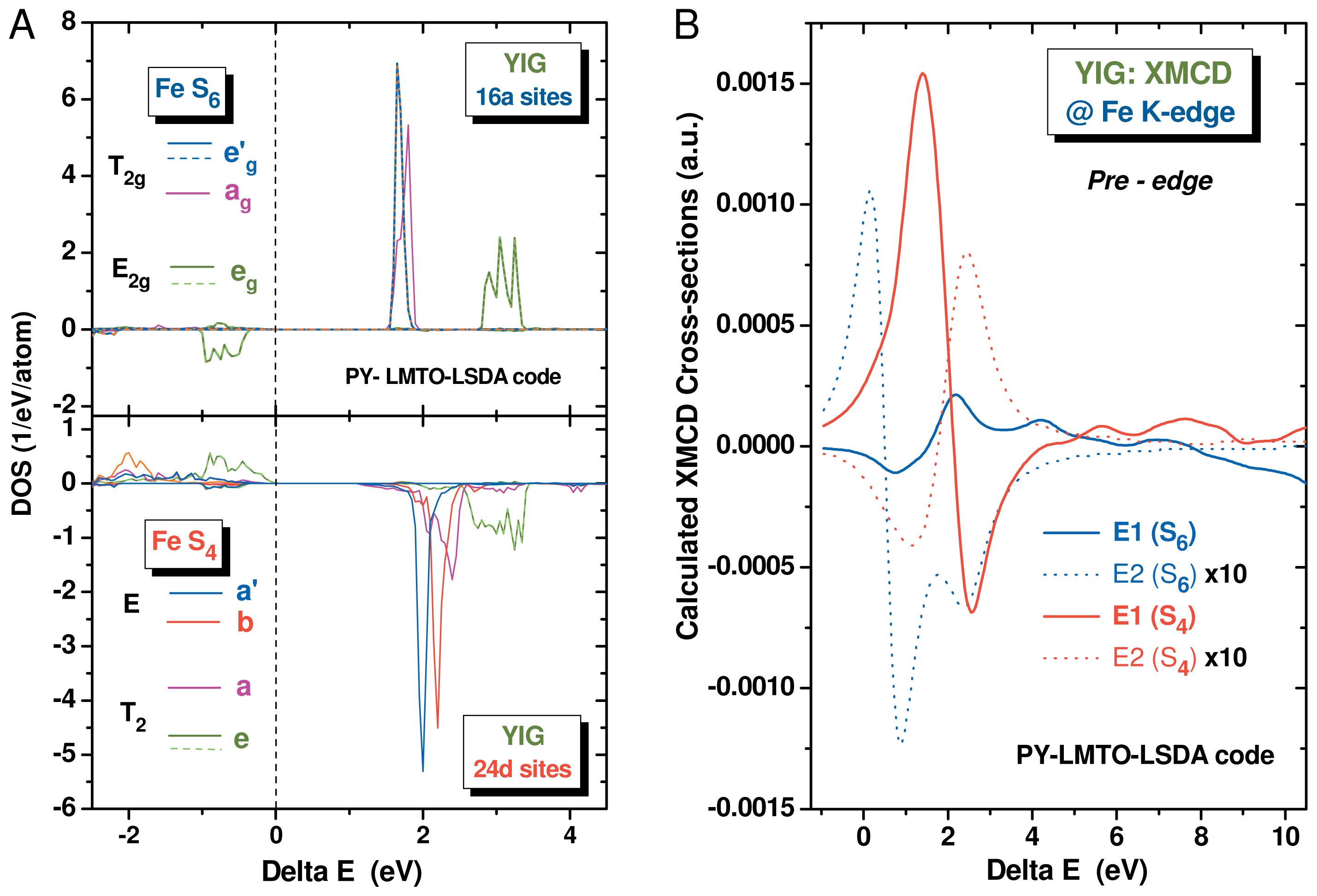
 ) coordination symmetry respectively. This is fully consistent with the antiferromagnetic coupling of the Fe ions in (24d) and (16a) sites [33]. Let us draw attention, however, onto the opposite sign of the spin polarized DOS in the filled states (ΔE < 0) and in the excited states (ΔE > 0) which belong to the same irreducible representation of groups
or
: this implies that the corresponding magnetization components should precess with the opposite helicity in the ground and excited states. as the 4p atomic orbitals. In contrast, transitions from the 1s core level to final states belonging to the ag or eg representations are allowed only by E2 transitions which have a much lower contribution to the XMCD cross-sections. In other terms, XDMR spectra recorded at the maximum intensity of the Fe K-edge XMCD spectrum will benefit from a strong site-selectivity favoring the
Fe sites: this is a considerable advantage over FMR. Recall, however, that site-selectivity is lost if the XDMR spectra are collected at the L2,3 edges of iron since 2p → 3d transitions are dipole allowed at both sites.
) coordination symmetry respectively. This is fully consistent with the antiferromagnetic coupling of the Fe ions in (24d) and (16a) sites [33]. Let us draw attention, however, onto the opposite sign of the spin polarized DOS in the filled states (ΔE < 0) and in the excited states (ΔE > 0) which belong to the same irreducible representation of groups
or
: this implies that the corresponding magnetization components should precess with the opposite helicity in the ground and excited states. as the 4p atomic orbitals. In contrast, transitions from the 1s core level to final states belonging to the ag or eg representations are allowed only by E2 transitions which have a much lower contribution to the XMCD cross-sections. In other terms, XDMR spectra recorded at the maximum intensity of the Fe K-edge XMCD spectrum will benefit from a strong site-selectivity favoring the
Fe sites: this is a considerable advantage over FMR. Recall, however, that site-selectivity is lost if the XDMR spectra are collected at the L2,3 edges of iron since 2p → 3d transitions are dipole allowed at both sites.2.3. Steady-State, Uniform Mode of Precession
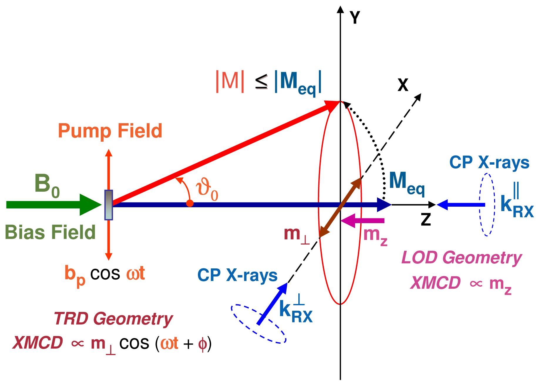
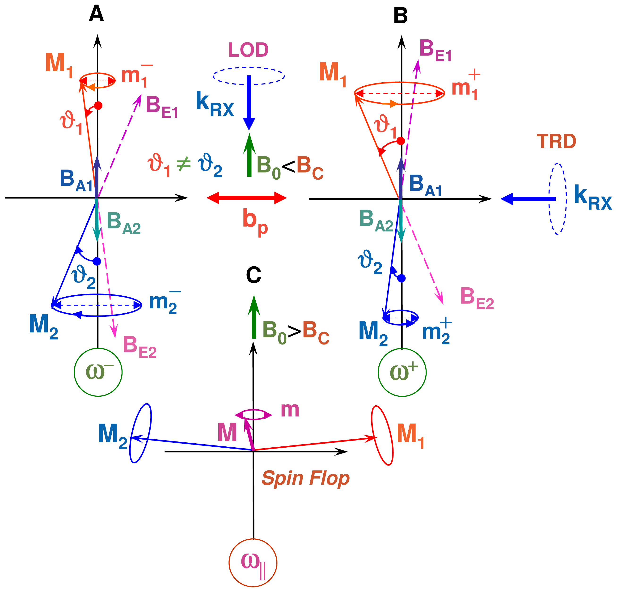
- - In the transverse geometry (TRD), the wavevector kRX⊥ of the incident, circularly polarized X-rays is set perpendicular to both the static bias field B0 and the oscillating pump field bp: the XMCD probe is then proportional to the transverse magnetization m⊥ which oscillates at microwave frequency.
- - In the longitudinal geometry (LOD), the X-ray wavevector kRX|| is set parallel to the static bias field B0. If one assumes that Ms = |Meq|, then there is a steady-state change mz of the projection of the magnetization along the Z axis and there should be a time-invariant XMCD signal ∝ mz. Unfortunately, mz is only a second order effect with respect to the opening angle of precession (θ0) and m⊥. Moreover, any information regarding the phase or helicity of the precession gets lost.
2.4. Precession Eigen Modes and Spin Waves
2.4.1. Magnetostatic Walker’s Modes
2.4.2. Exchange Spin Waves
. Usually, spin-wave excitations in ferromagnets are sufficiently small that
can be expanded in a Taylor series in powers of ck and ck*: but it corresponds to the linear theory of spin waves: it yields the energy of non-interacting modes with the dispersion law : ωk = [Ak2 – |Bk|2]1/2 in which:
 ) arises from the Zeeman interaction with the transverse field component b⊥:
 is responsible for the spin wave instability in parallel pumping [43]:
 =
=
 +
+
 with [39]: and
describe three- and four-magnon interactions respectively. Three-magnon processes, in either the confluent or splitting modes, arise not only from long range dipole-dipole interactions as first recognized by Akhiezer [40], but also from short range pseudo-dipolar interactions [14]. Energy conservation implies that: ω1 = ω2 + ω3 for a 3-magnon splitting process, whereas (ω1 + ω2) = (ω3 + ω4) in a 4-magnon scattering process. Even though
refers to a higher order perturbation, the 4-magnon scattering process is the corner stone of all nonlinear theories of spin waves [41] because exchange may largely dominate over dipole-dipole interactions in this term [39]. Given that the exchange part is α (k1 · k2)2, it immediately appears, however, that the exchange cross section is zero if either k1 or k2 is zero: in other terms, exchange cannot relax the uniform mode (k = 0). As pointed out by Keffer [39], this is consistent with the well known result (see for instance [42]) that the Heisenberg exchange Hamiltonian commutes with all vector components of the total spin operator:
with [39]: and
describe three- and four-magnon interactions respectively. Three-magnon processes, in either the confluent or splitting modes, arise not only from long range dipole-dipole interactions as first recognized by Akhiezer [40], but also from short range pseudo-dipolar interactions [14]. Energy conservation implies that: ω1 = ω2 + ω3 for a 3-magnon splitting process, whereas (ω1 + ω2) = (ω3 + ω4) in a 4-magnon scattering process. Even though
refers to a higher order perturbation, the 4-magnon scattering process is the corner stone of all nonlinear theories of spin waves [41] because exchange may largely dominate over dipole-dipole interactions in this term [39]. Given that the exchange part is α (k1 · k2)2, it immediately appears, however, that the exchange cross section is zero if either k1 or k2 is zero: in other terms, exchange cannot relax the uniform mode (k = 0). As pointed out by Keffer [39], this is consistent with the well known result (see for instance [42]) that the Heisenberg exchange Hamiltonian commutes with all vector components of the total spin operator:
 = ∑i Si so-that: [
 ,
,
 ] = [
,
] = [
,
 ] = [
,
] = [
,
 ] = 0. In particular, this implies that the Heisenberg exchange Hamiltonian should also commute with the longitudinal (z) component of the magnetization: [
,
] = 0. In particular, this implies that the Heisenberg exchange Hamiltonian should also commute with the longitudinal (z) component of the magnetization: [
,
 ] = 0.
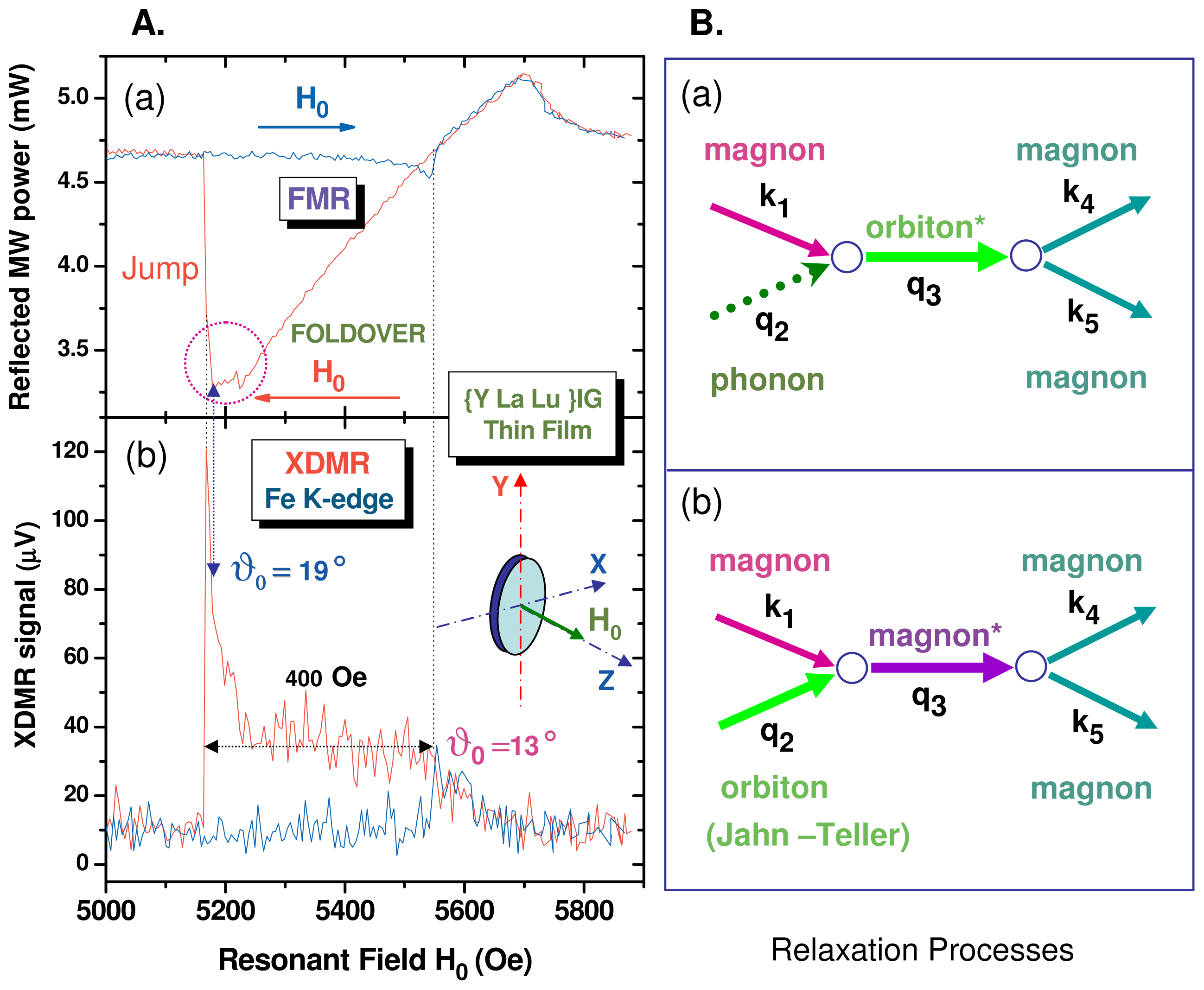
2.4.3. Mode Conversion in Relaxation Processes
2.5. Pseudo-Spin and Orbital Ordering Waves
is modulated by an operator
 which looks like the orbital quadrupole-quadrupole interaction (
 ) between sites i and j, i.e., the higher-order terms in the Van Vleck anisotropic exchange interaction. Note that
also appears in the theory of the Jahn–Teller effect. and that of the spin wave Hamiltonian for antiferromagnetic interactions. In order to solve the superexchange problem of Equation 25, Khaliullin [25] proposed to split
in three terms:
) between sites i and j, i.e., the higher-order terms in the Van Vleck anisotropic exchange interaction. Note that
also appears in the theory of the Jahn–Teller effect. and that of the spin wave Hamiltonian for antiferromagnetic interactions. In order to solve the superexchange problem of Equation 25, Khaliullin [25] proposed to split
in three terms:2.6. Spin Wave Instability Regime at High Pumping Power
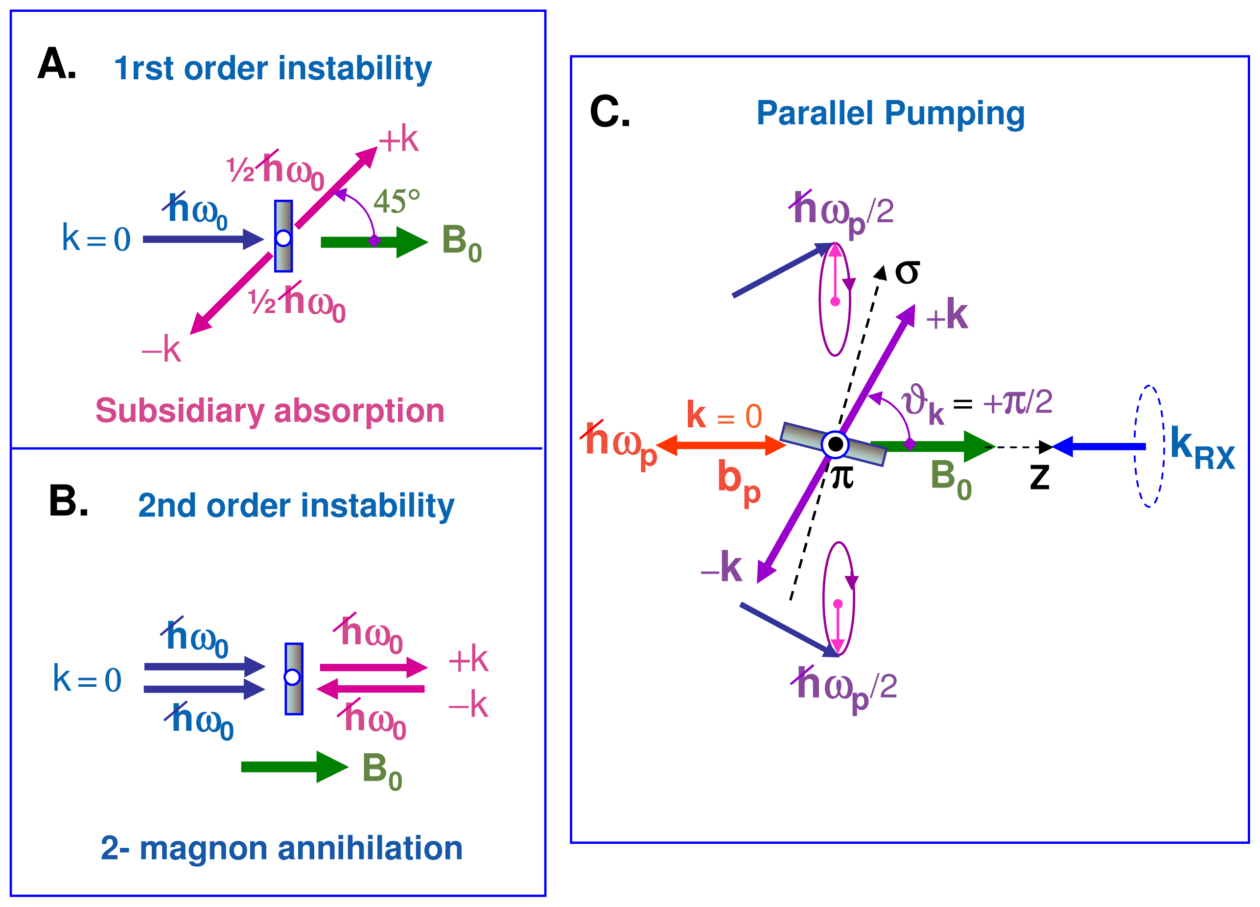
2.6.1. Transverse Pumping Geometry (bp ⊥ B0)
, one finally obtains for a perpendicularly magnetized thin film [20]:2.6.2. Parallel Pumping Geometry (bp || B0)
defined in Equation 20. This requires spin waves with elliptic precession of the magnetization vector, as expected for tangentially magnetized films. The onset of this parametric process is obtained for a threshold field given by:2.7. Instrumentation Constraints in XDMR Experiments
2.7.1. Soft-XMCD versus Hard-XMCD Probes
2.7.2. Combining Time and Frequency Domain Signals
3. XDMR in Ferrimagnetic Iron Garnets
3.1. Selected Samples
) and octahedral (
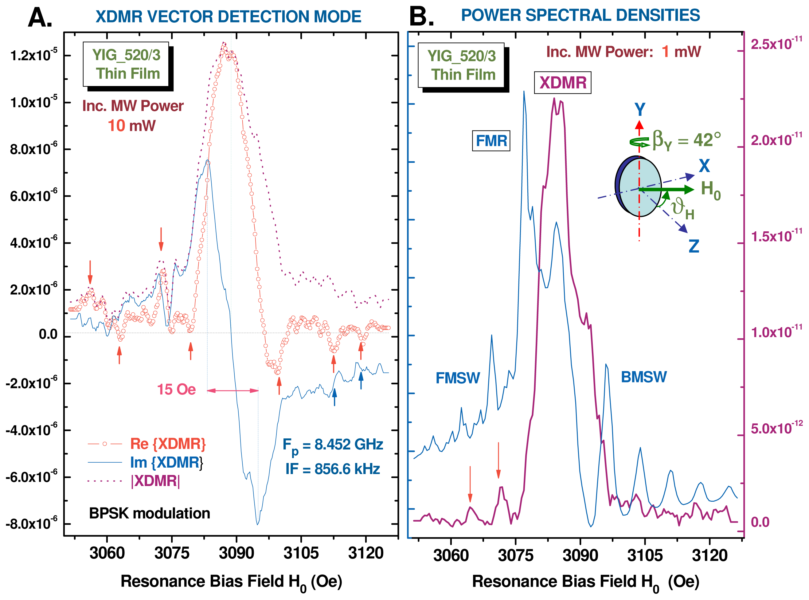
) iron sites. Below the magnetic ordering temperature (Tc ≃ 550 K), the two Fe sublattices get magnetized antiparallel one to each other, with an unbalanced magnetization (ca. 5 μB) in favor of the tetrahedral sites. The ferrimagnetic order is caused by a strong superexchange interaction between the two iron sublattices, the rather large Fe(16a)–O–Fe(24d) angles (126.6°) giving a clear indication that the wavefunctions of oxygen and iron have a substantial overlap. YIG is the generic term for a rich family of iron garnets in which yttrium can be substituted with rare earths in variable proportions.3.2. XDMR Spectra of a YIG Thin Film Recorded in Transverse Detection Geometry
3.3. Element Resolved XDMR of the Y-La-LuIG Film in Longitudinal Detection Geometry
site in the Y-La-LuIG film. Owing to the fact that the orbital magnetization components 〈ℓz〉 are heavily quenched at the rare earth sites [33], no significant relaxation anomaly can be detected at the La or Lu L-edges. This nicely illustrates the different nature of the relaxation mechanisms at different magnetic sites.3.4. Anomalous Saturation of the Fe K-Edge XDMR Spectra of GdIG
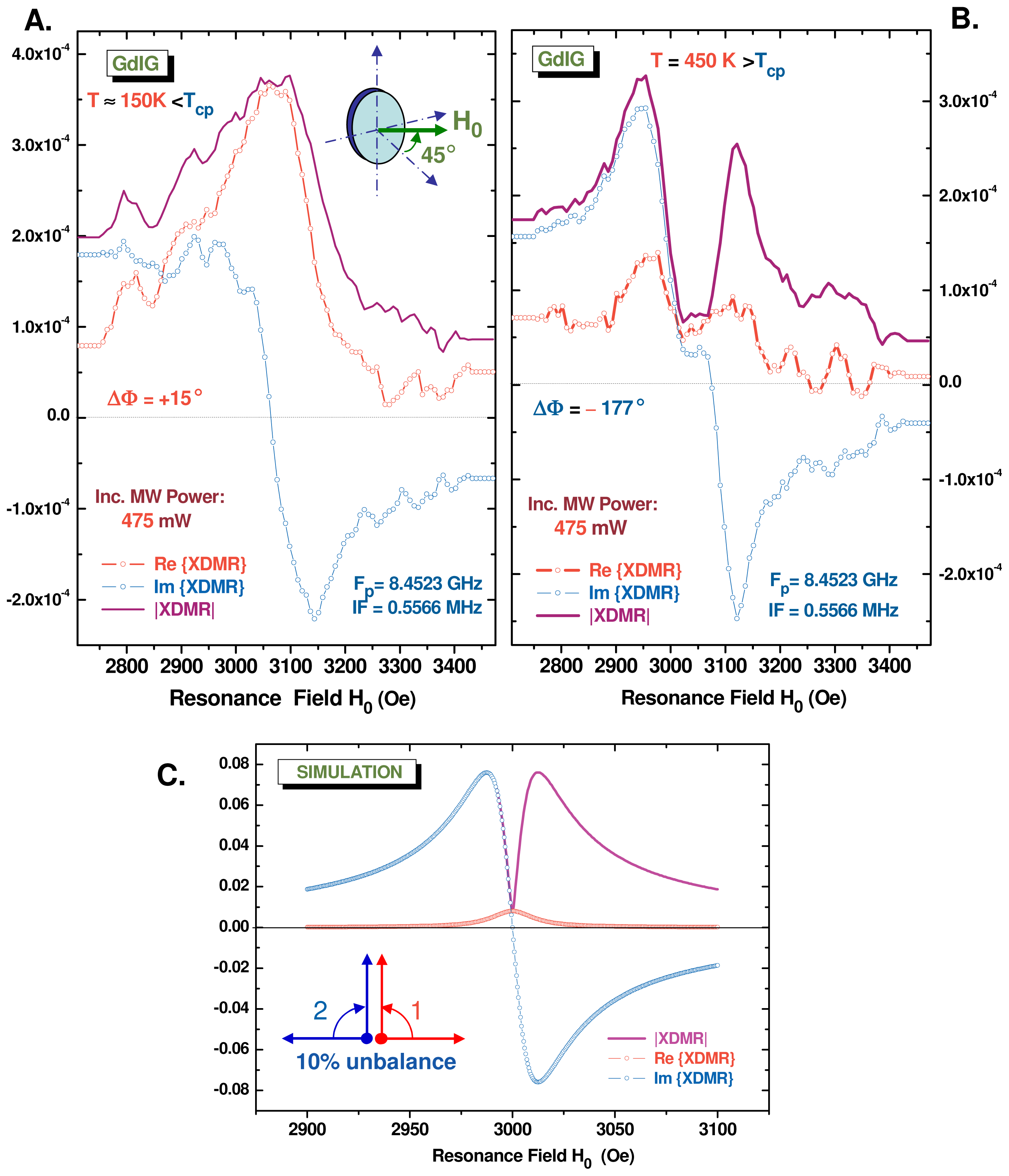
iron sites (24d). It is our interpretation that this anomaly is typical of a destructive interference between two resonant modes precessing in opposite senses as illustrated (for example) with Figure 6C. In other terms, the polarization of the precession is getting strongly elliptical. Complementary experiments revealed that this anomaly strongly depended on the pumping power and decreased on increasing the temperature. This looks like a possible signature—in the transverse detection geometry—of a 4-magnon scattering process in which the two scattered magnons with wavevectors +k and −k had strictly opposite helicities. We suspect the destructive interference to be particularly spectacular because the linewidth of the non uniform modes (±k) should be (again) much shorter than the linewidth of the degenerate uniform mode. which depends mostly on dipole-dipole interactions. It is not totally clear as yet why no similar anomaly did show up below the compensation temperature, i.e., in Figure 6A. It is hard to anticipate what exact role the Gd spins play in the intermediate temperature range above the ordering temperature TB and below Tcp. Note that 57Fe spin-echo NMR spectra recorded well below TB have established that the Gd spins were coupled to the Fe spins in the tetrahedral (24d) sites, the exchange integral Jdc amounting to only ≃ 12% of the exchange integral Jad describing the strong ferrimagnetic coupling of the iron sites [70,71]. Further work is in progress in order to compare the saturation properties of low temperature XDMR spectra recorded at the Fe K-edge and at the Gd L-edges.
3.5. Non-Linear Effects Associated With Elliptical Precession
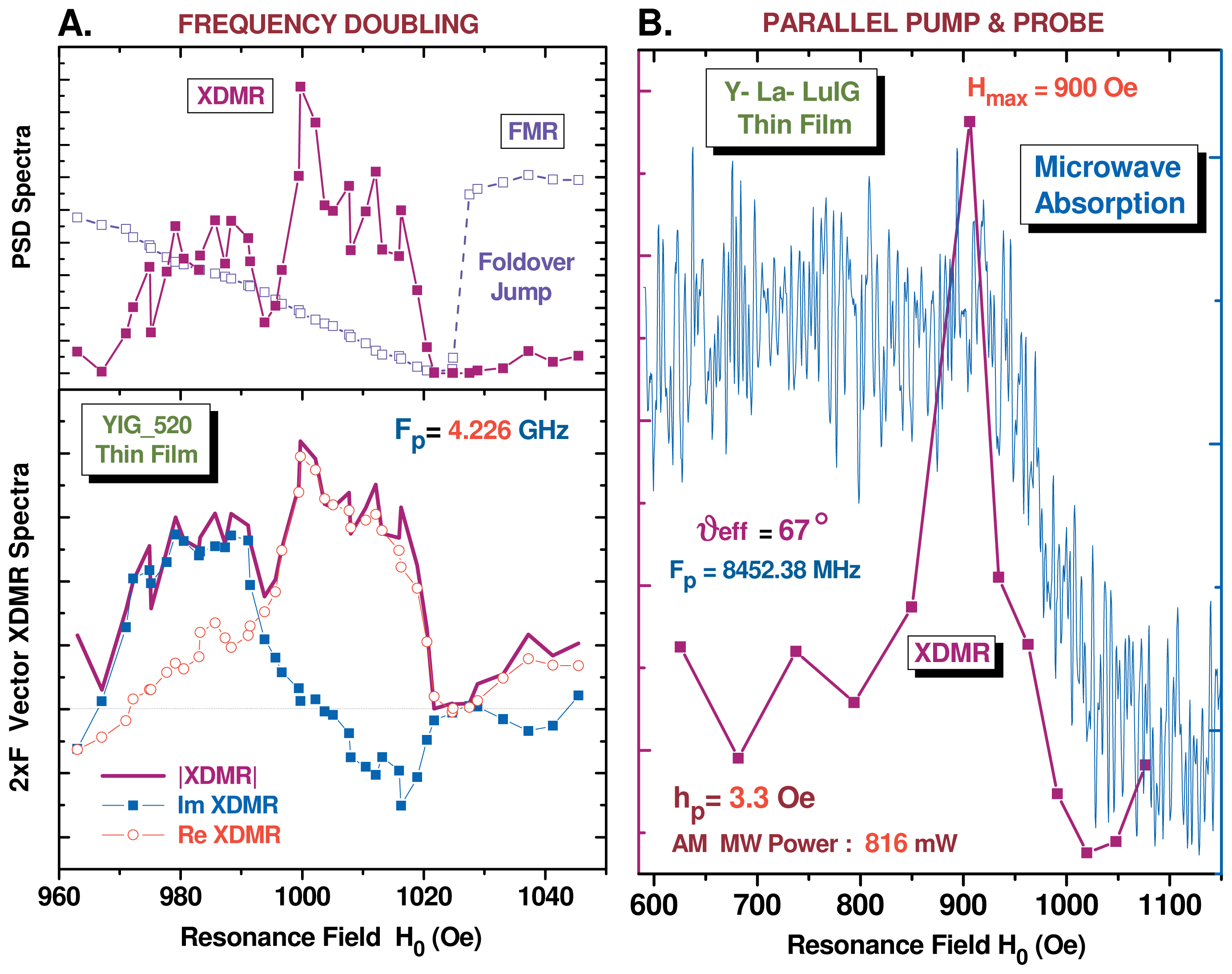
3.5.1. Second Harmonic XDMR Spectra in YIG Thin Films
3.5.2. XDMR under Parallel Pumping Excitation
4. New Challenges for XDMR
4.1. High-Field, X-Ray Detected Electron Paramagnetic Resonance
4.2. High-Field XDMR in the AFMR Regime
 TiO3, with
= Fe,Co) could also be good candidates for XDMR: they had rather low Néel temperatures [88,94] and significant orbital moments 〈Lz〉 at the sites of the Jahn–Teller cations [95]. With a much higher exchange field combined to a low anisotropy field [88,96], the case of Cr2O3 (TN = 308 K) looks less favorable even though we already produced definitive evidence of orbital magnetism in this crystal, at least in its magnetoelectric phase [97]. Although the spin-flop critical field of Cr2O3 is rather low (BC1 ≃ 5.9 T), it cannot be taken yet for granted that Δm⊥(±)will be large enough to yield a XDMR signal easily detectable at microwave pumping frequencies.
TiO3, with
= Fe,Co) could also be good candidates for XDMR: they had rather low Néel temperatures [88,94] and significant orbital moments 〈Lz〉 at the sites of the Jahn–Teller cations [95]. With a much higher exchange field combined to a low anisotropy field [88,96], the case of Cr2O3 (TN = 308 K) looks less favorable even though we already produced definitive evidence of orbital magnetism in this crystal, at least in its magnetoelectric phase [97]. Although the spin-flop critical field of Cr2O3 is rather low (BC1 ≃ 5.9 T), it cannot be taken yet for granted that Δm⊥(±)will be large enough to yield a XDMR signal easily detectable at microwave pumping frequencies.5. Conclusions
Acknowledgements
References
- Thole, B.T.; Carra, P.; Sette, F.; van der Laan, G. X-ray circular dichroism as a probe of orbital magnetization. Phys. Rev. Lett 1992, 68, 1943–1946. [Google Scholar]
- Carra, P.; Thole, B.T.; Altarelli, M.; Wang, X. X-ray circular dichroism and local magnetic fields. Phys. Rev. Lett 1993, 70, 694–697. [Google Scholar]
- Carra, P.; König, H.; Thole, B.T.; Altarelli, M. Magnetic X-ray X-ray dichroism. Physica B 1993, 192, 182–190. [Google Scholar]
- Goulon, J.; Rogalev, A.; Gauthier, Ch.; Goulon-Ginet, Ch.; Pasté, S.; Signorato, R.; Neumann, R.; Varga, L.; Malgrange, C. Instrumentation developments for X-ray linear and circular dichroism at the ESRF beamline ID12A. J. Synchrotron Radiat. 1998, 5, 232–238. [Google Scholar]
- Rogalev, A.; Goulon, J.; Goulon-Ginet, Ch.; Malgrange, C. Instrumentation Developments for Polarization Dependent X-Ray Spectroscopies at The ESRF Beamline ID12. In Magnetism and Synchrotron Radiation Approach; Beaurepaire, E., Scheurer, F., Krill, G., Kappler, J.-P., Eds.; Springer-Verlag: Berlin, Heidelberg, Germany, 2001; Volume 565, pp. 60–86. [Google Scholar]
- Goulon, J.; Rogalev, A.; Wilhelm, F.; Jaouen, N.; Goulon-Ginet, Ch.; Goujon, G.; Ben Youssef, J.; Indenbom, M.V. X-ray detected magnetic resonance at the Fe K-edge in YIG: Forced precession of orbital magnetization components. JETP Lett. 2005, 82, 791–796. [Google Scholar]
- Goulon, J.; Rogalev, A.; Wilhelm, F.; Jaouen, N.; Goulon-Ginet, Ch.; Brouder, Ch. X-ray detected ferromagnetic resonance in thin films. Eur. Phys. J. B 2006, 53, 169–184. [Google Scholar]
- Goulon, J.; Rogalev, A.; Wilhelm, F.; Goulon-Ginet, Ch.; Goujon, G. Element-selective X-ray detected magnetic resonance: A novel application of synchrotron radiation. J. Synchrotron Radiat. 2007, 14, 257–271. [Google Scholar]
- Goulon, J.; Rogalev, A.; Wilhelm, F.; Goujon, G. X-Ray Detected Magnetic Resonance. In Magnetism and Synchrotron Radiation; Beaurepaire, E., Bulou, H., Scheurer, F., Kappler, J.-P., Eds.; Springer Verlag: Berlin, Heidelberg, Germany, 2010; pp. 191–222. [Google Scholar]
- Goulon, J.; Rogalev, A.; Wilhelm, F.; Goujon, G.; Brouder, Ch.; Yaresko, A.; Ben Youssef, J.; Indenbom, M.V. X-ray detected magnetic resonance of YIG thin films in the non-linear regime of spin waves. J. Magn. Magn. Mater. 2010, 322, 2308–2329. [Google Scholar]
- Kittel, C. On the gyromagnetic ratio and spectroscopic splitting factor of ferromagnetic substances. Phys. Rev 1949, 76, 743–748. [Google Scholar]
- Blume, M.; Geschwind, G.; Yafet, A. Generalized kittel-van vleck relation between g and g′: Validity for negative g factors. Phys. Rev 1969, 181, 478–487. [Google Scholar]
- Van Vleck, J.H. Concerning the theory of ferromagnetic resonance absorption. Phys. Rev 1950, 78, 266–330. [Google Scholar]
- Van Kranendonk, J.; Van Vleck, J.H. Spin waves. Rev. Mod. Phys 1958, 30, 1–23. [Google Scholar]
- Kanamori, J. Anisotropy and Magnetostriction of Ferromagnetic and Antiferromagnetic Materials. In Magnetism; Suhl, H., Rado, G.T., Eds.; Academic Press Inc: New York NY, USA, 1963; Volume 1, Chapter 4; pp. 127–203. [Google Scholar]
- Stevens, K.W.H. Spin Hamiltonians. In Magnetism; Suhl, H., Rado, G.T., Eds.; Academic Press Inc: New York NY, USA, 1963; Volume 1, Chapter 1; pp. 1–23. [Google Scholar]
- Abragam, A.; Bleaney, B. Electron Paramagnetic Resonance of Transition Ions; Oxford University Press: Oxford, UK, 1970. [Google Scholar]
- Pryce, M.H.L. Sign of g in magnetic resonance, and the sign of the quadrupole moment of 237Np. Phys. Rev. Lett 1959, 3, 375–376. [Google Scholar]
- Elliott, R.J.; Thorpe, M.F. Orbital effects on exchange interactions. J. Appl. Phys 1968, 39, 802–807. [Google Scholar]
- Gurevich, A.G.; Melkov, G.A. Magnetization Oscillations and Waves; CRC Press Inc: Boca Raton, FL USA, 1996. [Google Scholar]
- Mozhegorov, A.A.; Larin, A.V.; Nikiforov, A.E.; Gontchar, L.E.; Efremov, A.V. Theory of magnetic resonance as an orbital state probe. Phys. Rev. B 2009, 79, 054418:1–054418:8. [Google Scholar]
- Anderson, P.W. Exchange in Insulators: Superexchange, Direct Exchange and Double Exchange. In Magnetism; Suhl, H., Rado, G.T., Eds.; Academic Press Inc: New York NY, USA, 1963; Volume 1, Chapter 2; pp. 25–83. [Google Scholar]
- Kugel’, K.I.; Khomskii, D.I. The Jahn-Teller effect in magnetism: Transition metal compounds. Sov. Phys. Uspekhi 1982, 25, 231–256. [Google Scholar]
- Cyrot, M.; Lyon-Caen, C. Orbital superlattice in the degenerate Hubbard model. J. Phys 1975, 36, 253–266. [Google Scholar]
- Khaliullin, G. Quantum effects in Orbitally Degenerate Systems. In Physics of Transition Metal Oxides; Cardona, M., Fulde, P., von Klitzing, K., Merlin, R., Queisser, H.-J., Störmer, H., Eds.; Springer Verlag: Berlin, Heidelberg, Germany, 2004; Volume 144, Chapter 7; pp. 261–308. [Google Scholar]
- Rogalev, A.; Wilhelm, F.; Jaouen, N.; Goulon, J.; Kappler, J.-P. X-ray Magnetic Circular Dichroism: Historical Perspective and Recent Highlights. In Magnetism: A Synchrotron Radiation Approach; Beaurepaire, E., Bulou, H., Scheurer, F., Kappler, J.-P., Eds.; Springer-Verlag: Berlin, Heidelberg, Germany, 2006; pp. 71–94. [Google Scholar]
- Strange, P. Magnetic absorption and sumrules in itinerant magnets. J. Phys. Condens. Matter 1994, 6, L491–L495. [Google Scholar]
- Guo, G.Y. What does the K-edge X-ray magnetic circular dichroism spectrum tell us? J. Phys. Condens. Matter 1996, 8, L747–L752. [Google Scholar]
- Ebert, H.; Popescu, V.; Ahlers, D. Fully relativistic theory for magnetic EXAFS: Formalism and applications. Phys. Rev. B 1999, 60, 7156–7165. [Google Scholar]
- Stöhr, J.; König, H. Determination of spin- and orbital-moment anisotropies in transition metals by angle-dependent X-ray magnetic circular dichroism. Phys. Rev. Lett 1995, 75, 3748–3751. [Google Scholar]
- Van der Laan, G. Microscopic origin of magnetocrystalline anisotropy in transition metal thin films. J. Phys. Condens. Matter 1998, 10, 3239–3253. [Google Scholar]
- Yaresko, A.N.; Perlov, A.; Antonov, V.; Harmon, B. Band-Structure Theory of Dichroism. In Magnetism: A Synchrotron Radiation Approach; Beaurepaire, E., Bulou, H., Scheurer, F., Kappler, J.-P., Eds.; Springer-Verlag: Berlin, Heidelberg, Germany, 2006; Volume 697, pp. 121–141. [Google Scholar]
- Rogalev, A.; Goulon, J.; Wilhelm, F.; Brouder, Ch.; Yaresko, A.; Ben Youssef, J.; Indenbom, M.V. Element selective X-ray magnetic circular and linear dichroisms in ferrimagnetic yttrium iron garnet films. J. Magn. Magn. Mater. 2009, 321, 3945–3962. [Google Scholar]
- Stancil, D.D. Theory of Magnetostatic Waves; Springer-Verlag: Berlin, Heidelberg, Germany, 1993; pp. 1–173. [Google Scholar]
- Nazarov, A.V.; Patton, C.E.; Cox, R.G.; Chen, L.; Kabos, P. General spin wave instability theory for anisotropic ferromagnetic insulators at high microwave power levels. J. Magn. Magn. Mater 2002, 248, 164–180. [Google Scholar]
- Jander, A.; Moreland, J.; Kabos, P. Angular momentum and energy transferred through ferromagnetic resonance. Appl. Phys. Lett 2001, 78, 2348–2350. [Google Scholar]
- Holstein, T.; Primakoff, H. Field dependence of the intrinsic domain magnetization of a ferromagnet. Phys. Rev 1940, 58, 1098–1113. [Google Scholar]
- Sparks, M. Ferromagnetic Relaxation Theory; McGraw-Hill: New York NY, USA, 1964; pp. 1–227. [Google Scholar]
- Keffer, F. Spin Waves. In Handbuch der Physik; Springer-Verlag: Berlin, Heidelberg, Germany, 1966; Volume XVIII, pp. 1–268. [Google Scholar]
- Akhiezer, A.I.; Baryakthar, V.G.; Peletminskii, S.V. Doniach, S., Ed.; North Holland Publ. Co.: Amsterdam, The Netherlands, 1968; Volume 1, pp. 1–369.
- Cottam, M.G.; Slavin, A.N. Fundamentals of Linear and Nonlinear Spin Wave Processes in Bulk and Finite Magnetic Samples. In Linear and Nonlinear Spin Waves in Magnetic Films and Superlattices; Cottam, M.G., Ed.; World Scientific Publ. Co. Pte. Ltd.: Singapore, 1994; Volume Chapter 1, pp. 1–88. [Google Scholar]
- Timm, C. Theory of Magnetism; Lecture at the International Max Planck Research School for Dynamical Processes in Atoms, Molecules and Solids; April 2011; pp. 1–93. [Google Scholar]
- Schlömann, E. Longitudinal susceptibility of ferromagnets in strong rf fields. J. Appl. Phys 1962, 33, 527–537. [Google Scholar]
- Suhl, H. The theory of ferromagnetic resonance at high signal power. J. Phys. Chem. Solids 1957, 1, 209–227. [Google Scholar]
- Suhl, H. Note on the saturation of the main resonance in ferromagnetics. J. Appl. Phys 1959, 30, 1961–1964. [Google Scholar]
- Suhl, H. “Foldover” effects caused by spin wave interactions in ferromagnetic resonance. J. Appl. Phys 1960, 31, 935–936. [Google Scholar]
- Suhl, H. Restoration of stability in ferromagnetic resonance. Phys.Rev. Lett 1961, 6, 174–176. [Google Scholar]
- Damon, R.W. Ferromagnetic Resonance at High Power. In Magnetism; Suhl, H., Rado, G.T., Eds.; Academic Press Inc: New York, NY, USA, 1963; Volume 1, Chapter 11; pp. 551–620. [Google Scholar]
- Haas, C.W.; Callen, H.B. Ferromagnetic Relaxation and Resonance Line Widths. In Magnetism; Suhl, H., Rado, G.T., Eds.; Academic Press Inc: New York, NY, USA, 1963; Volume 1, Chapter 10; pp. 449–549. [Google Scholar]
- Bailey, W.E.; Cheng, L.; Keavney, D.J.; Kao, C.-C.; Vescovo, E.; Arena, D.A. Precessional dynamics of elemental moments in a ferromagnetic alloy. Phys. Rev. B 2004, 70, 172403:1–172403:4. [Google Scholar]
- Arena, D.A.; Vescovo, E.; Kao, C.-C.; Guan, Y.; Bailey, W.E. Weakly coupled motion of individual layers in ferromagnetic resonance. Phys. Rev. B 2006, 74, 064409:1–064409:7. [Google Scholar]
- Guan, Y.; Bailey, W.E.; Kao, C.-C.; Vescovo, E.; Arena, D.A. Comparison of time-resolved X-ray magnetic circular dichroism measurements in reflection and transmission for layer specific precessional dynamics measurements. J. Appl. Phys 2006, 99, 08J305:1–08J305:3. [Google Scholar]
- Arena, D.A.; Vescovo, E.; Kao, C.-C.; Guan, Y.; Bailey, W.E. Combined time-resolved X-ray magnetic circular dichroism and ferromagnetic resonance studies of magnetic alloys and multilayers. J. Appl. Phys 2007, 101, 09C109:1–09C109:6. [Google Scholar]
- Guan, Y.; Bailey, W.E.; Vescovo, E.; Kao, C.-C.; Arena, D.A. Phase and Amplitude of element-specific moment precession in Ni81Fe19. J. Mag. Magn. Mater 2007, 312, 374–378. [Google Scholar]
- Arena, D.A.; Ding, Y.; Vescovo, E.; Zohar, S.; Guan, Y.; Bailey, W.E. A compact apparatus for studies of element and phase-resolved ferromagnetic resonance. Rev. Sci. Instrum 2009, 80, 083903:1–083903:7. [Google Scholar]
- Boero, G.; Rusponi, S.; Bencock, P.; Popovic, R.S.; Brune, H.; Gambardella, P. X-ray ferromagnetic resonance spectroscopy. Appl. Phys. Lett 2005, 87, 152503:1–152503:3. [Google Scholar]
- Boero, G.; Mouaziz, S.; Rusponi, S.; Bencok, P.; Nolting, S.; Stepanow, S.; Gambardella, P. Element-resolved X-ray ferrimagnetic and ferromagnetic resonance spectroscopy. New J. Phys 2008, 10, 013011:1–013011:16. [Google Scholar]
- Boero, G.; Rusponi, S.; Bencok, P.; Meckenstock, R.; Thiele, J.-U.; Nolting, F.; Gambardella, P. Double-resonant X-ray and microwave absorption: Atomic spectroscopy and precessional orbital and spin dynamics. Phys. Rev. B 2009, 79, 224425:1–224425:8. [Google Scholar]
- Boero, G.; Rusponi, S.; Kavich, J.; Lodi Rizzini, A.; Piamonteze, C.; Nolting, F.; Tieg, C.; Thiele, J.-U.; Gambardella, P. Longitudinal detection of ferromagnetic resonance using X-ray transmission measurements. Rev. Sci. Instrum 2009, 80, 123902:1–123902:11. [Google Scholar]
- Marcham, M.K.; Keatley, P.S.; Neudert, A.; Hicken, R.J.; Cavill, S.A.; Shelford, L.R.; van der Laan, G.; Telling, N.D.; Childress, J.R.; Katine, J.A.; Shafer, P.; Arenholz, E. Phase resolved X-ray ferromagnetic resonance measurements in fluorescence yield. J. Appl. Phys 2011, 109, 07D353:1–07D353:3. [Google Scholar]
- Gilleo, M.A. Ferromagnetic Insulators: Garnets. In Ferromagnetic Materials; Wohlfarth, E.P., Ed.; North-Holland Publ. Co.: Amsterdam, The Netherlands, 1980; Volume 2, pp. 1–53. [Google Scholar]
- Phillips, T.G.; Rosenberg, H.M. Spin waves in ferromagnets. Rep. Prog. Phys 1966, 29, 285–332. [Google Scholar]
- Kasuya, T.; LeCraw, R.C. Relaxation mechanism in Ferromagnetic Resonance. Phys. Rev. Lett. 1961, 6, 223–225. [Google Scholar]
- Schlömann, E. Fine structure in the decline of the ferromagnetic resonance abasorption with increasing power level. Phys. Rev 1959, 116, 828–837. [Google Scholar]
- Hansen, P. Magnetic Anisotropy and Magnetostriction in Garnets. In Physics of Magnetic Garnets; Paoletti, A., Ed.; North-Holland: Amsterdam, The Netherlands; New York, NY, USA, 1978; Volume LXX, pp. 56–133. [Google Scholar]
- Van Vleck, J.H.; Orbach, R. Ferrimagnetic resonance of dilute rare-earth doped iron garnets. Phys. Rev. Lett 1963, 11, 65–67. [Google Scholar]
- Van Vleck, J.H. Ferrimagnetic resonance of rare-earth doped iron garnets. J. Appl. Phys 1964, 35, 882–888. [Google Scholar]
- Belov, K.P. Ferrimagnets with a “weak” magnetic sublattice. Physics-Uspekhi 1996, 39, 623–634. [Google Scholar]
- Geschwind, S.; Walker, L.R. Exchange resonance in gadolinium iron garnet near the magnetic compensation temperature. J. Appl. Phys 1959, 30, 163S–170S. [Google Scholar]
- Litster, J.D.; Benedek, G.B. NMR study of iron sublattice magnetization in YIG and GdIG. J. Appl. Phys 1966, 37, 1320–1322. [Google Scholar]
- Myers, S.M.; Gonano, R.; Meyer, H. Sublattice magnetization of several rare-earth iron garnets. Phys. Rev 1968, 170, 513–519. [Google Scholar]
- Schlömann, E. Fine structure in the decline of the ferromagnetic resonance absorption with increasing power level. Phys. Rev 1959, 116, 828–837. [Google Scholar]
- Goulon, J.; Rogalev, A.; Goujon, G.; Wilhelm, F.; Brouder, Ch. X-ray detected magnetic resonance of YIG thin films under tangential and oblique parallel pumping. J. Magn. Magn. Mater 2012. to be submitted.. [Google Scholar]
- Goulon, J.; Rogalev, A.; Wilhelm, F.; Goujon, G.; Idehara, T. Sub-THz gyrotron optimized for X-ray detected electron magnetic resonance. J. Plasma Fusion Res 2008, 84, 909–911. [Google Scholar]
- Rogalev, A.; Goulon, J.; Goujon, G.; Wilhelm, F.; Ogawa, I.; Idehara, T. X-ray Detected Magnetic Resonance at Sub-THz frequencies using a high power gyrotron source. J. Infrared Milli. Terahz. Waves 2012, in press. [Google Scholar]
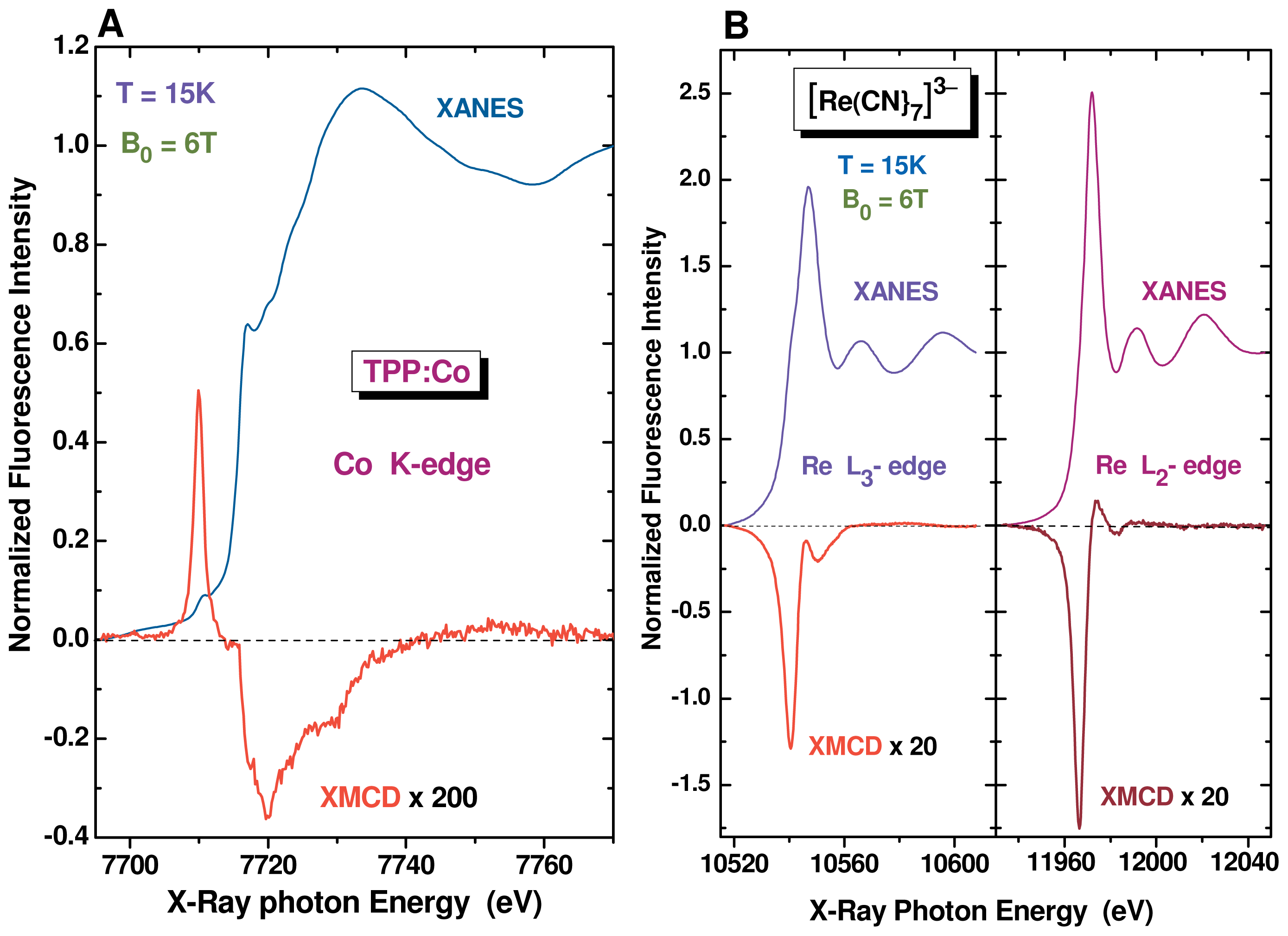
- Benett, M.V.; Long, J.R. New cyanometalate building units: Synthesis and characterization of [Re(CN)7]3− and [Re(CN)8]3−. J. Am. Chem. Soc 2003, 125, 2394–2395. [Google Scholar]
- Freedman, D.E.; Jenkins, D.M.; Iavarone, A.T.; Long, J.R. A redox-switchable single-molecule magnet incorporating [Re(CN)7]3−. J. Am. Chem. Soc 2008, 130, 2884–2885. [Google Scholar]
- Walker, F.A.V. Proton NMR, EPR Spectroscopy of Paramagnetic Metalloporphyrins. In The Porphyrin Handbook; Kadish, K.M., Smith, K.M., Guilard, R., Eds.; Academic Press: New York, NY, USA, 2000; Volume 6, Chapter 36; pp. 82–175. [Google Scholar]
- Goulon, J.; Goulon-Ginet, Ch.; Gotte, V. X-ray Absorption Spectroscopy Applied to Porphyrin Chemistry. In The Porphyrin Handbook; Kadish, K.M., Smith, K.M., Guilard, R., Eds.; Academic Press: New York, NY, USA, 2000; Volume 7, Chapter 49; pp. 79–166. [Google Scholar]
- Bowman, M.K.; Fourier, Transform; Electron, Spin. Resonance. In Modern Pulsed and Continuous-Wave Electron Spin Resonance; Kevan, L., Bowman, M.K., Eds.; John Wiley & Sons Inc: New York, NY, USA, 1990; pp. 1–42. [Google Scholar]
- Smith, G.M.; Riedi, P.C. Progress in High Field EPR. In Electron Paramagnetic Resonance; RSC Publishing: Cambridge, UK, 2000; Volume 17, Chapter 6; pp. 164–204. [Google Scholar]
- Morley, G.W.; Brunel, L.-C.; van Tol, J. A multifrequency high field pulsed electron paramagnetic resonance/electron-nuclear double resonance spectrometer. Rev. Sci. Instrum 2008, 79, 064703:1–064703:5. [Google Scholar]
- Savitsky, A.; Moebius, K. High field EPR. Photosynth. Res 2009, 102, 311–333. [Google Scholar]
- Anderson, P.W.; Weiss, P.R. Exchange narrowing in paramagnetic resonance. Rev. Mod. Phys 1953, 25, 269–276. [Google Scholar]
- Cage, B.; Cevc, P.; Blinc, R.; Brunel, L.-C.; Dalal, N.S. 1–370 GHz EPR linewidths for K3CrO8: A comprehensive test for the anderson-weiss model. J. Magn. Reson 1998, 135, 178–184. [Google Scholar]
- Krzystek, J.; Ozarowski, A.; Telser, J. Multi-frequency, high-field EPR as a powerful tool to accurately determine zero-field splitting in high-spin transition metals coordination complexes. Coord. Chem. Rev 2006, 250, 2308–2324. [Google Scholar]
- Tagirov, M.S.; Tayurskii, D.A. Insulating Van Vleck paramagnets at high magnetic fields (Review). Low Temp. Phys 2002, 28, 147–164. [Google Scholar]
- Foner, S. Antiferromagnetic and Ferrimagnetic Resonance. In Magnetism; Suhl, H., Rado, G.T., Eds.; Academic Press Inc: New York, NY, USA, 1963; Volume 1, Chapter 9; pp. 383–447. [Google Scholar]
- Kotthaus, J.P.; Jaccarino, V. Antiferromagnetic-resonance linewidth in MnF2. Phys. Rev. Lett 1972, 28, 1649–1652. [Google Scholar]
- Lui, M.; King, A.R.; Kotthaus, J.P.; Hansma, P.K.; Jaccarino, V. Observation of antiferromagnetic resonance in epitaxial films of MnF2. Phys. Rev. B 1986, 33, 7720–7723. [Google Scholar]
- Pavarini, E.; Koch, E.; Lichtenstein, A.I. Mechanism for orbital ordering in KCuF3. Phys. Rev. Lett 2008, 101, 2666405:1–2666405:4. [Google Scholar]
- Kato, N.; Yamada, I. Multi-sublattice magnetic structure of KCuF3 caused by the antisymmetric exchange interaction: Antiferromagnetic resonance measurements. J. Phys. Soc. Jpn 1994, 63, 289–297. [Google Scholar]
- Moriya, T. Weak Ferromagnetism. In Magnetism; Suhl, H., Rado, G.T., Eds.; Academic Press Inc: New York, NY, USA, 1963; Volume 1, Chapter 3; pp. 85–125. [Google Scholar]
- Stickler, J.J.; Kern, S.; Wold, A.; Heller, G.S. Magnetic resonance and susceptibility of several ilmenite powders. Phys. Rev 1967, 164, 765–767. [Google Scholar]
- McDonald, P.F.; Parasiris, A.; Pandey, R.K.; Gries, B.L.; Kirk, W.P. Paramagnetic resonance and susceptibility of ilmenite FeTiO3 crystal. J. Appl. Phys 1991, 69, 1104–1106. [Google Scholar]
- Foner, S. High-field antiferromagnetic resonance in Cr2O3. Phys. Rev 1963, 130, 183–197. [Google Scholar]
- Goulon, J.; Rogalev, A.; Wilhelm, F.; Goulon-Ginet, C.; Carra, P.; Marri, I.; Brouder, C. X-ray optical activity: Applications of sum rules. J. Exp. Theor. Phys 2003, 97, 402–431. [Google Scholar]
and S6 at the Fe (24d) and Fe (16a) crystal sites in YIG: opposite signs were expected due to the antiferromagnetic coupling of the Fe cations in (24d) and (16a) sites; (B) Simulated XMCD spectra in the energy range of the Fe K-edge pre-peak. Note that the XMCD signal due to electric dipole transitions (E1) is much stronger at the tetrahedral (
) than at the octahedral (
) coordination sites. The contributions of electric quadrupole transitions (E2) are one order of magnitude weaker.


© 2011 by the authors; licensee MDPI, Basel, Switzerland. This article is an open-access article distributed under the terms and conditions of the Creative Commons Attribution license (http://creativecommons.org/licenses/by/3.0/).
Share and Cite
Goulon, J.; Rogalev, A.; Goujon, G.; Wilhelm, F.; Youssef, J.B.; Gros, C.; Barbe, J.-M.; Guilard, R. X-Ray Detected Magnetic Resonance: A Unique Probe of the Precession Dynamics of Orbital Magnetization Components. Int. J. Mol. Sci. 2011, 12, 8797-8835. https://doi.org/10.3390/ijms12128797
Goulon J, Rogalev A, Goujon G, Wilhelm F, Youssef JB, Gros C, Barbe J-M, Guilard R. X-Ray Detected Magnetic Resonance: A Unique Probe of the Precession Dynamics of Orbital Magnetization Components. International Journal of Molecular Sciences. 2011; 12(12):8797-8835. https://doi.org/10.3390/ijms12128797
Chicago/Turabian StyleGoulon, José, Andrei Rogalev, Gérard Goujon, Fabrice Wilhelm, Jamal Ben Youssef, Claude Gros, Jean-Michel Barbe, and Roger Guilard. 2011. "X-Ray Detected Magnetic Resonance: A Unique Probe of the Precession Dynamics of Orbital Magnetization Components" International Journal of Molecular Sciences 12, no. 12: 8797-8835. https://doi.org/10.3390/ijms12128797