Abstract
When suspensions involving rigid rods become too concentrated, standard dilute theories fail to describe their behavior. Rich microstructures involving complex clusters are observed, and no model allows describing its kinematics and rheological effects. In previous works the authors propose a first attempt to describe such clusters from a micromechanical model, but neither its validity nor the rheological effects were addressed. Later, authors applied this model for fitting the rheological measurements in concentrated suspensions of carbon nanotubes (CNTs) by assuming a rheo-thinning behavior at the constitutive law level. However, three major issues were never addressed until now: (i) the validation of the micromechanical model by direct numerical simulation; (ii) the establishment of a general enough multi-scale kinetic theory description, taking into account interaction, diffusion and elastic effects; and (iii) proposing a numerical technique able to solve the kinetic theory description. This paper focuses on these three major issues, proving the validity of the micromechanical model, establishing a multi-scale kinetic theory description and, then, solving it by using an advanced and efficient separated representation of the cluster distribution function. These three aspects, never until now addressed in the past, constitute the main originality and the major contribution of the present paper.
1. Introduction
Short fibers, nanofibers or carbon nanotubes—CNT—suspensions present different morphologies, depending on their concentrations. When the concentration is dilute enough, one can describe the microstructure by tracking a population of rods that move with the suspending fluid and orient depending on the velocity gradient according to the Jeffrey’s equation [1] that relates the orientation evolution with the flow velocity field. In that case, the motion and orientation of each fiber is assumed decoupled from the others. The representative population can involve too many fibers, and in that case, the computational efforts to track the population is unaffordable. Thus, the simple and well-defined physics must be sacrificed in order to derive coarser descriptions.
Kinetic theory approaches [2,3,4] describe such systems at the mesoscopic scale. Their main advantage is their capability to address macroscopic systems, while keeping the fine physics through a number of conformational coordinates introduced for describing the microstructure and its time evolution. At this mesoscopic scale, the microstructure is defined from a distribution function that depends on the physical space, the time and a number of conformational coordinates—the rods orientation in the case of slender body suspensions. The moments of this distribution constitute a coarser description, in general, used in macroscopic modeling [5].
At the macroscopic scale, the equations governing the time evolution of these moments usually involve closure approximations, whose impact in the results is unpredictable [6,7,8]. Other times, macroscopic equations are carefully postulated in order to guarantee the model objectivity and its thermodynamical admissibility.
In the case of dilute suspensions of short fibers, the three scales have been extensively considered to model the associated systems without major difficulties. However, as soon as the concentration increases, the difficulties appear. In the semi-dilute and semi-concentrated regimes, fiber-fiber interactions occur, but in general, they can be accurately modeled by introducing a sort of randomizing diffusion term [9]. There is a wide literature concerning dilute and semi-dilute suspensions, addressing modeling [10,11,12,13,14], flows [15,16,17,18] and rheology [19,20]. These models describe quite well the experimental observations. When the concentration increases, rods interactions cannot be neglected anymore and appropriate models addressing these intense interactions must be considered, as, for example, the one proposed in [21]. Recent experiments suggest that short fibers in concentrated suspensions align more slowly as a function of strain than models based on Jeffery’s equation predict [22]. For addressing this issue, Wang et al. [22] proposed the use of a strain reduction factor; however, this solution violates objectivity. Later, the same authors proposed an objective model by decoupling the time evolution of both the eigenvalues and the eigenvectors of the second order orientation tensor [23]. In [24], an anisotropic rotary diffusion is proposed for accounting for the fiber-fiber interactions, and the model parameters were selected by matching the experimental steady-state orientation in simple shear flow and by requiring stable steady states and physically realizable solutions.
The worst scenario concerns concentrated suspensions involving entangled clusters exhibiting aggregation/disaggregation mechanisms. A first approach in that sense was proposed in [25]. The first natural question is how to describe such systems? At the macroscopic scale, one could try to fit some power-law constitutive equation; however, this description does not allow one to describe the microstructure. At the microscopic scale, direct numerical simulations describing complex fiber-fiber interactions can be carried out in small enough representative volumes [26,27]. A natural candidate to be a reasonable compromise between (fine) micro and (fast) macro descriptions consists of considering, again, a kinetic theory description.
The main issue of such an approach lies in the fact that it must include two scales, the one involving the aggregates and the one related to the rods composing the aggregates. What are the appropriate conformational coordinates? How does one determine the time evolution of these conformational coordinates? How does one represent, simultaneously, both scales, the one related to the aggregates and the other related to the fibers? How does one derive the interaction mechanisms?... These questions will be addressed in this work.
In [28], the authors propose a first attempt to describe such clusters from a micromechanical model, but neither its validity nor the rheological effects were addressed. Later, in [29], the authors applied this model for fitting the rheological measurements in concentrated suspensions of carbon nanotubes (CNTs) by assuming a rheo-thinning behavior at the constitutive law level. However, three major issues were never addressed until now: (i) the validation of the micromechanical model by direct numerical simulation; (ii) the establishment of a general enough multi-scale kinetic theory description, taking into account interaction, diffusion and elastic effects; and (iii) propose a numerical technique able to solve the kinetic theory description. This paper focuses on these three major issues, proving the validity of the micromechanical model, establishing a multi-scale kinetic theory description and, then, solving it by using an advanced and efficient separated representation of the cluster distribution function. These three aspects, never until now addressed in the past, constitute the main originality and the major contribution of the present paper.
In this paper, we first propose two micro-mechanical models for describing the kinematics of rigid and deformable aggregates in Section 2 and Section 3, respectively. The double scale kinetic theory model will be, then, addressed in Section 4. Section 5 considers different interaction mechanics in order to derive an extended kinetic theory model. The issues related to its numerical solution will be deeply analyzed in Section 6. Section 7 presents some verification and validation tests of the proposed micro-mechanical models, and finally, first numerical results are given in Section 8.
2. Micro-Mechanical Description of the Kinematics of Rigid Clusters
As just discussed, when the rod concentration is high enough, rod interactions cannot be neglected anymore, and appropriate models addressing these intense interactions must be addressed. In the extreme case, a sort of cluster composed of entangled rods is observed [25,30]. When the suspension flows, those clusters seem animated by almost rigid motions.
Clusters can be viewed as entangled aggregates of rods, with these rods consisting of a rigid segment joining the two beads located at the segment ends, where it is assumed that forces apply. Microscopic simulations become unaffordable, due to the computational resources needed to address scenarios of real interest. On the other hand, macroscopic modeling is without any doubt too phenomenological for describing the main flow and microstructure features. Kinetic theory approaches could be an appealing compromise between accuracy and computational efficiency.
In what follows, we consider the cluster idealization depicted in Figure 1 in the case of a hypothetical 2D aggregate that does not involve size effects, but at least involves the orientation distribution. Obviously, this representation is a crude simplification, but it constitutes the simplest model and could be later enriched, without major difficulties, to include more complex and richer configurations.
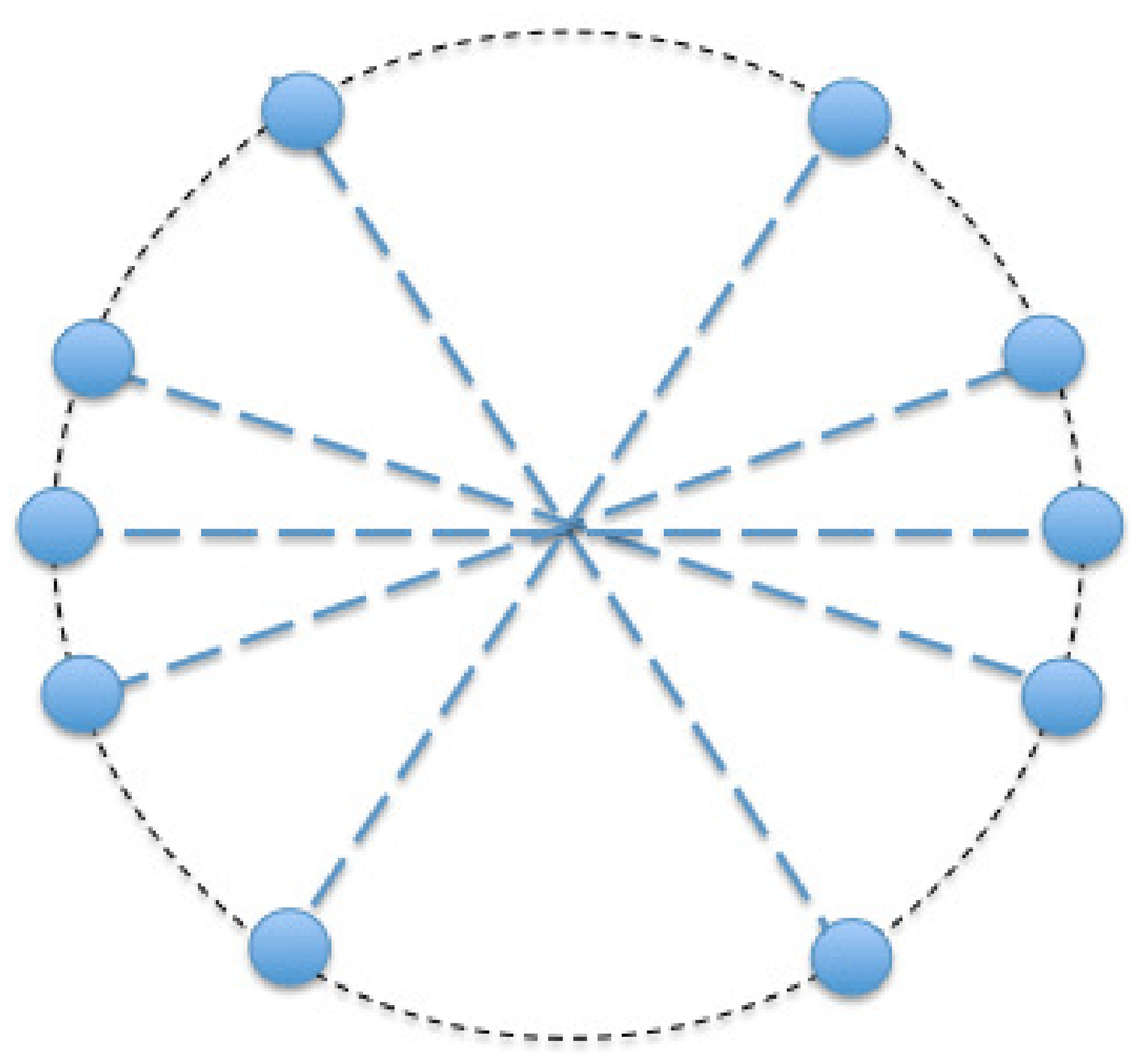
Figure 1.
Star representation of a cluster composed of rigid rods.
First, we consider a 2D rigid cluster consisting of N rods of length, , oriented in the directions, , , as sketched in Figure 2. Brownian effects can be neglected, and then, only flow induced hydrodynamic forces must be considered (the rod-rod hydrodynamic interactions are not considered in this work). Forces, , apply on each bead located at position, (Figure 2), and are proportional to the difference of velocity between the one flow unperturbed by the presence of the cluster at the bead location and the other one, the bead itself:
where ξ is the friction coefficient and the flow velocity field unperturbed by the cluster presence. We can notice that forces are, by construction, self-equilibrated.
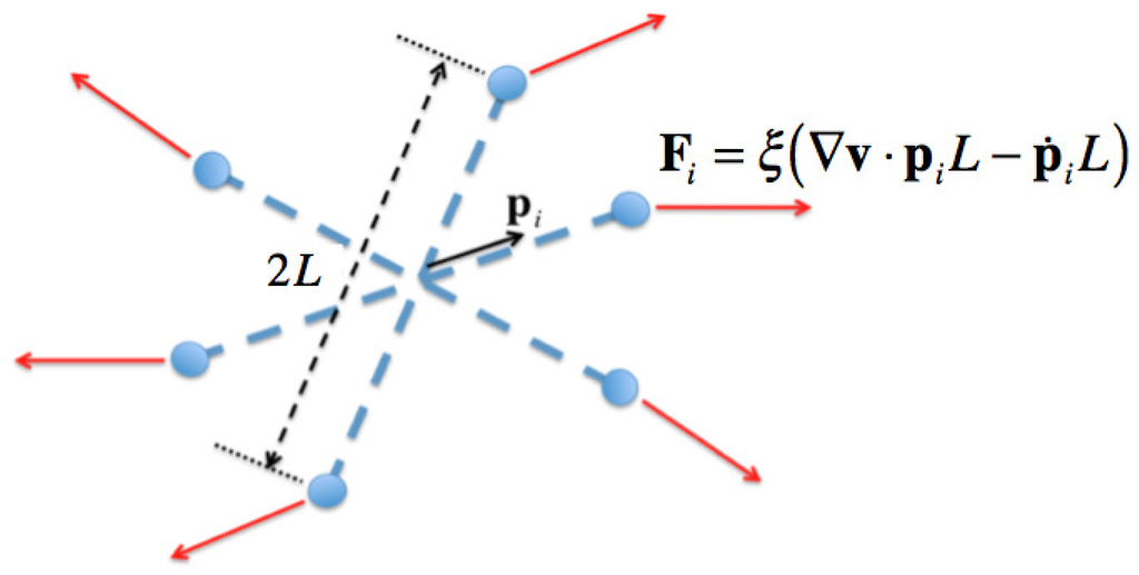
Figure 2.
Hydrodynamic forces applied on a rigid cluster composed of rods.
Remark: In this paper, we consider the following tensor products:
- if and are first rank tensors, then the single contraction, “·”, reads (Einstein summation convention);
- if and are first rank tensors, then the dyadic product,“⊗”, reads ;
- if and are first rank tensors, then the cross product, “×”, reads (Einstein summation convention) with , the components of the Levi-Civita tensor, (also known as the permutation tensor);
- if and are, respectively, second and first rank tensors, then the single contraction, “·” reads (Einstein summation convention);
- if and are second rank tensors, then the single contraction, “·”, reads (Einstein summation convention);
- if and are second rank tensors, then the double contraction, “:” reads (Einstein summation convention).
The moment induced by forces applied on rod i is given by:
By neglecting inertia effects, the resulting moment for the whole cluster must vanish:
then, taking into account Equations (1) and (2) results in:
If we define the cluster angular velocity, , such that:
in the 2D case, where and are orthogonal, , and then, it results that:
Thus, the kinematics of the rigid 2D cluster can be defined from:
the angular velocity of each rod being j:
when the cluster contains many rods, an alternative description consists of defining its orientation distribution, . In this case, all the sums in the previous expressions must be substituted by the corresponding integrals weighted with the distribution function, ψ. Thus, in the 2D case, Equation (7) leads to:
where denotes the unit sphere surface. The angular velocity of any rod, , reads:
Cross products can be written in a more compact form by using the third order Levi-Civita permutation tensor, , that allows writing using the notation previously introduced, (Einstein summation convention) or . Thus, Equation (9) writes:
with , the second moment of the orientation distribution, :
where, for the sake of notational simplicity, we do not explicate the time dependence of the distribution function, ψ.
On the other hand, we can define the rotation tensor, , such that:
that allows writing:
It is easy to prove from Equations (11)–(14) [28] that:
where and Ω are, respectively, the symmetric and skew-symmetric components of the velocity gradient, .
Thus, a rigid cluster rotates with a velocity that only depends on the second moment of its orientation distribution, . Any rigid cluster having the same orientation tensor, , will have the same angular velocity. In this case, we should derive an expression given the time evolution of , . For this purpose, we start from the definition of in Equation (12) and consider its time derivative:
where the fact that the time derivative of ψ vanishing is used. Now, taking into account Equation (14), it results that:
It is easy to prove the objectivity of expression (17) that corresponds to the Jauma’s convective derivative, as well as its null trace, i.e., [28].
3. Micro-Mechanical Description of the Kinematics of Deformable Clusters
In this section, we are considering a more realistic scenario consisting in deformable clusters. We consider two types of forces applying on each bead, one due to the fluid-rod friction, once more modeled from:
where the superscript, , refers to its hydrodynamic nature and the other , due to the rods entanglements. This last force is assumed scaling with the difference between the rigid motion velocity (the one that the bead would have if the cluster would be rigid) and the real one:
when μ is a large enough force, dominate the momentum balances, enforcing the cluster rotary velocity, , to each rod composing it (rigid behavior).
By adding both forces, it results that:
which can be rewritten as:
Now, if we define the equivalent traceless gradient, :
We can generalize all the results obtained for suspensions of dilute rods, by considering an equivalent friction coefficient, , and an equivalent gradient of velocities, . In particular, the rod rotary velocity results in:
The term deserves some additional comment. Both and Ω being skew-symmetric, it results that: and the same in the case of considering Ω, implying , and then:
which can be rewritten as:
where represents the hydrodynamic contribution in the absence of rod-rod interactions (dilute regime described by the Jeffery’s equation) and , the one coming from the rods’ entanglements, which results in a rigid-like cluster kinematics.
We can notice that when , hydrodynamic effects are preponderant, and the rod kinematics is governed by Jeffery’s equation, i.e., . In the opposite case, , the cluster is too rigid, and the rods adopt the velocity dictated by the rigid cluster kinematics, .
If we assume the orientation of the rods of a deformable cluster given by the orientation distribution, , the time derivative of its second order moment, results in:
By considering the expression of the microscopic velocity, :
it results that:
with and being the resulting expressions when Equation (27) is introduced into Equation (26) by assuming and , respectively:
with being the fourth order moment defined by:
The objectivity of the resulting evolution equation of was proven in [28]. Usually, the fourth order moment, , is expressed from the second order one by considering any of the numerous closure relations proposed in the literature [31,32,33,34]. We do not address this issue here, and from now on, we consider that , with , an appropriate algebraic operator.
Until now, the deformation mechanisms considered were purely viscous; however, it seems natural that the cluster can experience a elastic deformation with a fading-memory, that is, the reference configuration is a combination of the recent experienced deformations.
3.1. Fading Elasticity
Clusters immersed in a flowing suspension experience two types of transformations, a rigid-like one associated with rigid translations and rotations and a second one implying the cluster stretching. When the cluster conformation is described from the second order moment, , of its orientation distribution, ψ, the simplest way of quantifying stretching is by evaluating its eigenvalues change. In what follows, we consider that clusters try to recover a configuration that combines the recent ones by a sort of fading-memory, but only in what concerns the cluster stretching, that is, the memory does not concern the rigid movements.
We assume the orientation tensor, , known at times, . Tensor can be diagonalized according to:
The reference configuration, , that the cluster tries to recover at time, t, reads:
where the memory function, , decreases as increases, with for and:
As soon as the reference configuration at time t, , is available, the reference second order moment at time t, , can be obtained by applying:
If the characteristic time of the elastic recover is , then the equation governing the evolution of the second order tensor reads:
Memory effects disappear when θ vanishes. In this case, the memory function approaches the Dirac’s delta distribution, . Thus, the reference configuration corresponds to the present one, i.e., , implying the cancellation of the last term in Equation (28). Elasticity effects are also associated to Brownian effects, as discussed in [28,35,36], as well as to the rods’ bending [37,38].
4. Kinetic Theory Description
If we consider a microstructure consisting of a population of clusters and the kinematics of these clusters only depends on the second order moment of the orientation distribution of the rods that constitute them, the microstructure could be fully described from the clusters’ conformation distribution function, , given the fraction of clusters that at position and time t have a configuration described by , the last related to the orientation of the rods composing it, which was noted by .
This approach constitutes a two scale kinetic theory description, with the coarsest scale described by Ψ, depending on tensor and tensor at the finest scale depending on the rods’ orientation distribution .
Function is subjected locally (at each position, , and time t) to the normality condition:
5. Introducing Interaction Mechanisms
In concentrated regimes, clusters interact, modifying their configuration. We can distinguish two limit cases, the ones associated with soft and rigid clusters. Here, we do not consider the aggregation and breaking mechanisms that were addressed in [25,28].
5.1. Soft Clusters
In the case of soft clusters, we can expect that the orientation configuration tends to reach an isotropic distribution, i.e., in 2D. The second order moment related to such an isotropic distribution results in , where denotes the unit tensor, , with δ, the Kronecker’s delta. This fact implies that the clusters’ conformation distribution should evolve towards a Dirac distribution, i.e., .
This mechanism could be modeled by introducing a kind of collision term, , in the right-hand member of the Fokker-Planck equation (37):
with Θ, a characteristic time depending on the flow intensity, , the last described by the second invariant of the strain rate tensor, , and, also, on the clusters’ concentration, . In the previous expression, the pre-factor, , quantifies the cluster softness.
5.2. Rigid Clusters
In the case of rigid clusters, interactions can modify the cluster orientation, but not its intrinsic orientation distribution. Thus, the second order orientation tensor can rotate, but its stretching is prevented by the cluster rigidity.
Thus, the orientation tensor can change, but their eigenvalues must remain unchanged. It is easy to verify that the eigenproblem involves the characteristic equation:
where taking into account the unit trace of tensor , , proves that all the orientation tensors having the same determinant have the same eigenvalues.
The 2D conformational domain is defined by , which represents the ball centered at point , having a radius, . By developing the determinant, , it can be noticed that the determinant is constant along the circumferences centered at point . Thus, diffusion takes place along the circumferential direction defined by , being the unit vector defining the tangent direction to the circles centered at :
The diffusive flux, , reads:
with the diffusivity tensor, , given by:
If we assume that the diffusion coefficient, , scales with the cluster aspect ratio, according to , the diffusivity tensor reads:
where will depend on the flow intensity, , and the clusters’ concentration, .
The diffusive flux given by writes:
This diffusion mechanism is introduced into the right-hand member of the Fokker-Planck Equation (37) from the contribution, :
where the pre-factor quantifies the cluster rigidity.
In the case of rigid clusters, it is easy to prove that both, advection and diffusion, operate in the circumferential direction, that is, along the circles centered at point , having a radius, . Thus, one could think that a better representation could consist of considering a more appropriate choice for the conformational coordinates, allowing a simple expression of diffusion effects. One possibility lies in the choice (in the 2D case) of λ and θ, the first being the highest eigenvalue of tensor , which takes values in , and the second one, the orientation of the principal direction related to the highest eigenvalue, . Even if such a representation seems better for representing the diffusion terms, it is not the case for describing the conformational velocities in the general case (deformable aggregates).
5.3. Diffusion in the Physical Space
Because of the clusters’ interactions, we can also expect the diffusion of the cluster distribution, Ψ, in the physical space. This flux will be noted by and will be modeled by an isotropic diffusion coefficient, , that could depend on the flow intensity, , as well as on the clusters’ concentration, ϕ:
In the non-isotropic case, it suffices to replace by the diffusion tensor, , operating in the physical space. In what follows, we are considering an isotropic diffusion in the physical space.
The diffusion mechanism is introduced into the right-hand member of the Fokker-Planck equa-tion (37) from the contribution, :
5.4. Extended Fokker-Planck Equation
6. Numerical Methods
The main issue related to kinetic theory descriptions lies in its multidimensionality, because generalized Fokker-Planck equations involve the physical coordinates (space and time) and a number of conformational coordinates describing the microstructure at the desired level of detail. Classically, the curse of dimensionality was circumvented by different ways, the most usual being:
- the solution of the stochastic counterpart. However, it is well known that the control of the statistical noise and variance reduction are the main tricky issues, making possible the calculation of the distribution moments, but making difficult the reconstruction of the distribution itself [4];
- the derivation of macroscopic approaches, sometimes purely phenomenological, other times inspired or derived from finer descriptions, but even in the last case, the use of closure approximations is generally compulsory;
- introducing a first discretization by substituting conformational coordinates by a series of populations. Thus, for example, starting from:we could introduce different populations related to particular values of : and , and describe the microstructure of each one from its distribution function, , whose evolution, after discretizing with respect to the coordinate that was substituted by the populations, , in the present case, is given by the coupled lower dimensional Fokker-Planck equations:This approach was considered in the kinetic description of systems of active particles in order to circumvent the curse of dimensionality [39]; however, as soon as the dimensionality increases, the number of populations explodes.
- the use of separated representations in order to ensure that the complexity scales linearly with the model dimensionality. This technique, introduced some years ago in [40] for steady simulations and in [41] for transient solutions, consists of expressing the unknown field as a finite sum of functional products, i.e., expressing a generic multidimensional function, , as:The interested reader can refer to [42,43,44,45,46,47,48,49,50] and the references therein for a deep analysis of this technique and its applications in computational rheology.
When the partial differential equation is purely advective, the method of particles constitutes an appealing technique for solving it. As soon as diffusion terms become dominant, separated representations can be efficiently applied. At present, the main issue related to the use of separated representations techniques for solving purely advective equations is the necessity of considering accurate stabilizations [51].
6.1. Method of Particles for Solving Advection-Dominanted Problems
This technique, deeply described in [52,53], consists in approximating the initial distribution, from , Dirac’s masses, , at each one of the positions, :
which represents a sort of approximation based on pseudo-particles, , with initial positions and conformations given by:
and whose position and conformation will be evaluated all along the flow simulation, from which the distribution will be reconstructed.
6.1.1. Advection Equation
When considering the purely advective balance equation:
the time evolution of position and conformation of each particle, , is calculated by integrating:
As the position update only depends on the velocity field, which itself only depends on the position, it can be stressed that particles, , , are following the same trajectory in the physical space, having as a departure point, .
Now, the orientation distribution at time t can be reconstructed from:
Obviously, smoother representations can be obtained by considering appropriate regularizations of the Dirac’s distribution, as the one usually performed within the SPH (Smooth Particles Hydrodynamics) framework [52,54].
When balance equations involve diffusion terms, there are two main routes based on the use of particles methods, one of a stochastic nature, the other fully deterministic.
6.1.2. Advection-Diffusion Equation
For illustrating the procedure when models involve diffusion terms, we consider the Fokker-Planck equation:
where and are two diffusive fluxes operating in the physical and conformational spaces, respectively, both modeled from a Fick’s type law:
- Within the stochastic framework diffusion, terms can be modeled from appropriate random variables within a Lagrangian or a Eulerian description, the last one known as Brownian Configurations Fields (BCF). Both approaches were considered in our former works on the solution of Fokker-Planck equations [53,55]. Within the Lagrangian stochastic framework and starting from the initial cloud of pseudo-particles, , representing the initial cluster distribution, , the simplest particles updating writes:where is the time step and both random updates, and , depend on the chosen time step (see [56] for more details and for advanced stochastic integrations).Obviously, because the random effects operate in the physical space, the particles initially located at each position, , , will follow different trajectories in the physical space along the simulation time. In order to obtain accurate enough results, we must consider a rich enough representation, that is, a large population of particles. For this purpose, we must consider large enough and . The large number of particles to be tracked seems a disadvantage of the approach at first view, but it must be noticed that the integration of each particle is completely independent of all the others, making possible the use of HPCon massive parallel computing platforms.
- The technique introduced for treating purely advective equations can be extended for considering diffusion contributions, as was described in [54], and which we revisit in what follows, within a fully deterministic approach.Equation (58) can be rewritten as:orwhere the effective velocities, and , are given by:Now, the integration schema (56) can be applied by replacing material and conformation velocities, and , by their effective counterparts, and :This fully deterministic particle description requires much less particles than its stochastic counterpart, but as noticed in Equation (63), the calculation of the effective material and conformational velocities require the derivative of the cluster distribution, Ψ, with respect to both the physical and the conformational coordinates, and for that purpose, this distribution must be reconstructed all along the simulation (at each time step), a fact that constitutes a serious drawback for its implementation in massive parallel computing platforms. Moreover, to make possible the calculation of the distribution derivatives, the Dirac’s distribution must be regularized in order to ensure its derivability.
6.1.3. Discussion
It is important to note:
- Many times, the initial configuration reduces to a very small subdomain within . For example, when the initial configuration (associated with the suspension at rest) corresponds to isotropic clusters, the cluster distribution reads, . In other cases, the initial configuration can be expressed from some configurations without needing an exhaustive approximation in the whole domain, ;
- In the case of homogeneous flows, the solution is the same everywhere in the physical domain, and the distribution becomes independent of , that is, equivalent to considering in the previous analysis;
- In the case of homogeneous flows, in absence of diffusion effects and when the initial configuration reduced to a single point, , in the conformational domain, (e.g., isotropic initial configuration), a single particle suffices for tracking the microstructure evolution, i.e., and ;
- In the case of homogeneous flows, but in the presence of diffusion effects, when the initial condition can be expressed from a single point, , in the conformational domain, , stochastic simulations need considering, , but . Random contributions will produce different trajectories, , all of them starting at the same initial configuration, ;
- In the situation described in the previous item, but when considering a deterministic particles strategy, the initial location of the particles must be perturbed slightly for locating all of them in a close neighborhood of , because when all of them are located exactly at configuration , the gradient of the smoothed distribution vanishes, and then, all the trajectories will coincide;
- If the initial configuration explores the whole domain, (that in the 3D case involves a 5D configurational domain), we are faced with the redoubtable curse of dimensionality;
- The number of particles to be considered depends on the richness of the distribution to be represented in the physical and conformational spaces throughout the simulation.
6.2. Separated Representations for Solving Diffusion-Dominated Problems
When the diffusion effects are dominant, techniques presented in the previous section become inefficient, because they require an excessive number of particles to produce accurate enough results, in particular, for reconstructing the distribution. In this case, standard mesh-based discretizations seem a better choice. However, as discussed before, mesh-based discretizations fail when addressing highly dimensional models, as is the case when addressing the solution of the previous introduced Fokker-Planck equations. In that case, separated representations seem the most appealing choice.
If we consider again the Fokker-Planck equation:
There are many separated representation choices. The most natural consists of separating time, physical and conformational spaces, i.e.:
Thus, when proceeding with the Proper Generalized Decomposition—PGD—constructor [28], we must solve on the order of N 2D or 3D (depending on the dimension of the physical space) boundary value problems—BVP—for calculating functions, , the same number of 1D initial value problems—IVP—for calculating functions, , and, finally, the same number of 2D or 5D (the number of components of tensor in the 2D or 3D case, where the symmetry and its unit trace have been taken into account) BVP for calculating functions, .
This choice has a major difficulty: the problems related to the computation of are defined in 5D in the general three-dimensional case. To circumvent this difficulty, one could imagine a fully separated representation of the configuration space according to:
In what follows, for the sake of simplicity, we focus on the 2D case in which . If we consider such a separated representation, the conformational domain results in , even if, as reported before, the real conformation domain is the ball, , with center, , and radius, . When proceeding in the extended domain, , due to the consistent physics considered, the solution vanishes in .
6.3. Hybrid Strategy
A hybrid schema can be defined by using grouped conformational coordinates, that is, in Equation (66) defined in . In 2D, problems associated with functions, , are 2D, and then, they can be solved by using any standard discretization technique, like finite elements with suitable convective stabilization when required. In the 3D case, the problems related to the calculation of functions, , are defined in 5D, and then, mesh-based discretizations fail. Full separated representations, such as the ones given in Equation (67), are the most appealing choice when diffusion dominates. However, when advection dominates, a valuable alternative consists of using a method of particles, such as the ones previously described. However, it is important noticing that methods of particles are not suitable for directly computing steady state solutions (they result from the long-time solutions). Thus, an alternative separated representation reads:
where the time is grouped with the conformational coordinates, and then, particle-based techniques can be used for computing the transient solutions, , in the conformational domain.
When performing the separated representation indicated in Equation (68), the problems to be solved for calculating functions, , do not depend on , which is equivalent to the solution of a problem in a homogenous flow. All the remarks addressed in that sense when considering the methods of particles (summarized in Section 6.1.3.) apply in the present case.
7. Validating the Micro-Mechanical Models
After having proposed the micro-mechanical model, as well as the kinetic theory description, and widely discussing its numerical treatment, it is time to validate the proposed micro-mechanical model, before employing it to describe complex microstructures involved in concentrated flowing suspensions.
First of all, we are verifying the pertinence of the micro-mechanical model from a theoretical point of view. For this purpose, we first consider two particular configurations of rigid clusters for which the exact solution is known:
- Rigid cluster composed of a single rod. In this case, the exact solution corresponds to the particularization of the Jeffery’s solution [1] for an ellipsoidal particle of infinite aspect ratio, which writes:In the case of a single rod, , whose orientation is defined by , Equation (8) reduces to:and using the vector triple product formula, , it results that:which corresponds with the Jeffery’s equation for rods.
- We are now proving that the kinematics of a rigid ellipsoidal cluster composed of rods can be described by the Jeffery solution associated with an ellipsoid.In [28], we proved that for describing non-infinite aspect ratio 2D particles, it suffices to consider a rigid system composed of two rods, aligning perpendicularly one with respect to the other, and having lengths, and , , such that the parameter, r, in the general Jeffery’s equation:which depends on the ellipsoid aspect ratio, ν (length-diameter ratio):resulting from .We proved that the kinematics of a rigid cluster only depends on the second order orientation tensor, , associated with the orientation distribution of its rods, . Moreover, because of the symmetry of , it can be diagonalized, its eigenvalues in the 2D case being and (). We can evaluate the angular velocity of the rigid cluster characterized by the distribution moment, , according to Equation (14). It is easy to prove that this velocity is exactly the one related to the Jeffery’s one for an ellipsoid of aspect ratio, .
The previous verifications prove the consistency of the micromechanical model previously elaborated and whose objectivity was also proven in [28]; however its validity for describing real physical situations needs further analyses.
For validating the micromechanical model proposed in Section 3, we are considering a direct numerical simulation consisting of a population of 500 rigid rods with a given initial orientation distribution, which evolves because of the enforced flow, as well as the interaction between the rods constituting the cluster. A dense enough cluster is needed in order to ensure rigid behaviors that need a sufficient number of contact points. Using less than 500 rods does not allow for describing rigid enough clusters. The behavior does not depend on the rod length, because the velocity gradient is assumed constant at the cluster level. The contact law is assumed viscous, and its intensity is modified for ranging from deformable to rigid clusters. For additional details on the direct simulation at the microscopic scale (at the scale of the rods), the interested readers can refer to [8,26,27] and the references therein.
Figure 3 depicts the initial isotropic configuration, where the yellow points represent the contact points at which different rods interact. Then, we enforce the simple shear flow defined by the velocity field, , and adjust the intensity of the contact viscous forces applied in the microscopic direct calculation at the contact points, which allow simulating aggregates of different softness, ranging from rigid to deformable. In all cases, during the cluster configuration evolution, the second order orientation tensor is calculated by considering the star configuration depicted in Figure 1, which results in joining the cluster center of gravity to each one of the beads that it involves.
We compare the cluster configuration from its second order orientation tensor obtained from the direct simulation and the one resulting from the model described in Section 3.
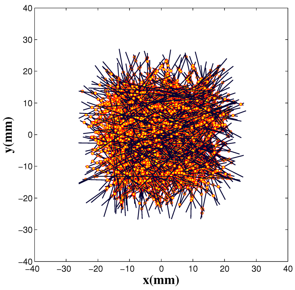
Figure 3.
Direct microscopic simulation: isotropic rods population and contact points at the initial time. A dense enough cluster ensuring many contacts between the different rods is needed in order to represent rigid enough clusters.
Figure 4, Figure 5, Figure 6, Figure 7 and Figure 8 compare model predictions versus direct simulation calculations when starting from an isotropic initial configuration for different cluster softness (ranging from very rigid to very soft). As we consider model (28), there is a single tunable parameter: , . Thus, we could consider and look for the value of μ that allows for fitting the evolution calculated from the direct simulation.
With a single tunable parameter, the comparisons allow one to conclude the excellent accuracy (qualitative and quantitative) of the proposed micromechanical model, concerning both the orientation intensity and the evolution period.
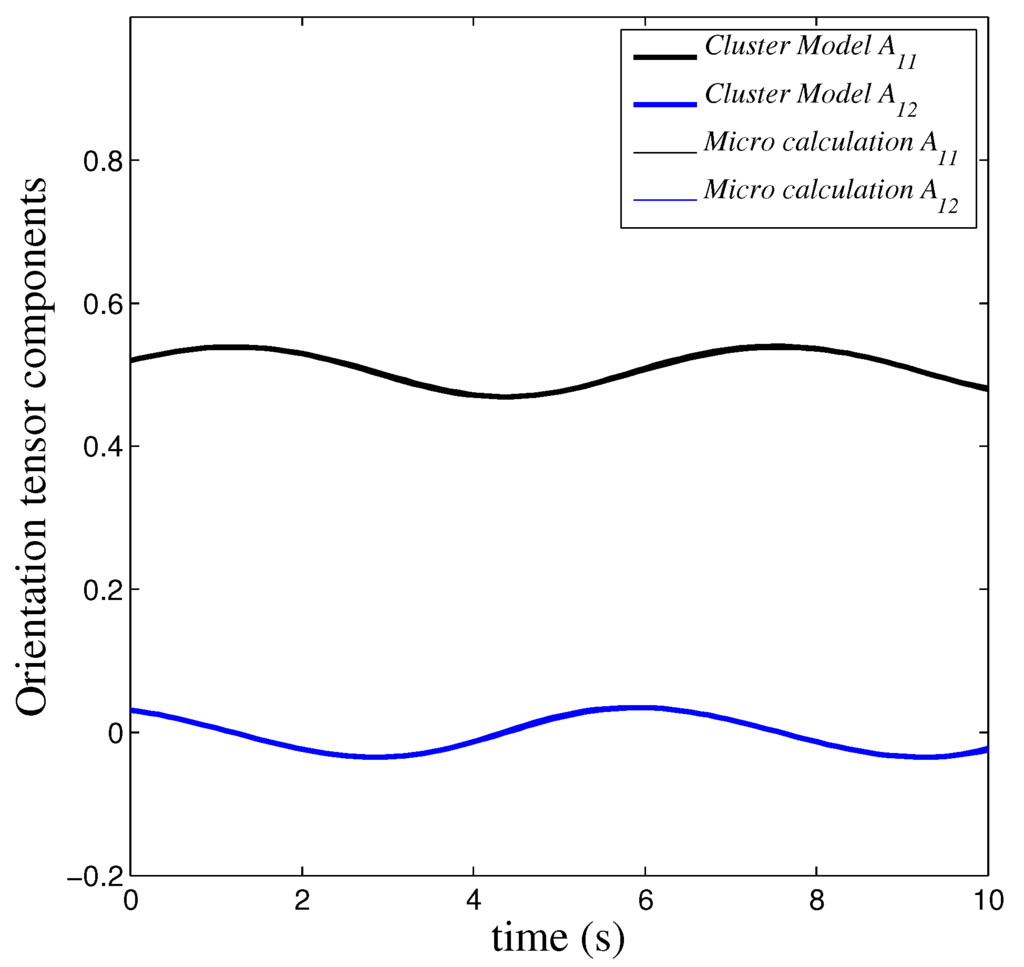
Figure 4.
Model versus direct simulation: identified .
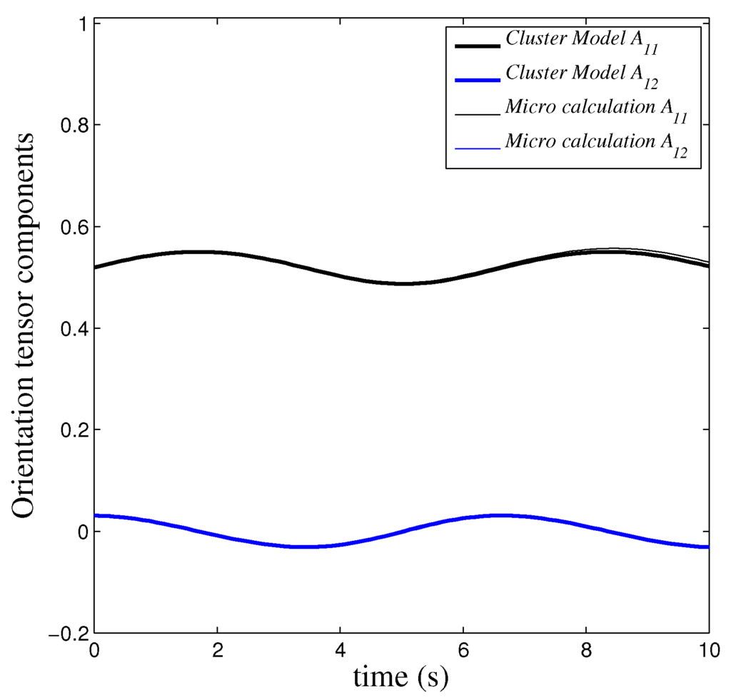
Figure 5.
Model versus direct simulation: identified .
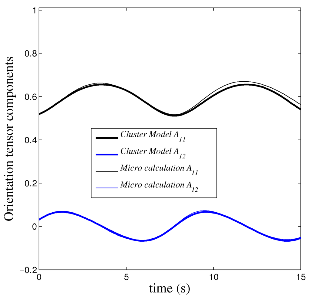
Figure 6.
Model versus direct simulation: identified .
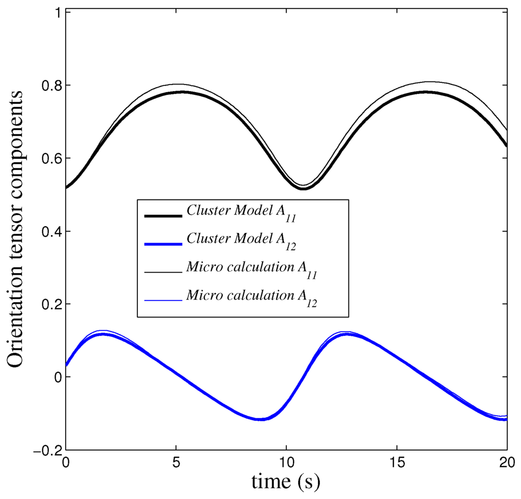
Figure 7.
Model versus direct simulation: identified .
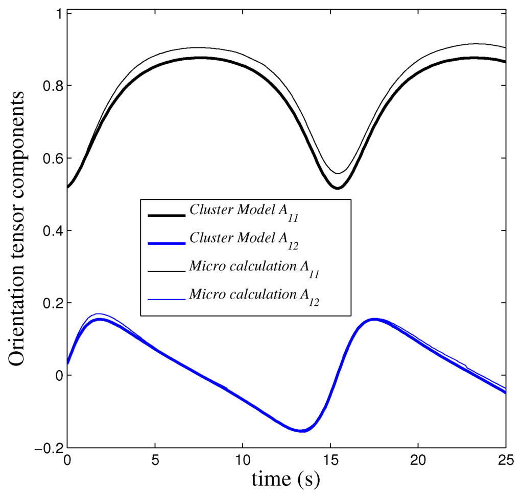
Figure 8.
Model versus direct simulation: identified .
8. Numerical Results
In this section, we are addressing preliminary results concerning the transient solution of the 2D Fokker-Planck equation (74) in a simple shear and homogeneous flow:
with , given by Equation (28) and:
for different values of and . The initial condition consists of an isotropic and normalized Gaussian distribution around the isotropic state.
Figure 9, Figure 10 and Figure 11 show the long-time cluster distributions for an effective diffusion coefficient, , and different values of the cluster softness, , and , respectively. The first corresponds almost to rigid clusters, whereas the last one corresponds to the softest ones. In the last case, we can notice that, as soon as clusters deform, they tend to align in the shear direction, , and when the deformation progresses (larger radius), clusters tend to align in the flow direction, . This mechanism is tempered by the diffusion that applies along the circumferential direction.
The previous solutions were calculated by applying a standard finite element discretization with a fine enough mesh of . When the problem is solved by considering a fully separated representation (67) in the extended conformational domain, , the solution related to rigid clusters, , involved less than 10 modes, the number of terms involved in the solution associated with the softest aggregates, , being around 40.
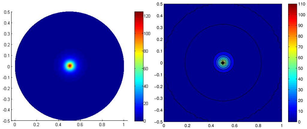
Figure 9.
Long-time cluster distribution (left) and contour levels (right), , for .

Figure 10.
Long-time cluster distribution (left) and contour levels (right) for .
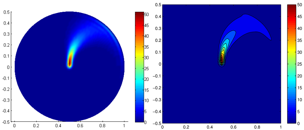
Figure 11.
Long-time cluster distribution (left) and contour levels (right), , for .
In order to point out the diffusion effects, we consider clusters with equal softness, , but subjected to different values of the effective diffusion. Figure 12 and Figure 13 show the long-time cluster distributions for effective diffusion coefficients, and , respectively. When the diffusion increases, we can notice that the flow deforms the clusters at the same time that diffusion homogenizes their orientations. For the largest diffusion, the distribution is almost uniform on the circles centered at and, consequently, the deformation mechanism seems less effective.
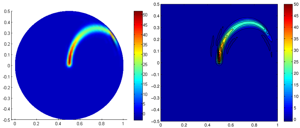
Figure 12.
Long-time cluster distribution (left) and contour levels (right), , for .
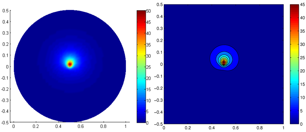
Figure 13.
Long-time cluster distribution (left) and contour levels (right), , for .
9. Conclusions
We proposed in this paper a two scale kinetic theory model of concentrated suspensions. Its main ingredients are:
- A micromechanical model describing the configuration evolution of deformable aggregates, whose kinematics only depends on the second order moment of the orientation distribution of their rods;
- The introduction of a cluster distribution that depends on the conformation of the aggregates involved in the suspension;
- The consideration of many mechanisms at both scales, the finest related to the aggregates (fading-memory elasticity) and the coarsest associated with the suspension itself, taking into account the clusters interactions.
Because the resulting kinetic theory model is defined in a highly dimensional space, the numerical strategies available for solving it were discussed deeply.
The consistency and pertinence of the micromechanical model was verified and validated by reproducing some well established results and by comparing its predictions with direct numerical simulations considering a population of rods and taking into account, explicitly, all the interactions between them.
First simulations of the kinetic theory model were finally addressed, proving the interest of the proposed approach for addressing a complex and recurrent modeling issue, the one concerning the description of rich, evolving microstructures encountered in flowing concentrated suspensions of rods.
Deeper analyses from both the modeling and the simulation point of views are in progress.
Acknowledgments
F. Chinesta acknowledges the missing symbol Institut Universitaire de France missing symbo —IUF—for its support, as well as Arnaud Poitou for the multiple and valuable discussions.
Conflict of Interest
The authors declare no conflict of interest.
References
- Jeffery, G.B. The motion of ellipsoidal particles immersed in a viscous fluid. Proc. R. Soc. Lond. 1922, A102, 161–179. [Google Scholar] [CrossRef]
- Doi, M.; Edwards, S.F. The Theory of Polymer Dynamics; Clarendon Press: Oxford, UK, 1987. [Google Scholar]
- Bird, R.B.; Crutiss, C.F.; Armstrong, R.C.; Hassager, O. Dynamic of Polymeric Liquid. In Kinetic Theory; John Wiley and Sons: Hoboken, NJ, USA, 1987; Volume 2. [Google Scholar]
- Keunings, R. Micro-macro methods for the multiscale simulation viscoelastic flow using molecular models of kinetic theory. In Rheology Reviews; Binding, D.M., Walters, K., Eds.; British Society of Rheology, 2004; pp. 67–98. [Google Scholar]
- Advani, S.; Tucker, C. The use of tensors to describe and predict fiber orientation in short fiber composites. J. Rheol. 1987, 31, 751–784. [Google Scholar] [CrossRef]
- Keunings, R. On the Peterlin approximation for finitely extensible dumbells. J. Non-Newton. Fluid Mech. 1997, 68, 85–100. [Google Scholar] [CrossRef]
- Chiba, K.; Ammar, A.; Chinesta, F. On the fiber orientation in steady recirculating flows involving short fibers suspensions. Rheol. Acta 2005, 44, 406–417. [Google Scholar] [CrossRef]
- Dumont, P.; Le Corre, S.; Orgeas, L.; Favier, D. A numerical analysis of the evolution of bundle orientation in concentrated fibre-bundle suspensions. J. Non-Newton. Fluid Mech. 2009, 160, 76–92. [Google Scholar] [CrossRef]
- Folgar, F.; Tucker, Ch. Orientation behavior of fibers in concentrated suspensions. J. Reinf. Plast. Comp. 1984, 3, 98–119. [Google Scholar] [CrossRef]
- Hand, G.L. A theory of anisotropic fluids. J. Fluid Mech. 1962, 13, 33–62. [Google Scholar] [CrossRef]
- Batchelor, G.K. The stress system in a suspension of force-free particles. J. Fluid Mech. 1970, 41, 545–570. [Google Scholar] [CrossRef]
- Hinch, J.; Leal, G. The effect of Brownian motion on the rheological properties of a suspension of non-spherical particles. J. Fluid Mech. 1972, 52, 683–712. [Google Scholar] [CrossRef]
- Hinch, J.; Leal, G. Constitutive equations in suspension mechanics. Part I. J. Fluid Mech. 1975, 71, 481–495. [Google Scholar] [CrossRef]
- Hinch, J.; Leal, G. Constitutive equations in suspension mechanics. Part II. J. Fluid Mech. 1976, 76, 187–208. [Google Scholar] [CrossRef]
- Tucker, Ch. Flow regimes for fiber suspensions in narrow gaps. J. Non-Newton. Fluid Mech. 1991, 39, 239–268. [Google Scholar] [CrossRef]
- Advani, S. Flow and Rheology in Polymer Composites Manufacturing; Elsevier: Amsterdam, The Netherlands, 1994. [Google Scholar]
- Azaiez, J.; Chiba, K.; Chinesta, F.; Poitou, A. State-of-the-art on numerical simulation of fiber-reinforced thermoplastic forming processes. Arch. Comput. Methods Eng. 2002, 9, 141–198. [Google Scholar] [CrossRef]
- Cueto, E.; Monge, R.; Chinesta, F.; Poitou, A.; Alfaro, I.; Mackley, M. Rheological modeling and forming process simulation of CNT nanocomposites. Int. J. Mater. Form. 2010, 3, 1327–1338. [Google Scholar] [CrossRef]
- Petrie, C. The rheology of fibre suspensions. J. Non-Newton. Fluid Mech. 1999, 87, 369–402. [Google Scholar] [CrossRef]
- Ma, A.; Chinesta, F.; Mackley, M. The rheology and modelling of chemically treated Carbon Nanotube suspensions. J. Rheol. 2009, 53, 547–573. [Google Scholar] [CrossRef]
- Ferec, J.; Ausias, G.; Heuzey, M.C.; Carreau, P. Modeling fiber interactions in semiconcentrated fiber suspensions. J. Rheol. 2009, 53, 49–72. [Google Scholar] [CrossRef]
- Wang, J.; Silva, C.A.; Viana, J.C.; van Hattum, F.W.J.; Cunha, A.M.; Tucker, Ch. Prediction of fiber orientation in a rotating compressing and expanding mold. Polym. Eng. Sci. 2008, 48, 1405–1413. [Google Scholar] [CrossRef]
- Wang, J.; O’Gara, J.; Tucker, C. An objective model for slow orientation kinetics in concentrated fiber suspensions: Theory and rheological evidence. J. Rheol. 2008, 52, 1179–1200. [Google Scholar] [CrossRef]
- Phelps, J.; Tucker, Ch. An anisotropic rotary diffusion model for fiber orientation in short and long fiber thermoplastics. J. Non-Newton. Fluid Mech. 2009, 156, 165–176. [Google Scholar] [CrossRef]
- Ma, A.; Chinesta, F.; Ammar, A.; Mackley, M. Rheological modelling of Carbon Nanotube aggregate suspensions. J. Rheol. 2008, 52, 1311–1330. [Google Scholar] [CrossRef]
- Le Corre, S.; Caillerie, D.; Orgéas, L.; Favier, D. Behavior of a net of fibers linked by viscous interactions: Theory and mechanical properties. J. Mech. Phys. Solids 2004, 52, 395–421. [Google Scholar] [CrossRef]
- Le Corre, S.; Dumont, P.; Orgéas, L.; Favier, D. Rheology of highly concentrated planar fiber suspensions. J. Rheol. 2005, 49, 1029–1058. [Google Scholar] [CrossRef]
- Chinesta, F. From single-scale to two-scales kinetic theory descriptions of rods suspensions. Arch. Comput. Methods Eng. 2013, 20, 1–29. [Google Scholar] [CrossRef]
- Abisset, E.; Mezher, R.; Chinesta, F. Two-scales kinetic theory model of short fibers aggregates. Key Eng. Mater. 2013, 554–557, 391–401. [Google Scholar] [CrossRef]
- Ma, A.; Chinesta, F.; Mackley, M.; Ammar, A. The rheological modelling of Carbon Nanotube (CNT) suspensions in steady shear flows. Int. J. Mater. Form. 2008, 2, 83–88. [Google Scholar] [CrossRef]
- Advani, S.; Tucker, Ch. Closure approximations for three-dimensional structure tensors. J. Rheol. 1990, 34, 367–386. [Google Scholar] [CrossRef]
- Dupret, F.; Verleye, V. Modelling the Flow of Fibre Suspensions in Narrow Gaps. In Advances in the Flow and Rheology of Non-Newton. Fluids, Rheology Series; Siginer, D.A., De Kee, D., Chabra, R.P., Eds.; Elsevier: Amsterdam, The Netherlands, 1999; pp. 1347–1398. [Google Scholar]
- Kroger, M.; Ammar, A.; Chinesta, F. Consistent closure schemes for statistical models of anisotropic fluids. J. Non-Newton. Fluid Mech. 2008, 149, 40–55. [Google Scholar] [CrossRef]
- Pruliere, E.; Ammar, A.; El Kissi, N.; Chinesta, F. Recirculating flows involving short fiber suspensions: Numerical difficulties and efficient advanced micro-macro solvers. Arch. Comput. Methods Eng. State Art Rev. 2009, 16, 1–30. [Google Scholar] [CrossRef]
- Grassia, P.; Hinch, J.; Nitsche, L.C. Computer simulations of brownian motion of complex systems. J Fluid Mech. 1995, 282, 373–403. [Google Scholar] [CrossRef]
- Grassia, P.; Hinch, J. Computer simulations of polymer chain relaxation via brownian motion. J Fluid Mech. 1996, 308, 255–288. [Google Scholar] [CrossRef]
- Cruz, C.; Illoul, L.; Chinesta, F.; Regnier, G. Effects of a bent structure on the linear viscoelastic response of Carbon Nanotube diluted suspensions. Rheol. Acta 2010, 49, 1141–1155. [Google Scholar] [CrossRef]
- Cruz, C.; Chinesta, F.; Regnier, G. Review on the Brownian dynamics simulation of bead-rod-spring models encountered in computational rheology. Arch. Comput. Methods Eng. 2012, 19, 227–259. [Google Scholar] [CrossRef]
- Bellomo, N. Modeling Complex Living Systems; Birkhauser: Boston, MA, USA, 2008. [Google Scholar]
- Ammar, A.; Mokdad, B.; Chinesta, F.; Keunings, R. A new family of solvers for some classes of multidimensional partial differential equations encountered in kinetic theory modeling of complex fluids. J. Non-Newton. Fluid Mech. 2006, 139, 153–176. [Google Scholar] [CrossRef]
- Ammar, A.; Mokdad, B.; Chinesta, F.; Keunings, R. A new family of solvers for some classes of multidimensional partial differential equations encountered in kinetic theory modeling of complex fluids. Part II: Transient simulation using space-time separated representations. J. Non-Newton. Fluid Mech. 2007, 144, 98–121. [Google Scholar] [CrossRef]
- Mokdad, B.; Pruliere, E.; Ammar, A.; Chinesta, F. On the simulation of kinetic theory models of complex fluids using the Fokker-Planck approach. Appl. Rheol. 2007, 17, 26494, 1–14. [Google Scholar]
- Leonenko, G.M.; Phillips, T.N. On the solution of the Fokker-Planck equation using a high-order reduced basis approximation. Comput. Methods Appl. Mech. Eng. 2009, 199, 158–168. [Google Scholar] [CrossRef]
- Ammar, A.; Normandin, M.; Daim, F.; Gonzalez, D.; Cueto, E.; Chinesta, F. Non-incremental strategies based on separated representations: Applications in computational rheology. Commun. Math. Sci. 2010, 8, 671–695. [Google Scholar] [CrossRef]
- Ammar, A.; Normandin, M.; Chinesta, F. Solving parametric complex fluids models in rheometric flows. J. Non-Newton. Fluid Mech. 2010, 165, 1588–1601. [Google Scholar] [CrossRef]
- Mokdad, B.; Ammar, A.; Normandin, M.; Chinesta, F.; Clermont, J.R. A fully deterministic micro-macro simulation of complex flows involving reversible network fluid models. Math. Comput. Simul. 2010, 80, 1936–1961. [Google Scholar] [CrossRef]
- Chinesta, F.; Ammar, A.; Cueto, E. Recent advances and new challenges in the use of the Proper Generalized Decomposition for solving multidimensional models. Arch. Comput. Methods Eng. 2010, 17, 327–350. [Google Scholar] [CrossRef]
- Chinesta, F.; Ammar, A.; Leygue, A.; Keunings, R. An overview of the Proper Generalized Decomposition with applications in computational rheology. J. Non-Newton. Fluid Mech. 2011, 166, 578–592. [Google Scholar] [CrossRef]
- Chinesta, F.; Ladeveze, P.; Cueto, E. A short review in model order reduction based on Proper Generalized Decomposition. Arch. Comput. Methods Eng. 2011, 18, 395–404. [Google Scholar] [CrossRef]
- Chinesta, F.; Leygue, A.; Bordeu, F.; Aguado, J.V.; Cueto, E.; Gonzalez, D.; Alfaro, I.; Ammar, A.; Huerta, A. Parametric PGD based computational vademecum for efficient design, optimization and control. Arch. Comput. Methods Eng. 2013, 20/1, 31–59. [Google Scholar] [CrossRef]
- Gonzalez, D.; Cueto, E.; Chinesta, F.; Diez, P.; Huerta, A. SUPG-based stabilization of Proper Generalized Decompositions for high-dimensional advection-diffusion equations. Int. J. Numer. Methods Eng. in press.
- Chaubal, C.; Srinivasan, A.; Egecioglu, O.; Leal, G. Smoothed particle hydrodynamics techniques for the solution of kinetic theory problems. J. Non-Newton. Fluid Mech. 1997, 70, 125–154. [Google Scholar] [CrossRef]
- Chinesta, F.; Chaidron, G.; Poitou, A. On the solution of the Fokker-Planck equation in steady recirculating flows involving short fibre suspensions. J. Non-Newton. Fluid Mech. 2003, 113, 97–125. [Google Scholar] [CrossRef]
- Ammar, A.; Chinesta, F. A Particle Strategy for Solving the Fokker-Planck Equation Governing the Fibre Orientation Distribution in Steady Recirculating Flows Involving Short Fibre Suspensions. In Lectures Notes on Computational Science and Engineering; Springer: Berlin/Heidelberg, Germany, 2005; Volume 43, pp. 1–16. [Google Scholar]
- Chinesta, F.; Ammar, A.; Falco, A.; Laso, M. On the reduction of stochastic kinetic theory models of complex fluids. Model. Simul. Mater. Sci. Eng. 2007, 15, 639–652. [Google Scholar] [CrossRef]
- Ottinger, H.C. Stochastic Processes in Polymeric Fluids; Springer: Berlin/Heidelberg, Germany, 1996. [Google Scholar]
© 2013 by the authors; licensee MDPI, Basel, Switzerland. This article is an open access article distributed under the terms and conditions of the Creative Commons Attribution license (http://creativecommons.org/licenses/by/3.0/).