Article

Statistical Properties of the Foreign Exchange Network at Different Time Scales: Evidence from Detrended Cross-Correlation Coefficient and Minimum Spanning Tree

1
College of Business Administration, Hunan University, Changsha 410082, China
2
Center of Finance and Investment Management, Hunan University, Changsha 410082, China
*
Author to whom correspondence should be addressed.
Entropy 2013, 15(5), 1643-1662; https://doi.org/10.3390/e15051643
Submission received: 15 April 2013 / Revised: 24 April 2013 / Accepted: 26 April 2013 / Published: 6 May 2013
(This article belongs to the Collection Advances in Applied Statistical Mechanics)

Abstract

:
We investigate the statistical properties of the foreign exchange (FX) network at different time scales by two approaches, namely the methods of detrended cross-correlation coefficient (DCCA coefficient) and minimum spanning tree (MST). The daily FX rates of 44 major currencies in the period of 2007–2012 are chosen as the empirical data. Based on the analysis of statistical properties of cross-correlation coefficients, we find that the cross-correlation coefficients of the FX market are fat-tailed. By examining three MSTs at three special time scales (i.e., the minimum, medium, and maximum scales), we come to some conclusions: USD and EUR are confirmed as the predominant world currencies; the Middle East cluster is very stable while the Asian cluster and the Latin America cluster are not stable in the MSTs; the Commonwealth cluster is also found in the MSTs. By studying four evaluation criteria, we find that the MSTs of the FX market present diverse topological and statistical properties at different time scales. The scale-free behavior is observed in the FX network at most of time scales. We also find that most of links in the FX network survive from one time scale to the next.

1. Introduction

It has been a “stylized fact” that financial markets are deemed as complex systems with a mass of interacting entities [1,2]. The existence of cross-correlations between financial units is a particularly important feature of market dynamics for financial markets [3,4,5]. The study on the behavior of the cross-correlations between financial agents that are beneficial to the optimization of the portfolio selection and the risk management of assets has been a hot topic [6,7,8,9]. From a statistical physics point of view, a variety of methods have been developed to analyze the cross-correlations between financial variables, such as correlation network-based approaches [10,11,12] (e.g., the minimum spanning tree (MST) [10], the planar maximally filtered graph (PMFG) [11], and the correlation threshold methods [12,13,14]), random matrix theory [15,16,17,18,19], and the (multi-)fractal analysis theory [20,21,22]. In particular, since Mantegna [10] first introduced the topology network tool of MST for the portfolio of stocks in the U.S. stock market, the correlation network-based methods have been widely used to quantify the cross-correlations and market properties in different financial markets [23], such as stock markets [13,14,24,25,26,27,28,29,30,31,32,33,34] and commodity markets [35].
The foreign exchange (FX) market is the largest and most liquid financial market [4] that directly or indirectly affects all other financial markets as any asset’s price is defined in form of a currency, which spurs many scholars to focus their studies on the topological structure and statistical properties of the FX network by correlation network-based approaches [23,36,37,38,39,40,41,42,43,44]. Previous works usually choose the MST method to analyze the topology of the correlation networks in financial markets due to its simplicity and robustness [25]. The applications of the MST method in the FX market can be divided into two aspects: on the one hand, the MST is used to analyze the clustering behavior of individual currencies in the international FX market and to find the predominant world currencies, such as in [37,38]; on the other hand, combined with the rolling (or moving) widows method [24,25], the dynamic MSTs were developed and applied to capture the time-varying behavior of the topology of the FX network and track the dynamic relationships between individual currencies in the FX market, especially during the financial crisis [42,43]. Generally, the aforementioned works using the MST approach were based on the Pearson correlation coefficient (PCC), which is used to represent the linear correlation between two time series that are both assumed to be stable [45]. Nevertheless, in the real world, the financial time series usually present the non-linear and non-stationary characteristics [23], e.g., the fat-tailed distribution has been a “stylized fact” in the return series [46,47]. Therefore, PCC may not be suitable to describe the cross-correlations between financial units that are non-stationary. To quantify the cross-correlations between two non-stationary time series i and j, a new detrended cross-correlation coefficient ρ i j ( s ) was developed by Zenbende [48], which is expressed in terms of the detrended fluctuation analysis (DFA) [49] and the detrended cross-correlation analysis (DCCA) [20] , where s is the time scale. An outstanding advantage of the DCCA coefficient (another expression of ρ i j ( s ) ) is that it can examine the cross-correlations between non-stationary time series at different time scales [4,45]. After that, the DCCA coefficient was widely used to investigate the cross-correlations in different fields [50,51], such as the FX market [4,52] and stock markets [45,53,54].
In this paper, we aim to combine the DCCA coefficient with the MST approach to construct the FX network at different time scales and analyze its statistical properties. That is to say, we want to answer the question of what statistical properties does the FX network have at different time scales, because to our knowledge there is no study that reports or reveals this issue. To this end, in our empirical analysis, we first choose 44 major currencies from 2007 to 2012 as the data set and select the special drawing right (SDR) as the numeraire. Next, we employ the DCCA coefficient to build the empirical cross-correlation matrices (CCM) of the 44 currencies at different time scales. Then, by using the filter method of the MST, we transform the empirical CCM into the FX network at different time scales. Finally, we investigate the FX network’s topological and statistical properties at different time scales.
The rest of the paper is structured as follows. In Section 2, we show the empirical data and the methodologies of the DCCA coefficient and MST. We construct the FX network at different time scales by the two methods and present the main empirical results and analysis in Section 3, and in Section 4 we draw some conclusions.

2. Data and Methodology

2.1. Data Set

The daily FX rates of 44 major currencies in the FX market from January 2, 2007 to December 31, 2012 are selected as the data set. Many previous works discussed the choice of the numeraire, which is a hard problem in the FX study because currencies are mutually priced and there is thus no independent numeraire [42]. Mizuno et al. [37] once indicated that the precious metals (e.g., the gold, platinum, and silver) can be considered as the numeraire for the FX rates. However, the precious metals should be rejected because of their high volatilities [42,43]. Other numeraire has also been suggested, such as the minor currency (e.g., the Turkish New Lira) by Keskin et al. [42], and the SDR by Wang et al. [4] and Jang et al. [43]. In our study, like in [4,43], we use the SDR, which is neither a currency nor a claim on the international monetary fund (IMF) but “a potential claim on the freely usable currencies of IMF members” [43], as the numeraire. The 44 currencies and the corresponding currency symbols are shown in Table 1. We obtain the FX data from the Pacific Exchange Rate Service [55] including 1506 days. Let P i ( t ) denote the daily FX rate of currency i on day t. The logarithmic return r i ( t ) of currency i on day t is defined as r i ( t ) = ln ( P i ( t ) ) ln ( P i ( t 1 ) ) . Therefore, the return of each currency has 1505 observations.
Table 1. 44 currencies and respective symbols.
ContinentCurrencySymbolContinentCurrencySymbol
AfricaEgyptian PoundEGPEuropeRomanian New LeoRON
South Africa RandZARRussian RublesRUB
AsiaChinese RenminbiCNYSwedish KronaSEK
Indian RupeeINR Swiss FrancCHF
Indonesian RupiahIDRTurkish New LiraTRY
Japanese YenJPYLatin AmericaArgentinian PesoARS
Malaysian RinggitMYRBrazilian RealBRL
Pakistani RupeePKRChilean PesosCLP
Philippines PesoPHPColombian PesoCOP
Singapore DollarSGDPanamanian BalboasPAB
South Korean WonKRWPeruvian New SolePEN
Sri Lankan RupeeLKRMexican PesoMXN
Taiwan DollarTWDVenezuelan Bolívar FuerteVEF
Thai BahtTHBMiddle EastIsraeli New ShekelILS
Vietnamese DongVNDJordanian DinarJOD
Vietnamese DongBritish PoundGBPKuwaiti DinarKWD
Czech KorunaCZKSaudi Arabian RiyalSAR
European EurosEURUnited Arab Emirates DirhamAED
Hungarian ForintHUFNorth AmericaCanadian DollarCAD
Icelandic KronaISKUS DollarUSD
Norwegian KroneNOKPacific OceanAustralian DollarAUD
Polish ZlotyPLNNew Zealand DollarNZD

2.2. Methodology

To construct the FX network at different time scales, we employ two approaches of the DCCA coefficient ρ i j ( s ) and the MST respectively proposed by Zenbende [48] and Mantegna [10]. First, we introduce the DCCA coefficient as follows:
Step 1. Consider two returns { r i ( t ) } and { r j ( t ) } of currencies i and j with the equal length L, where t = 1 , 2 , , L . Then, we calculate the “profile” of each return series and obtain two new sequences [52,56],
R i ( t ) = k = 1 t r i ( k ) r i , R j ( t ) = k = 1 t r j ( k ) r j , t = 1 , 2 , , L
where denotes the statistical average over the period studied.
Step 2. We divide the both profiles { R i ( k ) } and { R j ( k ) } into L s =int(L/ s ) non-overlapping units of the same length s. Considering that L is usually not a multiple of the time scale s, a short segment at the end of each profile may be left. To contain this segment of the sequences, we repeat the same procedure but starting from the opposite end. So we acquire 2 L s segments. In our study, we set 10 s L / 4 , and the number of s is fixed to be 30.
Step 3. For each segment v ( v = 1 , 2 , , L s , L s + 1 , , 2 L s ), we determine the local trends { R ˜ i v ( k ) } and { R ˜ j v ( k ) } by a least-squares fit of the sequences { R i ( k ) } and { R j ( k ) } , respectively. Then we obtain the detrended covariance [3,4,52,56]
f DCCA 2 ( s , v ) = 1 s t = 1 s R i ( v 1 ) s + t ( t ) R ˜ i v ( t ) R j ( v 1 ) s + t ( t ) R ˜ j v ( t )
for each segment v, v = 1 , 2 , , L s and
f DCCA 2 ( s , v ) = 1 s t = 1 s R i L ( v L s ) s + t ( t ) R ˜ i v ( t ) R j L ( v L s ) s + t ( t ) R ˜ j v ( t )
for v = L s + 1 , L s + 2 , , 2 L s .
Step 4. We calculate the detrended covariance fluctuation function F DCCA 2 ( s ) by averaging over all segments
F DCCA 2 ( s ) = 1 2 L s v = 1 2 L s f DCCA 2 ( s , v )
If R i ( k ) = R j ( k ) , F DCCA ( s ) reduces to the detrended variance function F DFA ( s ) defined in the DFA approach [49,57], i.e.,
F DFA ( s ) = 1 2 L s v = 1 2 L s f DFA 2 s , v 1 / 2
where f DFA 2 ( s , v ) = 1 / s t = 1 s R i ( v 1 ) s + t ( t ) R ˜ i v ( t ) 2 and f DFA 2 ( s , v ) = 1 / s t = 1 s R i L ( v L s ) s + t ( t ) R ˜ i v ( t ) 2 for v = 1 , 2 , , L s and v = L s + 1 , L s + 2 , , 2 L s , respectively.
Step 5. For the two returns { r i ( t ) } and { r j ( t ) } of currencies i and j, the DCCA coefficient is defined as the ratio between the detrended covariance function F DCCA 2 ( s ) of Equation (4) and two detrended variance functions F DFA ( s ) of Equation (5) [48,50,51,53], i.e.,
ρ i j ( s ) = F DCCA 2 ( s ) F DFA { r i ( t ) } ( s ) F DFA { r j ( t ) } ( s )
where ρ i j ( s ) ranges from 1 to 1. A value of ρ i j ( s ) = 1 or ρ i j ( s ) = 1 implies that the two currencies i and j are completely cross-correlated or anti cross-correlated, at the time scale s, whereas a value of ρ i j ( s ) = 0 indicates that there is no cross-correlation between the two currencies i and j [48]. Obviously, the DCCA coefficient ρ i j ( s ) is a function of the time scale s, which means that it can investigate the cross-correlations between two currencies i and j at different time scales [45].
Next, based on the DCCA coefficient, we simply describe the construction of the FX network using the MST method at different time scales. If there are N currencies of the same length L, MST is built by the N × N symmetric cross-correlation matrix C s of elements ρ i j ( s ) at the time scale s. To construct the MST network proposed by Mantegna [10], we use the metric distance d i j s between currencies i and j at time scale s, which satisfies the three axioms of the Euclidean distance. The metric distance is defined as d i j s = 2 ( 1 ρ i j ( s ) ) , where 0 d i j s 2 . Based on the N × N distance matrix D s of elements d i j s , we construct the MST for N currencies in the FX market via using the Kruskal’s algorithm [58,59]. For each time scale s, the MST network of the FX market connects the N currencies (nodes) with N 1 stronger links such that no loops are produced, i.e., the FX network is structured with the strongest cross-correlations of each currency [23].
Then, we introduce some evaluation criteria to examine the topological and statistical properties of the FX network. A simple measure of the normalized tree length (NTL) is proposed by Onnela et al. [24,25], which is used to analyze the temporal state of the financial market, and is defined by
L NTL ( s ) = 1 N 1 d i j s Θ d i j s
where Θ denotes the set of edges (or links) in the MST at the time scale s.
The average path length (APL), which can be used to measure the density of the MST network structure, is defined as the average distance of the shortest path between any two currencies i and j [32], i.e.,
L APL ( s ) = 2 N ( N 1 ) i > j N l i j s
where l i j s is denoted as the number of links in the shortest path between two nodes (currencies) i and j at the time scale s.
Jang et al. [43] and Yang et al. [32] suggested a measure, the maximum number of degrees (or links) k max , which is denoted as the number of links (or edges) of the most connected vertex in the MST. The greater k max that a vertex has, the larger influence of it on other vertexes is [32].
Onnela et al. [24,25] also introduced a measure of the mean occupation layer (MOL) to describe the spread of nodes on the MST, which also can be used to quantify the changes in the density of the MST. For the central vertex (or node) v c at the time scale s, the mean occupation layer is defined by
L MOL ( v c , s ) = 1 N i = 1 N l e v s ( v i )
where the central vertex in a tree is defined as a vertex that has the maximum degree (or links); lev s ( v i ) is the level of vertex v i with respect to the central vertex v c at the time scale s; and the level of the central vertex v c is set to be zero [23].

3. Empirical Results and Analysis

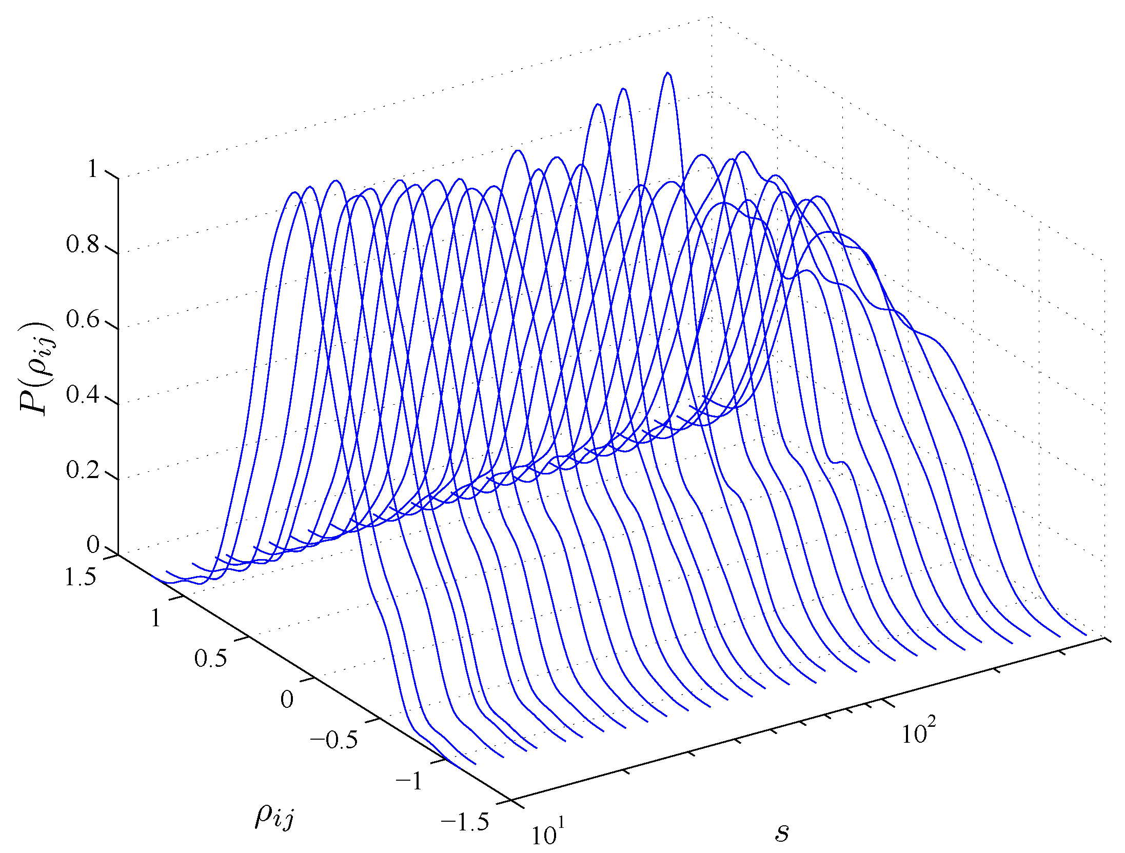
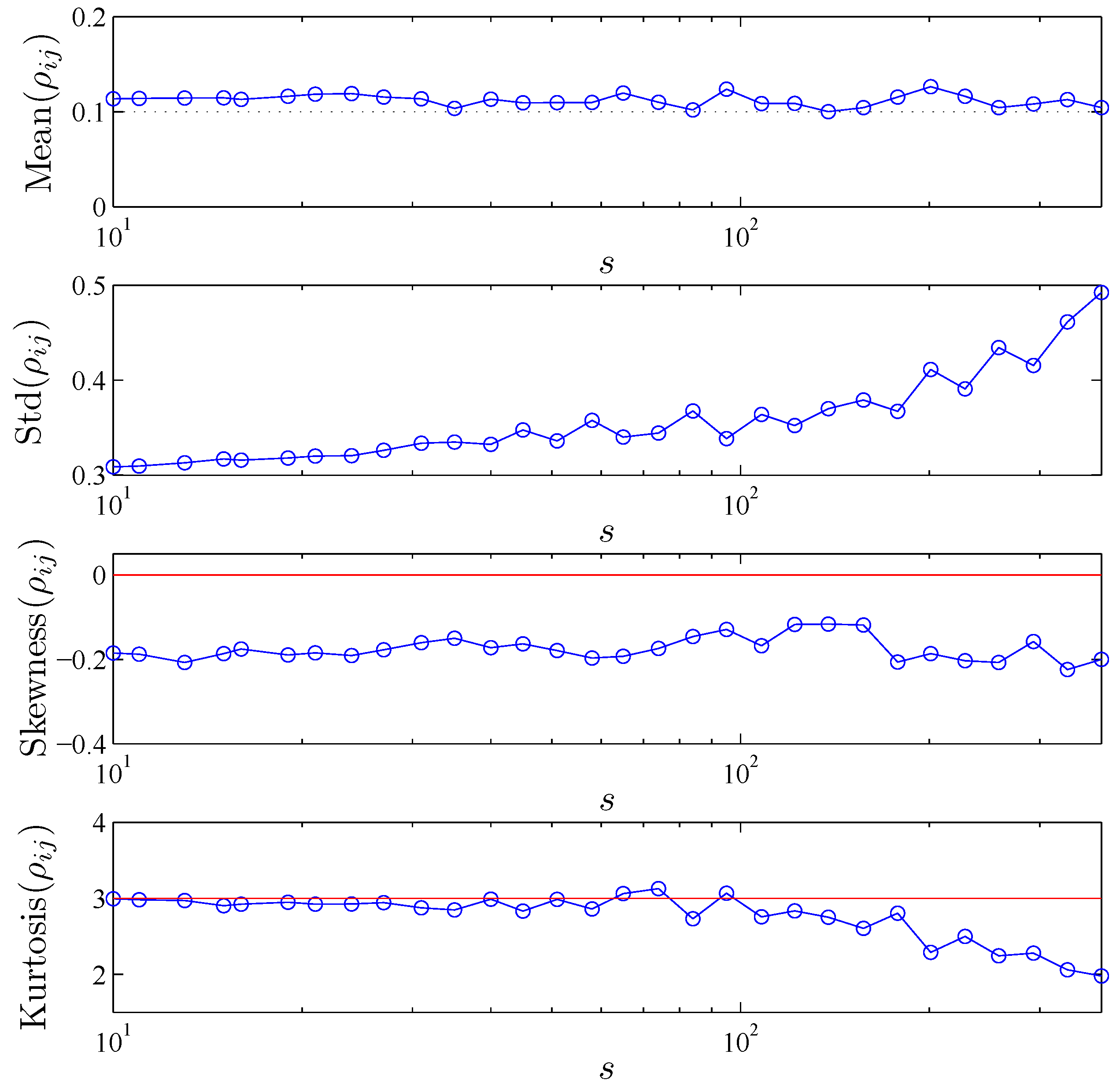
3.1. Statistics of Cross-Correlation Coefficients
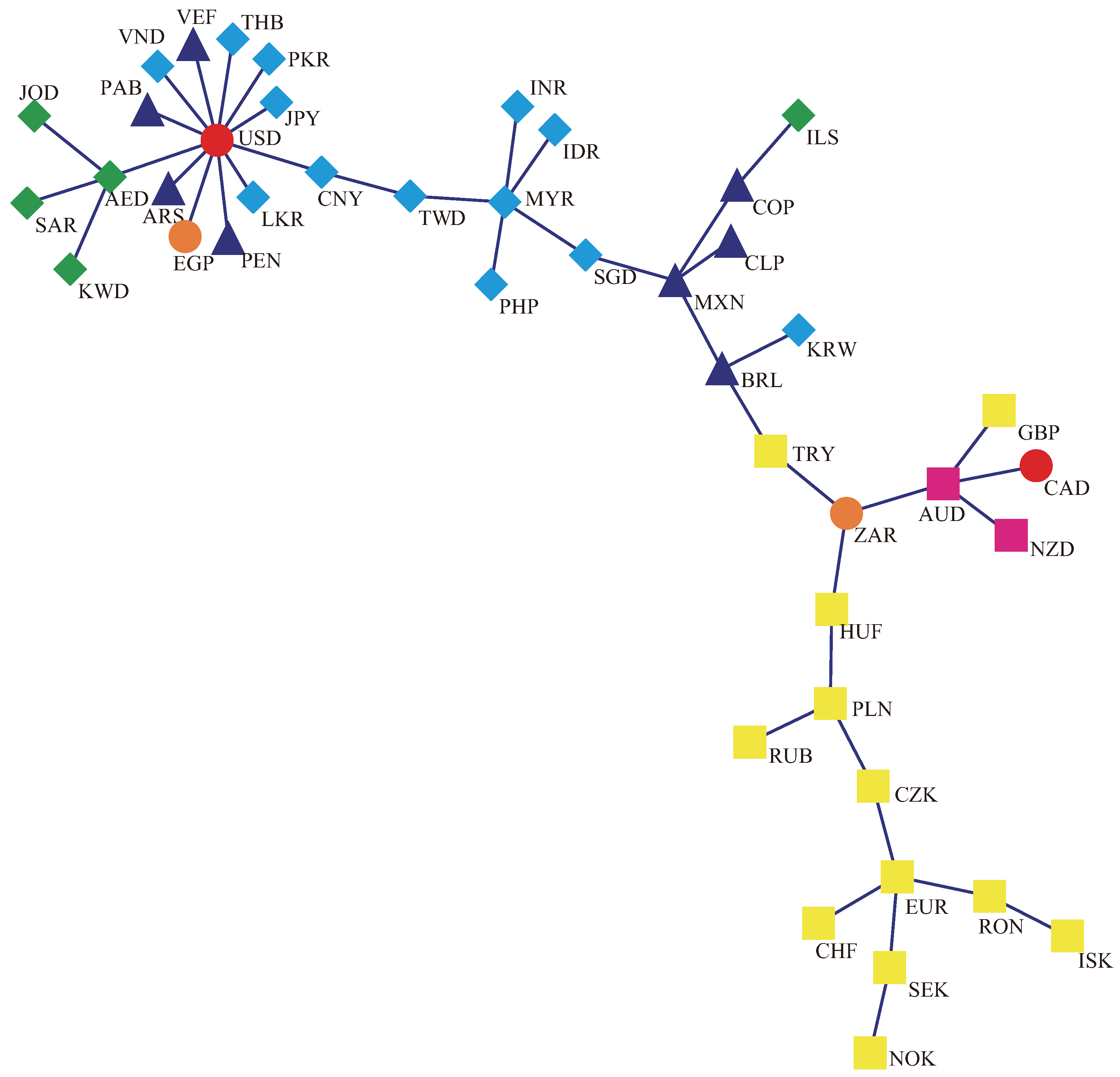
In this subsection, we investigate the probability density function (PDF) P ( ρ i j ) of the cross-correlation matrix C s with the elements { ρ i j ; i j } at the time scale s, and plot the graphical representation of P ( ρ i j ) in Figure 1. We also present four descriptive statistics (i.e., the mean, standard deviation, skewness, and kurtosis) of the cross-correlation coefficients { ρ i j ; i j } at different time scales s in Figure 2. From Figure 1 and Figure 2, for each time scale s, we can find that the PDF P ( ρ i j ) is asymmetric with a positive value as its center, in practical terms, the mean of { ρ i j ; i j } is larger than 0.1. This finding means that positive cross-correlations among the currencies in the FX market are more common than anti cross-correlations. An interesting observation in Figure 2 is that the volatility (i.e., the standard deviation) appears to increase with the time scales, which implies that the cross-correlations in the FX market seem to be unstable as the time scales increase. As shown in Figure 2, it can be found that the skewness of { ρ i j ; i j } is less than 0 and close to 0 . 2 , i.e., P ( ρ i j ) is negative skewness at each time scale s. The kurtosis of { ρ i j ; i j } is close to three, which obeys a normal distribution when s < 100, but it deviates from three and decreases with the time scales when s > 100. Based on the analysis of the skewness and kurtosis of { ρ i j ; i j } , we can conclude that the cross-correlation coefficients of the FX market in the period of 2007–2012 are fat-tailed, especially for the large time scale.
Figure 1. Plot of the probability density function P ( ρ i j ) of the cross-correlation coefficients { ρ i j ; i j } at different time scales s for the FX market in the period of 2007–2012.
Entropy 15 01643 g001
Figure 2. Plots of four descriptive statistics (i.e., the mean, standard deviation, skewness, and kurtosis) of the cross-correlation coefficients { ρ i j ; i j } at different time scales s for the FX market in the period of 2007–2012.
Entropy 15 01643 g002

3.2. MST Results

Considering that there are too many MSTs to present for all the time scales s, for the FX market, we hereby only show and analyze three MSTs at three different time scales, but in the next subsection we will present the statistical properties of the FX network at different time scales. Suppose we have s i s [ 10 , N / 4 ] , where i = 1 , 2 , . . . , 30 , the three time scales are chosen as s 1 = 10, s 15 = 58, and s 30 = 376, which are the minimum, medium, and maximum scales respectively. Figure 3, Figure 4 and Figure 5 present the MSTs of 44 currencies in the FX market during the years 2007–2012 at the three time scales s 1 = 10, s 15 = 58, and s 30 = 376, respectively.
Figure 3. Minimum spanning tree of 44 currencies in the FX market for 2007–2012 at the time scale s 1 = 10 . Coding is: Africa, orange ellipses (orange ); Asia, cyan diamonds (cyan ); Europe, yellow boxes (yellow ); Latin America, blue triangles (blue ); Middle East, green diamonds (green ); North America, red ellipses (red ); Pacific Ocean, magenta boxes (magenta ).
Entropy 15 01643 g003
For the time scale s 1 = 10, there are the two observably strongest monetary clusters in Figure 3: one is the international cluster with USD at its center, and the other is the European cluster with EUR at its center. The former is composed of some currencies directly from Asia, Latin America, Africa, and Middle East, and some currencies indirectly from Middle East and Asia. The latter is made of all the Europe currencies expect for TRY and GBP, which has typical regional or geographical feature. Possible interpretations of TRY being away from the European cluster include the marginality of the geographical position of Turkey, which is located at the border of the Europe and Asia, and that TRY is a minor currency as reported by Keskin et al. [42]. As for GBP, it is interesting to note that AUD and NZD from Pacific Ocean, CAD from North America, ZAR from Africa, and GBP from Europe are connected as the Commonwealth cluster because all the five countries come from the Commonwealth of Nations. From Figure 3, we can also find that the other three monetary clusters in the MST are the Asia cluster with MYR at its center, the Middle East cluster with AED at its center, and the Latin America cluster with MXN at its center. The former two clusters are indirectly connected with USD, which is a predominant currency in the FX market.
Figure 4. Minimum spanning tree of 44 currencies in the FX market for 2007–2012 at the time scale s 15 = 58 . Coding is: Africa, orange ellipses (orange ); Asia, cyan diamonds (cyan ); Europe, yellow boxes (yellow ); Latin America, blue triangles (blue ); Middle East, green diamonds (green ); North America, red ellipses (red ); Pacific Ocean, magenta boxes (magenta ).
Entropy 15 01643 g004
Compared with the MST in Figure 3, for the time scale s 15 = 58 as plotted in Figure 4, some changes have happened to the FX network but the two strongest monetary clusters (i.e., the international cluster and the European cluster whose centers are USD and EUR, respectively) still exist. The Asia cluster, the Middle East cluster, and the Commonwealth cluster are also presented in the graph. The biggest change is that the Latin America cluster has disappeared and the four Latin America currencies (i.e., BRL, COP, MXN, and CLP) as shown in Figure 3 are directly or indirectly linked to the Commonwealth cluster whose center is still AUD. At this time scale, the Commonwealth cluster becomes bigger than that at the time scale s 1 = 10. The positions of some currencies have also changed but it does not influence the clustering effect of the FX network.
As illustrated in Figure 5, there are several notably changes of the MST at the time scale s 30 = 376.
(1)
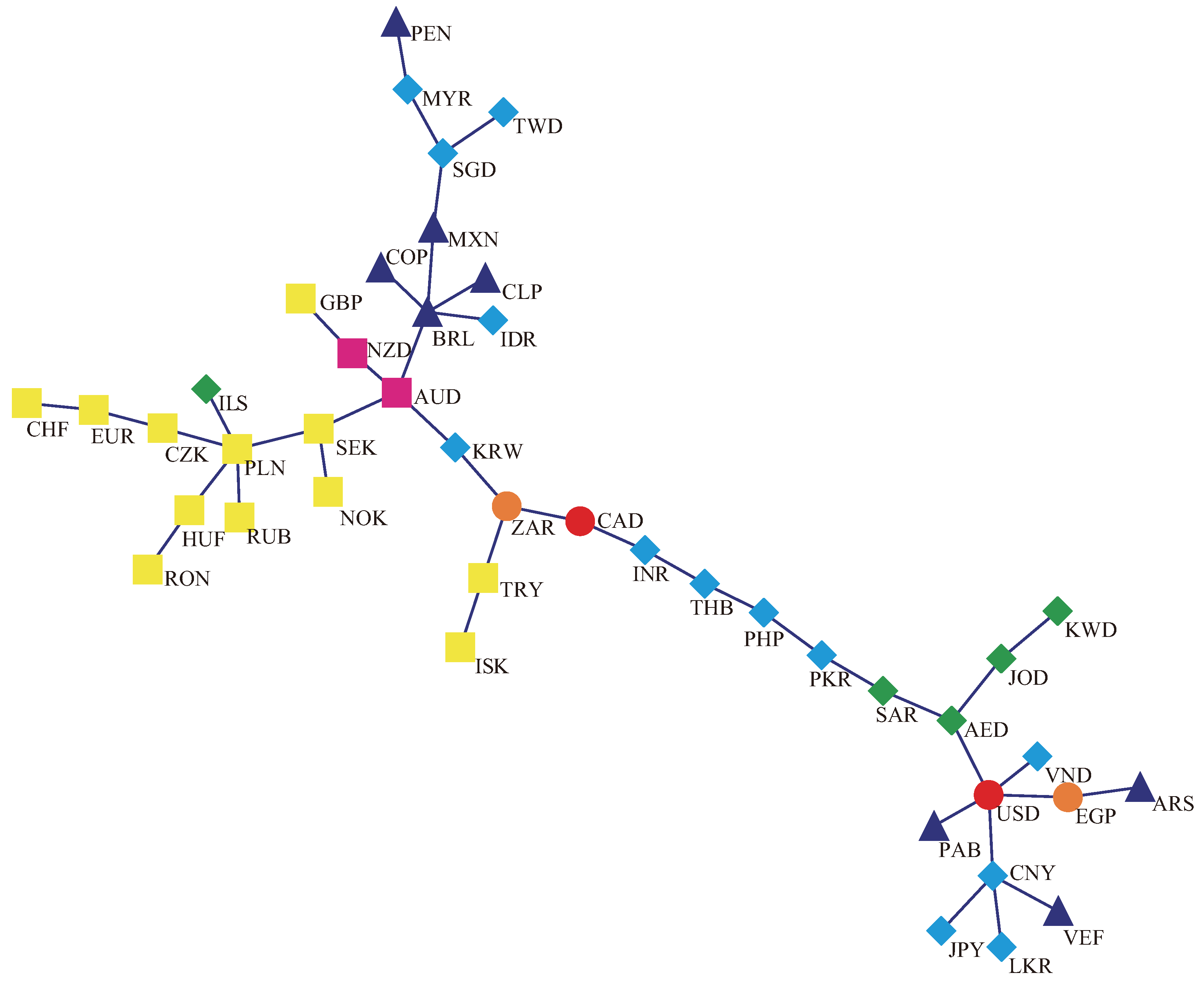
The international cluster with USD as its center becomes smaller than those of the former two scales, and only five currencies directly link to USD.
(2)
The Asia cluster splits into two small clusters: one is the linear-linked group in the MST, which is composed of INR, THB, PHP, and PKR, and the other is the triangle-linked group, which is composed of SGD, TWD, and MYR.
(3)
Compared with Figure 4, the Latin America cluster has appeared again but with BRL as its center.
(4)
Although the European cluster still exists in the MST, the center is changed to PLN.
(5)
The Commonwealth cluster is separated into two units by KRW but the five currencies (i.e., GBP, NZD, AUD, ZAR, and CAD) are still on a line.
Figure 5. Minimum spanning tree of 44 currencies in the FX market for 2007–2012 at the time scale s 30 = 376 . Coding is: Africa, orange ellipses (orange ); Asia, cyan diamonds (cyan ); Europe, yellow boxes (yellow ); Latin America, blue triangles (blue ); Middle East, green diamonds (green ); North America, red ellipses (red ); Pacific Ocean, magenta boxes (magenta ).
Entropy 15 01643 g005
From Figure 3, Figure 4 and Figure 5, we can find some similar results and draw the corresponding conclusions as follows:
(1)
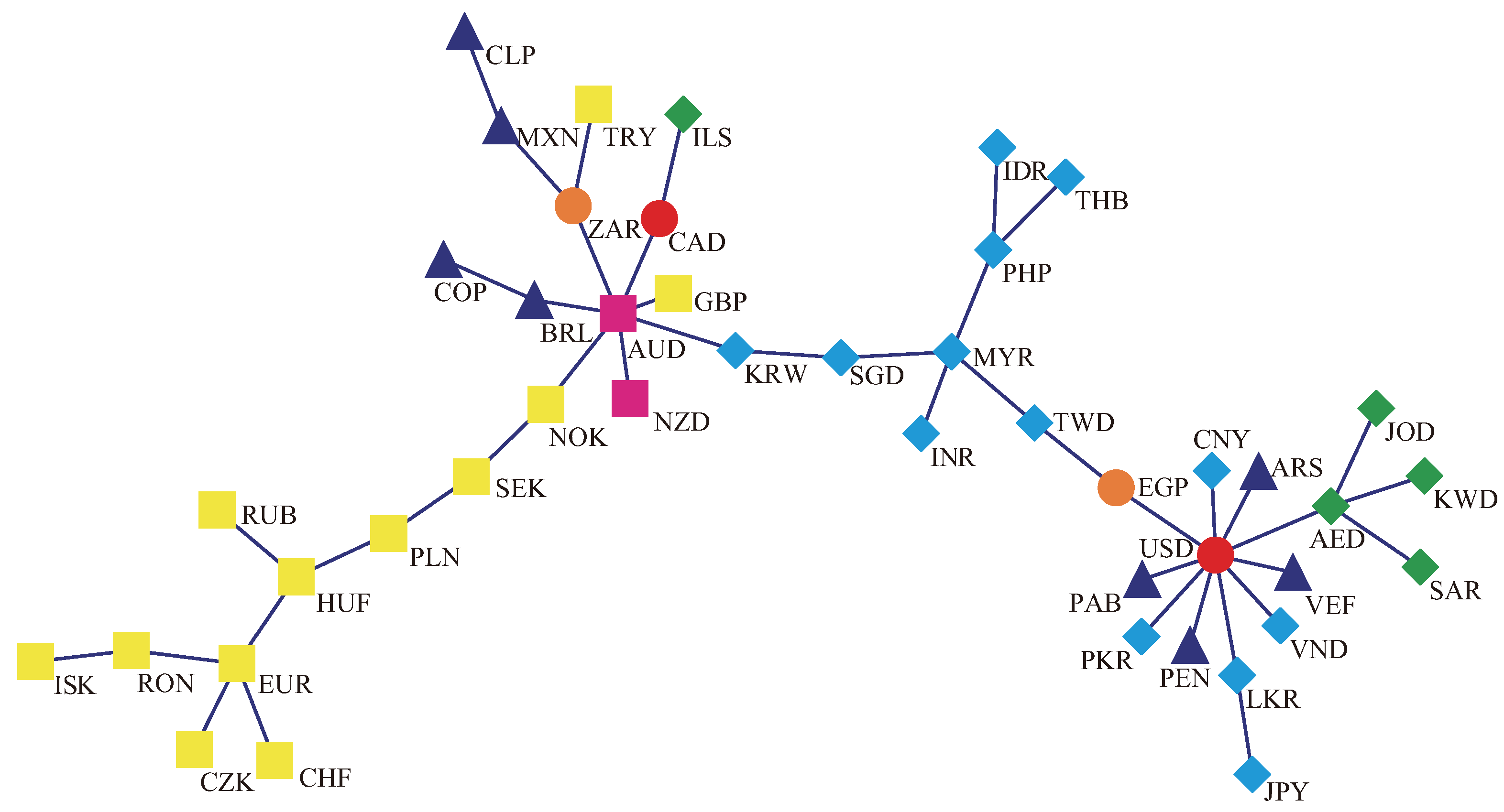
Both the international cluster and the European cluster exist in the MSTs for three different time scales, which confirms that USD and EUR are the predominant currencies in the FX market and suggests that the currencies can be clustered by the geographical criterion or the trade criterion.
(2)
Another stable cluster in the three MSTs is the Middle East cluster with AED as its center, which consists of AED, JOD, SAR, and KWD. Three countries of them are the members of the Organization of the Petroleum Exporting Countries (OPEC), which causes their currencies to have a strong relationship with USD because the U.S. is the largest importer and consumer of oil in the world at present and USD is the main currency of payment.
(3)
The Asia and Latin America clusters are not stable, which indicates that countries in these areas need more cooperation such as in the fields of trade, policy, economy, and currency.
(4)
An interesting finding is that the Commonwealth cluster appears in our study. This phenomenon suggests that the shared values and the shared trade links of the Commonwealth of Nations are beneficial to the formation of the monetary cluster.
(5)
Five currencies (i.e., CNY, PAB, VND, AED, and EGP) always connect to USD as their center. There are two possible origins to explain the connections: on the one hand, the country is one of the main trading partners of America or the opposite, such as China; on the other hand, the currency may be pegged to USD, such as PAB.
Figure 6. Plots of four evaluation criteria of MSTs at different time scales s for the FX market in the period of 2007–2012. Panels (a)–(d) show the results of L NTL , L APL , k max , and L MOL , respectively. The red solid lines represent the statistical average values over the time scales studied, corresponding to the four measures.
Entropy 15 01643 g006

3.3. Statistical Properties of MSTs at Different Time Scales

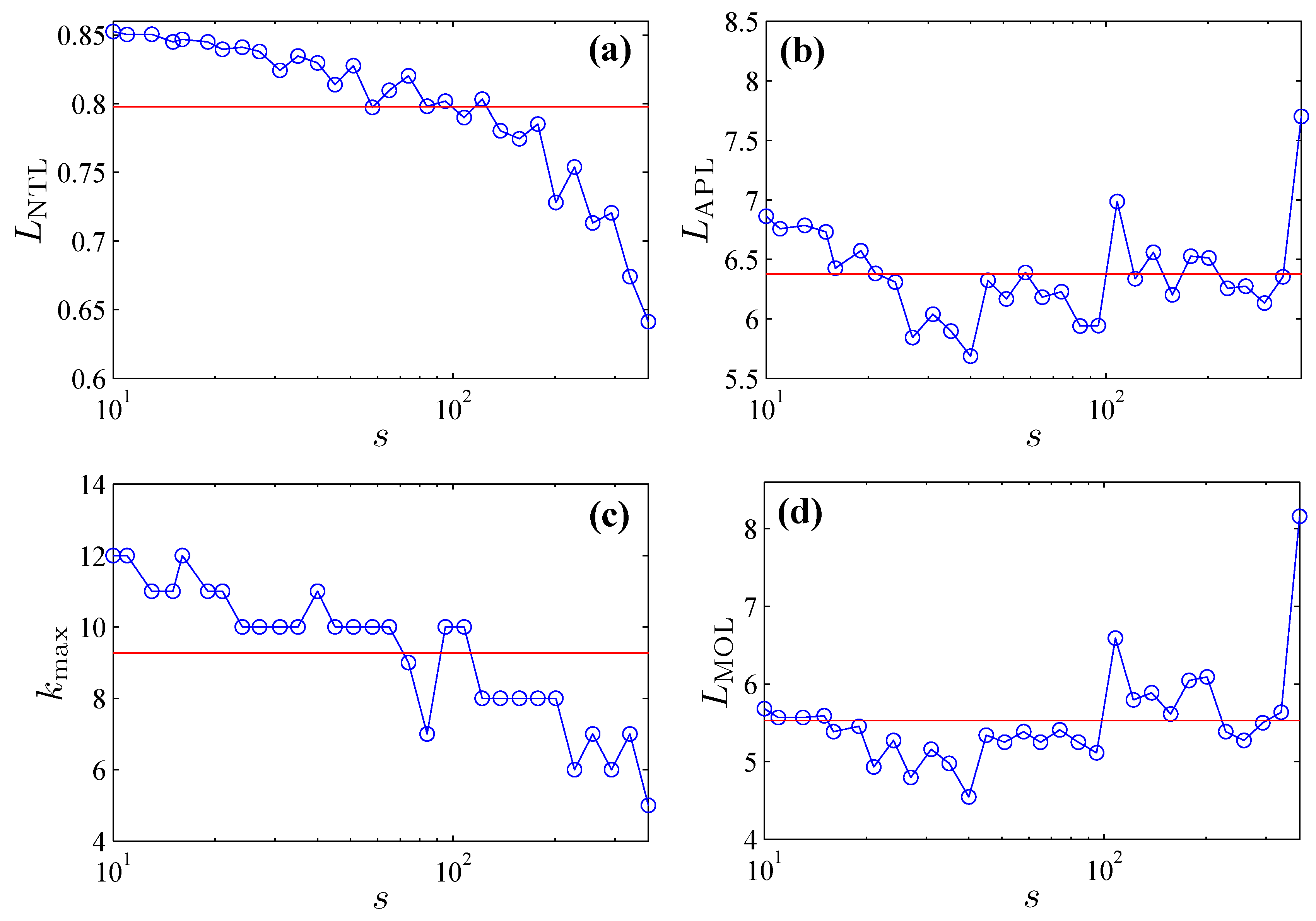
3.3.1. Four Evaluation Criteria

To analyze the topological and statistical properties of the FX network, at different time scales s, we investigate the four evaluation criteria (i.e., L NTL , L APL , k max , and L MOL ) of MSTs and show the results in Figure 6. To make a comparison, we also obtain the CCM of the 44 currencies by the method of PCC and transform the CCM into the MST for the FX market. Then, based on the MST for PCC, we calculate that the values of L NTL , L APL , k max , and L MOL are equal to 0.8672, 7.1744, 10, and 6.3409, respectively, which are all larger than the statistical average values over the time scales corresponding to the four measures of the MSTs for the DCCA coefficient (see Figure 6). As drawn in Figure 6, it can be found that all the values of L NTL , most of values of L APL and L MOL of the MSTs for the DCCA coefficient are smaller than the corresponding results of the MST for PCC. Interestingly, as shown in Figure 6a, the normalized tree length L NTL decreases with the time scales s. That is to say, the larger the time scales s is, the smaller the average distance (or length) of the FX network is. As for the average path length L APL and the mean occupation layer L MOL , the two measures have a tendency to decrease when s < 40 and do not present any consistent feature when s > 40. However, one can find that the two curves of L APL and L MOL have a similar trend from Figure 6b,d. So, we calculate that the Pearson correlation coefficient between L APL and L MOL is 0.8638 at the 1% significance level, which confirms the aforesaid finding. From Figure 6c, we can find that the maximum number of links k max represents the same value at a few successive time scales but shows a descending trend on the whole as the time scales increase. For instance, as shown in Figure 3, Figure 4 and Figure 5, it can be found that the values of k max when s 1 = 10, s 15 = 58, and s 30 = 376 are equal to 12, 10, and 5 respectively, which has a decrease tendency. From the aforementioned analysis based on Figure 6, we can come to a conclusion that the MSTs of the FX market present diverse topological and statistical properties at different time scales, which is a new visual to investigate the topology and market properties of the financial networks.

3.3.2. Distribution of Vertex Degrees

The power-law (or scale-free) behavior has been found in many financial networks [25,40,44,60]. For example, Vandewall et al. [60] investigated the vertex degrees distribution of the MST for 6358 U.S. stocks traded at the NYSE, NASDAQ, and AMEX during the year 1999 and found that the scale-free behavior exist in the stock tree. As for the definition of the scale-free behavior, Vandewall et al. [60] proposed that the probability distribution of the vertex degrees P ( k ) obeys a power-law, i.e.,
P ( k ) k α
where k is the vertex degree, and α is the exponent and is found to be 2.2 by Vandewall et al. [60]. A similar result was obtained by Onnela et al. [25] who examined the dynamic asset trees for 477 stocks traded at the NYSE from 1980 to 1999. They reported that the exponent α 2.1 for most of time but α 1.8 during the period of Black Monday. Kwapień et al. [40] investigated a set of FX rates of 63 currencies (including 3 precious metals) in the period of 1999–2008 and built different MSTs of the FX market by using different numeraires. They found that the exponents of cumulative distribution functions (CDF) are in the range [1.37, 1.96]. Because there is a difference of unity between the exponent of CDF and the exponent of the probability distribution, the exponents of the probability distribution in [40] should be in the interval [2.37, 2.96]. In other words, different MSTs based on different numeraires present different power-law exponents. From the previous works [25,40,60], we can find that the scale-free behavior of the FX market is different from that of stock markets due to the particularity of the FX market. In order to detect the power-law or scale-free behavior of MSTs for the FX market at different time scales, we introduce and employ a powerful toolbox proposed by Clauset et al. [61], which is based on the maximum likelihood estimator (MLE) and the Kolmogorov–Smirnov (KS) statistic. The probability distribution P ( k ) of the power-law model is defined by [61]
P ( k ) = α 1 k min k k min α
and the power-law exponent α is estimated by MLE, i.e.,
α ^ = 1 + N i = 1 N ln k i k min
where { k i | i =1,2,…,N} is the set of independent observations (which stand for the vertex degrees, in our study) with the elements k i such that k i k min . k min is the lower bound on the power-law behavior, which is estimated by choosing the value of k i such that KS statistic is the smallest, i.e., minimizing the KS statistic [32,
D = max k k min S ( k ) C ( k )
where S ( k ) and C ( k ) are the cumulative distribution functions of the data for the observations with value at least k min and for the power-law model that best fits the data in the region k k min [61], respectively. Based on the KS statistic, a test of p-value, which can be used to calculate a probability that the data for the observations come from the hypothesized power-law distribution [32], was proposed in [61]. If the estimated p-value is smaller than a certain chosen threshold, the power-paw hypothesis should be rejected. Similar to Clauset et al. [61], in this study, we reject the power-law model if the estimated p-value is less than 0.1. Moreover, if the estimated p-value is closer to 1, the data for the observations are more likely to draw from a power-law distribution.
Figure 7. Plots of the exponents α and the corresponding p-values of MSTs at different time scales s for the FX market in the period of 2007–2012. Panels (a) and (b) show the results of α and p-value, respectively. The red solid lines represent the statistical average values over the time scales studied, corresponding to the two measures. The black dashed line in panel (b) stands for the value of 0.1.
Entropy 15 01643 g007
Using the abovementioned method proposed by Clauset et al. [61], we estimate the exponents α and the corresponding p-values of MSTs at different time scales s for the FX market during 2007–2012, and present the results in Figure 7. From Figure 7a, we can find that the exponents are in the interval [ 2 . 12 , 3 . 50 ] and calculate their mean as 2.69, which are consistent with the results reported by Kwapień et al. [40]. About 1/3 of the exponents are in the range [ 2 . 12 , 2 . 19 ] , which are close to 2.1 obtained by Onnela et al. [25]. The rest 2/3 of the exponents fall in the interval [ 2 . 71 , 3 . 50 ] , which are much larger than the average exponent. However, as drawn in Figure 7b, it can be observed that some p-values are smaller than 0.1, which suggests that the distributions of vertex degrees for certain MSTs do not follow a power-law distribution at some time scales (i.e., s 1 , s 2 , s 3 , s 4 , s 6 , s 19 , and s 29 ). In addition, one can see that the power-law exponents of the MSTs for the FX market are different at different time scales. These findings indicate that the scale-free behavior exists in the FX network at most of time scales. As a comparison, we also estimate that the power-law exponent of the MST for PCC is equal to 3.5 and the corresponding p-value reaches to 0.751, which further confirms that scale-free behavior exists in the FX network. For each time scale, expect for the scale of s 28 , one can observe that the exponent of the MST for the DCCA coefficient is less than the exponent for PCC.
Figure 8. Plot of the L SSR of MSTs at different time scales s ( s > 10) for the FX market in the period of 2007–2012. The red solid lines represent the statistical average value over the time scales studied.
Entropy 15 01643 g008

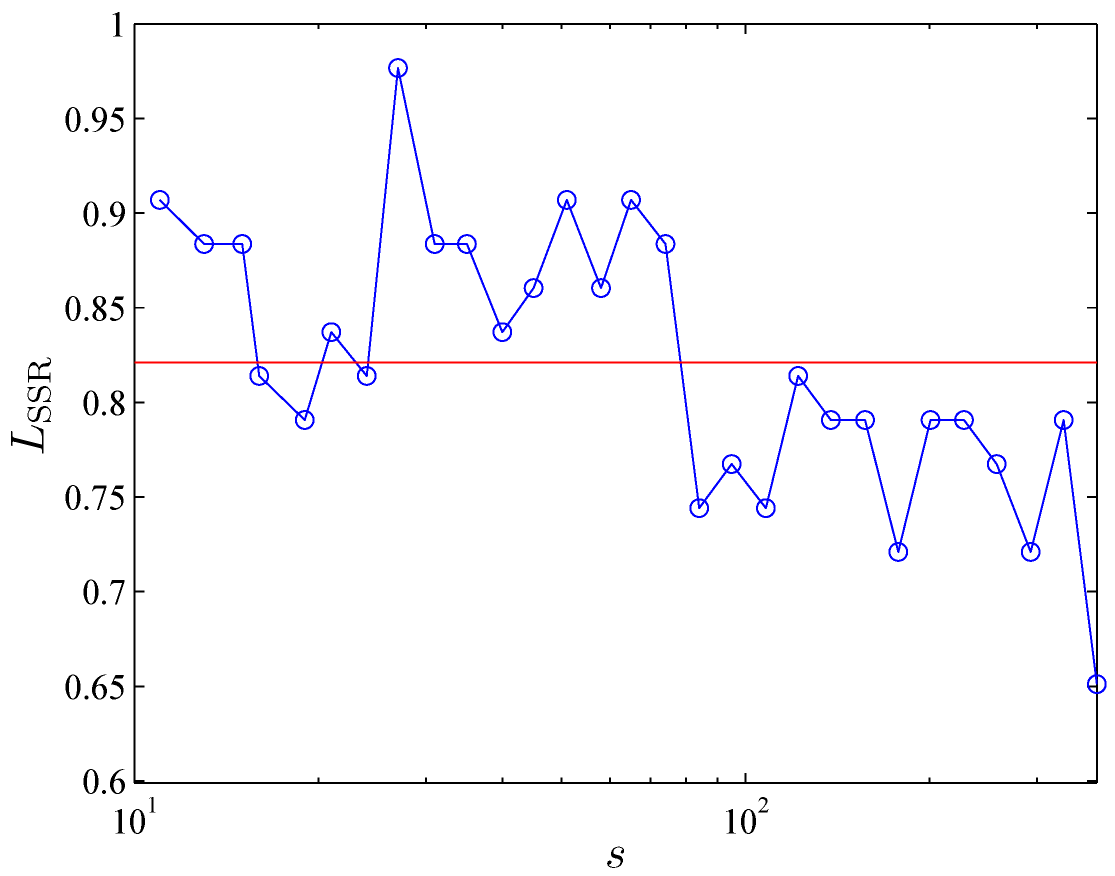
3.3.3. Single-Step Survival Ratio

Onnela et al. [24,25] defined two measures, the single-step survival ratio and the multistep survival ratio, to study the robustness and long-term evolution of the MSTs respectively. Considering that the number of time scales is limited, it is not suitable to introduce the measure of multistep survival ratio in our study. Following Onnela et al. [24,25], we hereby only introduce the single-step survival ratio (SSR), which is defined as the ratio between edges of MST and edges found in common in two consecutive MSTs at time scales s i and s i 1 , i.e., (# means the number of) [39],
L SSR ( s i ) = # E ( s i ) E ( s i 1 ) N 1
where E ( s i ) and E ( s i 1 ) stand for the set of edges of MST at time scale s i and s i 1 respectively, ∩ is the intersection operator [25], and N 1 denotes the number of edges in the MST.
We calculate the single-step survival ratio of MSTs at different time scales for the FX market by Equation (14) and show the graphical representation of L SSR in Figure 8. The average value of L SSR is equal to 0.8212, which is similar to the result reached by Onnela et al. [25] who studied the dynamic asset trees for the U.S. stock market. Moreover, there are 13/30 of L SSR larger than the average value of L SSR ; especially the maximum value reaches 0.9767, which is closes to 1. These findings imply that a great majority of links in the FX network survive from one time scale to the next. However, as a whole, the ratio decreases with increases in the time scales.

4. Conclusions

In summary, we present outcomes of this study of the FX network at different time scales based on the daily FX rates of 44 major currencies in the range from the beginning of 2007 to the end of 2012. The FX network at different time scales is constructed by two approaches, namely the methods of DCCA coefficient and MST. In the empirical process, we examine the statistical properties of cross-correlation coefficients, and three MSTs at three special time scales. We also investigate the statistical properties of MSTs for the FX market at different time scales. In practical terms, the statistical properties including four evaluation criteria (i.e., measures of the normalized tree length, the average path length, the maximum number of degrees, and the mean occupation layer), the distribution of vertex degrees, and a measure of the single-step survival ratio are analyzed.
The basic findings of the statistical properties of the FX market in our study can be summarized as follows:
(1)
Based on the analysis of statistical properties of cross-correlation coefficients, we find that the cross-correlation coefficients of the FX market in the period of 2007–2012 are fat-tailed.
(2)
From the three MSTs in Section 3.2, we draw some conclusions. For instance, USD and EUR are confirmed as the predominant world currencies in the three MSTs. The Asian cluster and the Latin America cluster are not stable while the Middle East cluster is very stable in the MSTs. It is interesting to note that the Commonwealth cluster is found in the MSTs.
(3)
By analyzing the four evaluation criteria, we find that the MSTs of the FX market present diverse topological and statistical properties at different time scales.
(4)
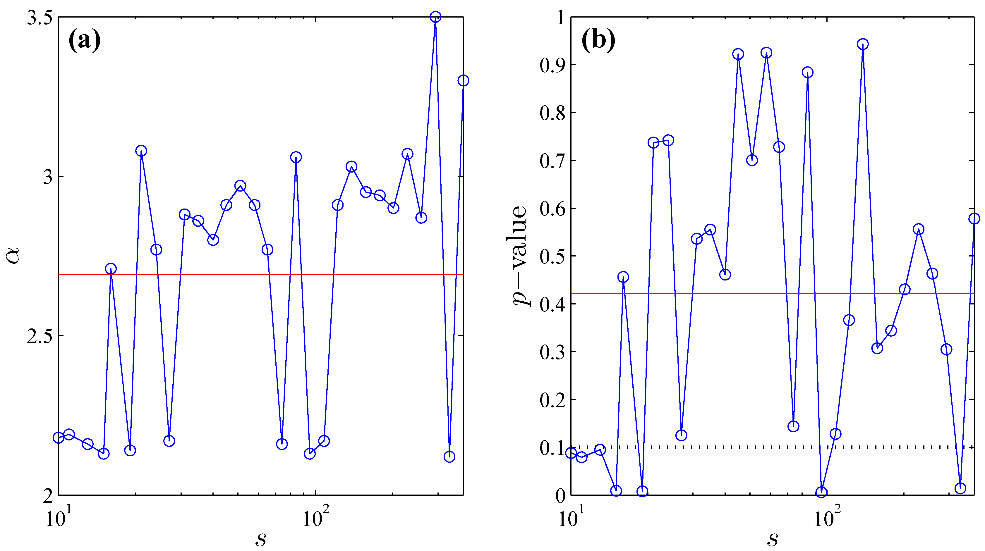
The scale-free (or power-law) behavior is also found in the FX network at most of time scales.
(5)
Through quantifying the single-step survival ratio of the MSTs at different time scales, we conclude that a great majority of links in the FX network survive from one time scale to the next.
One of the important contributions of this study is that we combine the method of DCCA coefficient with a correlation network-based method of MST to investigate the statistical properties of the FX market at different time scales. However, some open topics are not discussed in our work but can be used for the future study, which are presented as follows:
(1)
An important application of the MST is in the portfolio optimization problem, such as in [10,25]. Therefore, the different MSTs at different time scales are useful for the diversity of the asset portfolio and the optimal portfolio selection.
(2)
Our analysis based on the two methods of DCCA coefficient and MST can be employed to analyze the statistical properties of other financial markets at different time scales, such as stock markets and commodity markets.
(3)
The DCCA coefficient method also can be combined with other correlation network-based approaches to study the topology of the networks at different time scales, such as PMFG, and correlation threshold methods.

Acknowledgements

G.-J. Wang expresses thanks for the partial support from the Scholarship Award for Excellent Doctoral Student granted by the Ministry of Education of China. This work was supported by the National Social Science Foundation of China (Grant No. 07AJL005), the National Soft Science Research Program of China (Grant No. 2010GXS5B141), the Program for Changjiang Scholars and Innovative Research Team in University (Grant No. IRT0916), the Science Fund for Innovative Groups of Natural Science Foundation of Hunan Province of China (Grant No. 09JJ7002), and the Foundation for Innovative Research Groups of the National Natural Science Foundation of China (Grant No. 71221001).

References

  1. Mantegna, R.N.; Stanley, H.E. An Introduction to Econophysics: Correlations and Complexity in Finance; Cambridge University Press: Cambridge, UK, 2000. [Google Scholar]
  2. Kwapień, J.; Drożdż, S. Physical approach to complex systems. Phys. Rep. 2012, 515, 115–226. [Google Scholar] [CrossRef]
  3. Wang, G.J.; Xie, C. Cross-correlations between WTI crude oil market and US stock market: A perspective from econophysics. Acta Phys. Pol. B 2012, 43, 2021–2036. [Google Scholar] [CrossRef]
  4. Wang, G.J.; Xie, C. Cross-correlations between Renminbi and four major currencies in the Renminbi currency basket. Physica A 2013, 392, 1418–1428. [Google Scholar] [CrossRef]
  5. Kenett, D.Y.; Raddant, M.; Lux, T.; Ben-Jacob, E. Evolvement of uniformity and volatility in the stressed global financial village. PLoS One 2012, 7, e31144. [Google Scholar] [CrossRef] [PubMed]
  6. Siqueira, E.L., Jr.; Stošić, T.; Bejan, L.; Stošić, B. Correlations and cross-correlations in the Brazilian agrarian commodities and stocks. Physica A 2010, 389, 2739–2743. [Google Scholar] [CrossRef]
  7. Wang, G.J.; Xie, C. Cross-correlations between the CSI 300 spot and futures markets. Nonlinear Dyn. 2013. [Google Scholar] [CrossRef]
  8. Kenett, D.Y.; Shapira, Y.; Madi, A.; Bransburg-Zabary, S.; Gur-Gershgoren, G.; Ben-Jacob, E. Dynamics of stock market correlations. Czech AUCO Econ. Rev. 2010, 4, 330–340. [Google Scholar]
  9. Kenett, D.Y.; Preis, T.; Gur-Gershgoren, G.; Ben-Jacob, E. Quantifying meta-correlations in financial markets. Europhys. Lett. 2012, 99, 38001. [Google Scholar] [CrossRef]
  10. Mantegna, R.N. Hierarchical structure in financial markets. Eur. Phys. J. B 1999, 11, 193–197. [Google Scholar] [CrossRef]
  11. Tumminello, M.; Aste, T.; di Matteo, T.; Mantegna, R.N. A tool for filtering information in complex systems. Proc. Natl. Acad. Sci. USA 2005, 102, 10421–10426. [Google Scholar] [CrossRef] [PubMed]
  12. Boginski, V.; Butenko, S.; Pardalos, P.M. Statistical analysis of financial networks. Comput. Stat. Data Anal. 2005, 48, 431–443. [Google Scholar] [CrossRef]
  13. Huang, W.Q.; Zhuang, X.T.; Yao, S. A network analysis of the Chinese stock market. Physica A 2009, 388, 2956–2964. [Google Scholar] [CrossRef]
  14. Onnela, J.P.; Kaski, K.; Kertész, J. Clustering and information in correlation based financial networks. Eur. Phys. J. B 2004, 38, 353–362. [Google Scholar] [CrossRef]
  15. Sandoval Junior, L.; Franca, I.D.P. Correlation of financial markets in times of crisis. Physica A 2012, 391, 187–208. [Google Scholar] [CrossRef]
  16. Plerou, V.; Gopikrishnan, P.; Rosenow, B.; Amaral, L.A.N.; Guhr, T.; Stanley, H.E. Random matrix approach to cross correlations in financial data. Phys. Rev. E 2002, 65, 066126. [Google Scholar] [CrossRef] [PubMed]
  17. Laloux, L.; Cizeau, P.; Bouchaud, J.P.; Potters, M. Noise dressing of financial correlation matrices. Phys. Rev. Lett. 1999, 83, 1467–1470. [Google Scholar] [CrossRef]
  18. Plerou, V.; Gopikrishnan, P.; Rosenow, B.; Amaral, L.A.N.; Stanley, H.E. Universal and nonuniversal properties of cross correlations in financial time series. Phys. Rev. Lett. 1999, 83, 1471–1474. [Google Scholar] [CrossRef]
  19. Podobnik, B.; Wang, D.; Horvatic, D.; Grosse, I.; Stanley, H.E. Time-lag cross-correlations in collective phenomena. Europhys. Lett. 2010, 90, 68001. [Google Scholar] [CrossRef]
  20. Podobnik, B.; Stanley, H.E. Detrended cross-correlation analysis: A new method for analyzing two nonstationary time series. Phys. Rev. Lett. 2008, 100, 084102. [Google Scholar] [CrossRef] [PubMed]
  21. Zhou, W.X. Multifractal detrended cross-correlation analysis for two nonstationary signals. Phys. Rev. E 2008, 77, 066211. [Google Scholar] [CrossRef] [PubMed]
  22. Horvatic, D.; Stanley, H.E.; Podobnik, B. Detrended cross-correlation analysis for non-stationary time series with periodic trends. Europhys. Lett. 2011, 94, 18007. [Google Scholar] [CrossRef]
  23. Wang, G.J.; Xie, C.; Han, F.; Sun, B. Similarity measure and topology evolution of foreign exchange markets using dynamic time warping method: Evidence from minimal spanning tree. Physica A 2012, 391, 4136–4146. [Google Scholar] [CrossRef]
  24. Onnela, J.P.; Chakraborti, A.; Kaski, K.; Kertiész, J. Dynamic asset trees and portfolio analysis. Eur. Phys. J. B 2002, 30, 285–288. [Google Scholar] [CrossRef]
  25. Onnela, J.P.; Chakraborti, A.; Kaski, K.; Kertesz, J.; Kanto, A. Dynamics of market correlations: Taxonomy and portfolio analysis. Phys. Rev. E 2003, 68, 056110. [Google Scholar] [CrossRef] [PubMed]
  26. Jiang, Z.Q.; Zhou, W.X. Complex stock trading network among investors. Physica A 2010, 389, 4929–4941. [Google Scholar] [CrossRef]
  27. Tabak, B.M.; Serra, T.R.; Cajueiro, D.O. Topological properties of stock market networks: The case of Brazil. Physica A 2010, 389, 3240–3249. [Google Scholar] [CrossRef]
  28. Tumminello, M.; Lillo, F.; Mantegna, R.N. Correlation, hierarchies, and networks in financial markets. J. Econ. Behav. Organ. 2010, 75, 40–58. [Google Scholar] [CrossRef]
  29. Aste, T.; Shaw, W.; di Matteo, T. Correlation structure and dynamics in volatile markets. New J. Phys. 2010, 12, 085009. [Google Scholar] [CrossRef]
  30. Di Matteo, T.; Pozzi, F.; Aste, T. The use of dynamical networks to detect the hierarchical organization of financial market sectors. Eur. Phys. J. B 2010, 73, 3–11. [Google Scholar] [CrossRef]
  31. Gao, Y.C.; Wei, Z.W.; Wang, B.H. Dynamic evolution of financial network and its relation to economic crises. Int. J. Mod. Phys. C 2013, 24, 1350005. [Google Scholar] [CrossRef]
  32. Yang, C.; Shen, Y.; Xia, B. Evolution of Shanghai stock market based on maximal spanning trees. Mod. Phys. Lett. B 2013, 27, 1350022. [Google Scholar] [CrossRef]
  33. Kenett, D.Y.; Tumminello, M.; Madi, A.; Gur-Gershgoren, G.; Mantegna, R.N.; Ben-Jacob, E. Dominating clasp of the financial sector revealed by partial correlation analysis of the stock market. PLoS One 2010, 5, e15032. [Google Scholar] [CrossRef] [PubMed] [Green Version]
  34. Kenett, D.Y.; Preis, T.; Gur-Gershgoren, G.; Ben-Jacob, E. Dependency network and node influence: Application to the study of financial markets. Int. J. Bifurcat. Chaos. 2012, 22, 1250181. [Google Scholar] [CrossRef]
  35. Sieczka, P.; Hołyst, J.A. Correlations in commodity markets. Physica A 2009, 388, 1621–1630. [Google Scholar] [CrossRef]
  36. McDonald, M.; Suleman, O.; Williams, S.; Howison, S.; Johnson, N.F. Detecting a currency’s dominance or dependence using foreign exchange network trees. Phys. Rev. E 2005, 72, 046106. [Google Scholar] [CrossRef] [PubMed]
  37. Mizuno, T.; Takayasu, H.; Takayasu, M. Correlation networks among currencies. Physica A 2006, 364, 336–342. [Google Scholar] [CrossRef]
  38. Naylor, M.J.; Rose, L.C.; Moyle, B.J. Topology of foreign exchange markets using hierarchical structure methods. Physica A 2007, 382, 199–208. [Google Scholar] [CrossRef]
  39. Kwapień, J.; Gworek, S.; Drożdż, S. Structure and evolution of the foreign exchange networks. Acta Phys. Pol. B 2009, 40, 175–194. [Google Scholar]
  40. Kwapień, J.; Gworek, S.; Drożdż, S.; Górski, A. Analysis of a network structure of the foreign currency exchange market. J. Econ. Interact. Coord. 2009, 4, 55–72. [Google Scholar] [CrossRef]
  41. Gworek, S.; Kwapień, J.; Drożdż, S. Sign and amplitude representation of the forex networks. Acta Phys. Pol. A 2010, 117, 681–687. [Google Scholar]
  42. Keskin, M.; Deviren, B.; Kocakaplan, Y. Topology of the correlation networks among major currencies using hierarchical structure methods. Physica A 2011, 390, 719–730. [Google Scholar] [CrossRef]
  43. Jang, W.; Lee, J.; Chang, W. Currency crises and the evolution of foreign exchange market: Evidence from minimum spanning tree. Physica A 2011, 390, 707–718. [Google Scholar] [CrossRef]
  44. Górski, A.Z.; Drożdż, S.; Kwapień, J. Scale free effects in world currency exchange network. Eur. Phys. J. B 2008, 66, 91–96. [Google Scholar] [CrossRef]
  45. Gu, R.; Shao, Y.; Wang, Q. Is the efficiency of stock market correlated with multifractality? An evidence from the Shanghai stock market. Physica A 2013, 392, 361–370. [Google Scholar] [CrossRef]
  46. Mantegna, R.N.; Stanley, H.E. Scaling behaviour in the dynamics of an economic index. Nature 1995, 376, 46–46. [Google Scholar] [CrossRef]
  47. Drożdż, S.; Kwapień, J.; Oświȩcimka, P.; Rafał, R. The foreign exchange market: Return distributions, multifractality, anomalous multifractality and the Epps effect. New J. Phys. 2010, 12, 105003. [Google Scholar] [CrossRef]
  48. Zebende, G.F. DCCA cross-correlation coefficient: Quantifying level of cross-correlation. Physica A 2011, 390, 614–618. [Google Scholar] [CrossRef]
  49. Peng, C.K.; Buldyrev, S.V.; Havlin, S.; Simons, M.; Stanley, H.E.; Goldberger, A.L. Mosaic organization of DNA nucleotides. Phys. Rev. E 1994, 49, 1685–1689. [Google Scholar] [CrossRef]
  50. Vassoler, R.T.; Zebende, G.F. DCCA cross-correlation coefficient apply in time series of air temperature and air relative humidity. Physica A 2012, 391, 2438–2443. [Google Scholar] [CrossRef]
  51. Zebende, G.F.; da Silva, M.F.; Machado Filho, A. DCCA cross-correlation coefficient differentiation: Theoretical and practical approaches. Physica A 2013, 392, 1756–1761. [Google Scholar] [CrossRef]
  52. Cao, G.; Xu, L.; Cao, J. Multifractal detrended cross-correlations between the Chinese exchange market and stock market. Physica A 2012, 391, 4855–4866. [Google Scholar] [CrossRef]
  53. Podobnik, B.; Jiang, Z.Q.; Zhou, W.X.; Stanley, H.E. Statistical tests for power-law cross-correlated processes. Phys. Rev. E 2011, 84, 066118. [Google Scholar] [CrossRef] [PubMed]
  54. Wang, G.J.; Xie, C.; Chen, S.; Yang, J.J.; Yang, M.Y. Random matrix theory analysis of cross-correlations in the U.S. stock market: Evidence from Pearson correlation coefficient and detrended cross-correlation coefficient. Physica A 2013. [Google Scholar] [CrossRef]
  55. Pacific Exchange Rate Service. Available online: http://fx.sauder.ubc.ca/data.html (accessed on 6 May 2013).
  56. Wang, Y.; Wei, Y.; Wu, C. Cross-correlations between Chinese A-share and B-share markets. Physica A 2010, 389, 5468–5478. [Google Scholar] [CrossRef]
  57. Kantelhardt, J.W.; Zschiegner, S.A.; Koscielny-Bunde, E.; Havlin, S.; Bunde, A.; Stanley, H.E. Multifractal detrended fluctuation analysis of nonstationary time series. Physica A 2002, 316, 87–114. [Google Scholar] [CrossRef]
  58. Kruskal, J.B., Jr. On the shortest spanning subtree of a graph and the traveling salesman problem. Proc. Am. Math. Soc. 1956, 7, 48–50. [Google Scholar] [CrossRef]
  59. Djauhari, M.A.; Gan, S.L. Minimal spanning tree problem in stock networks analysis: An efficient algorithm. Physica A 2013, 392, 2226–2234. [Google Scholar] [CrossRef]
  60. Vandewalle, N.; Brisbois, F.; Tordoir, X. Non-random topology of stock markets. Quant. Econom. 2001, 1, 372–374. [Google Scholar] [CrossRef]
  61. Clauset, A.; Shalizi, C.R.; Newman, M.E.J. Power-law distributions in empirical data. SIAM Rev. 2009, 51, 661–703. [Google Scholar] [CrossRef]

