Article

A Free Energy Principle for Biological Systems

The Wellcome Trust Centre for Neuroimaging, Institute of Neurology, Queen Square, London, WC1N 3BG, UK
Entropy 2012, 14(11), 2100-2121; https://doi.org/10.3390/e14112100
Submission received: 17 August 2012 / Revised: 1 October 2012 / Accepted: 25 October 2012 / Published: 31 October 2012
(This article belongs to the Special Issue The Information Bottleneck Method)

Abstract

:
This paper describes a free energy principle that tries to explain the ability of biological systems to resist a natural tendency to disorder. It appeals to circular causality of the sort found in synergetic formulations of self-organization (e.g., the slaving principle) and models of coupled dynamical systems, using nonlinear Fokker Planck equations. Here, circular causality is induced by separating the states of a random dynamical system into external and internal states, where external states are subject to random fluctuations and internal states are not. This reduces the problem to finding some (deterministic) dynamics of the internal states that ensure the system visits a limited number of external states; in other words, the measure of its (random) attracting set, or the Shannon entropy of the external states is small. We motivate a solution using a principle of least action based on variational free energy (from statistical physics) and establish the conditions under which it is formally equivalent to the information bottleneck method. This approach has proved useful in understanding the functional architecture of the brain. The generality of variational free energy minimisation and corresponding information theoretic formulations may speak to interesting applications beyond the neurosciences; e.g., in molecular or evolutionary biology.
PACS Codes:
87.18.Vf, 02.70.Rr

1. Introduction

What are the basic principles that underwrite the self-organisation or self-assembly of biological systems like cells, plants and brains? This paper tries to address this question by asking how a biological system, exposed to random and unpredictable fluctuations in its external milieu, can restrict itself to occupying a limited number of states, and therefore survive in some recognisable form. The answer we entertain is based upon a variational free energy minimisation principle that has proved useful in accounting for many aspects of brain structure and function. In brief, biological systems can distil structural regularities from environmental fluctuations (like changing concentrations of chemical attractants or sensory signals) and embody them in their form and internal dynamics. In essence, they become models of causal structure in their local environment, enabling them to predict what will happen next and counter surprising violations of those predictions. In other words, by modelling their environment they acquire a homoeostasis and can limit the number of states they find themselves in. This perspective on self-organisation is interesting because it connects probabilistic descriptions of the states occupied by biological systems to probabilistic modelling or inference as described by Bayesian probability and information theory [1,2]. This connection is exploited to interpret biological behaviour in terms of action and perception and to show that action and perception (in an abstract sense) can be found any system that resists a natural tendency to disorder. Furthermore, such systems conform to information theoretic constraints, of the sort prescribed by the information bottleneck method.
Over the past decade, a free energy principle has been proposed that explains several aspects of action, perception and cognition in the neurosciences [3]. This principle appeals to variational Bayesian methods in statistics to understand how the brain infers the causes of its sensory inputs based on the original proposal of Helmholtz [4] and subsequent advances in psychology and machine learning [5,6,7,8]. In brief, variational Bayesian methods allow one to perform approximate Bayesian inference, given some data and a (generative) model of how those data were generated. The key feature of these methods is the minimization of a variational free energy that bounds the (negative log) evidence for the model in question. This minimization eschews the difficult problem of evaluating the evidence directly [9], where evidence corresponds to the probability of some data, given the model. The underlying variational methods were introduced in the context of quantum physics by Richard Feynman [10] and have been developed by Geoffrey Hinton and others in machine learning [11,12]. These variational methods furnish efficient Bayesian procedures that are now used widely to analyze empirical data; e.g. [13]. Crucially, under some simplifying assumptions, these variational schemes can be implemented in a biologically plausible way, making them an important metaphor for neuronal processing in the brain. One popular example is predictive coding [14]. The same variational formalism has also found a powerful application in the setting of optimal control and the construction of adaptive agents. For example, Ortega and Braun [15], consider the problem of optimising active agents, where past actions need to be treated as causal interventions. They show that that the solution to this variational problem is given by a stochastic controller called the Bayesian control rule, which implements adaptive behaviour as a mixture of experts. This work illustrates the close connections between minimising (relative) entropy and the ensuing active Bayesian inference that is the focus of this paper.
Minimising variational free energy (maximising Bayesian model evidence) not only provides a principled explanation for perceptual (Bayesian) inference in the brain but can also explain action and behaviour [15,16]. This rests on noting that minimizing free energy implicitly minimizes the long-term time average of self-information (surprisal) and, under ergodic assumptions, the Shannon entropy of sensory states. The principle of variational free energy minimization has therefore been proposed to explain the ability of complex systems like the brain to resist a natural tendency to disorder and maintain a sustained and homoeostatic exchange with its environment [17]. Since that time, the free energy principle has been used to account for a variety of phenomena in sensory [18,19], cognitive [20] and motor neuroscience [21,22,23] and has provided useful insights into structure-function relationships in the brain (Table 1). Free energy formulations also provide a powerful account of optimal control beyond biological settings and can be derived axiomatically by considering the information costs and complexity of bounded rational decision-making [24]. These formulations provide an important link between information theory (in the sense of statistical thermodynamics) and general formulations of adaptive agents in terms of utility theory and optimal decision theory.
In what follows, we motivate the free energy principle in general (and abstract) terms―using random dynamical systems and information theory, starting with the premise that biological agents resist a dispersion of their states in the face of fluctuations in the environment. We presume that this characterizes open biological systems that exhibit homoeostasis (from Greek: ὅμοιος, hómoios, similar and στάσις, stásis, standing still) – in other words, systems that maintain their states within certain bounds [17,25,26,27,28,29,30] Using minimal assumptions, we show that this sort of behaviour can be cast in terms of Bayesian modelling of causal structure in the environment; in a way that is consistent with both the good regulator theorem (every Good Regulator of a system must be a model of that system [31]) and Jaynesian perspectives on statistical physics [32]. Having established that variational free energy minimization is a sufficient account of self-organising behaviour, we then consider this behaviour in terms of information theory, in particular the information bottleneck criterion. We conclude by illustrating the implications of the theoretical arguments with a neurobiological example. This example focuses on perception in the brain, to show how it informs the functional architecture of brain circuits.
Table 1. Processes and paradigms that have been modelled using the scheme in this paper.
DomainProcess or paradigm
Perception
Perceptual categorisation (bird songs) [18]
Novelty and omission-related responses [18]
Perceptual inference (speech) [19]
Sensory learning
Perceptual learning (mismatch negativity) [33]
Attention
Attention and the Posner paradigm [20]
Attention and biased competition [20]
Motor control
Retinal stabilization and oculomotor reflexes [21]
Saccadic eye movements and cued reaching [21]
Motor trajectories and place cells [22]
Sensorimotor integration
Bayes-optimal sensorimotor integration [21]
Behaviour
Heuristics and dynamical systems theory [23]
Goal-directed behaviour [23]
Action observation
Action observation and mirror neurons [22]

2. Entropy and Random Dynamical Attractors

The problem addressed in this section is how low-entropy probability distributions over states are maintained, when systems are immersed in a changing environment [17]. In particular, how do (biological) systems resist the dispersive effects of fluctuations in their external milieu? We reduce this problem to finding a deterministic mapping among the physical states of the system that ensures they occupy a small number of attracting states. In the following, we describe the sort of behaviour that we are trying to explain and consider a solution based on the principle of least (stationary) action.

2.1. Setup and Preliminaries
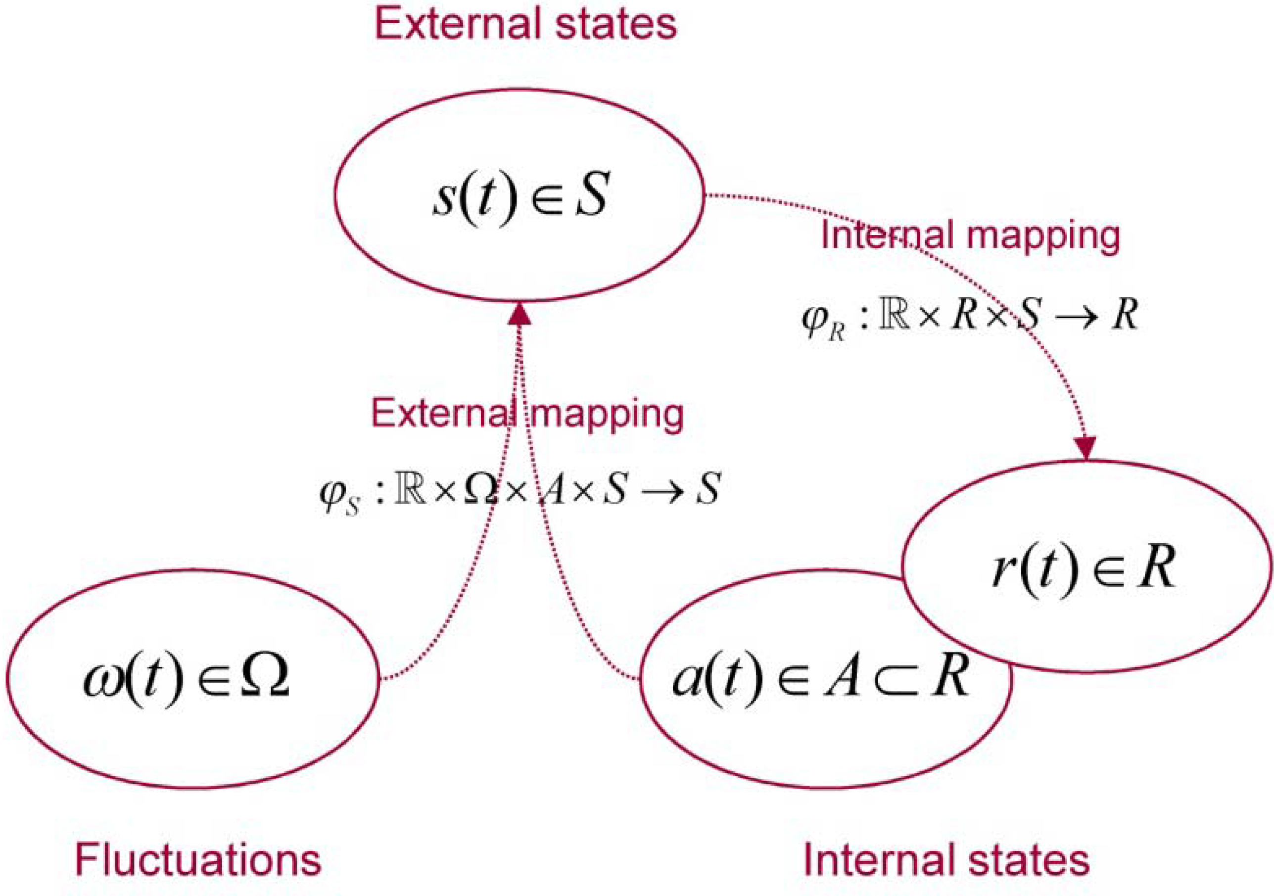
This section uses the formalism provided by random dynamical systems [34,35,36]. Roughly speaking, random dynamical systems combine a measure preserving dynamical system in the sense of ergodic theory, with a smooth dynamical system, generated by the solution to random differential equations. Random dynamical systems consist of a base flow and a dynamical system on some physical state space X d . The base flow ϑ : × Ω Ω comprises measure-preserving measurable functions ϑ t : Ω Ω for each time t . These functions constitute a group of transformations of a probability space ( Ω , , P ) , such that ( Ω , , P , ϑ ) is a measure preserving dynamical system. Here is a sigma algebra over Ω and P : [ 0 , 1 ] is a probability measure. The dynamical system ( R d , φ ) comprises a solution operator or flow map φ : × Ω × X X . This is a measurable function that maps to the (metric) state space X d and satisfies the cocycle property: φ ( τ , ϑ t ( ω ) ) φ ( t , ω ) = φ ( t + τ , ω ) . The flow map can be regarded as (being generated from) the solution x ( t ) : = φ ( t , ω ) ( x 0 ) to a stochastic differential equation of the form:
x ˙ ( t ) = f X ( x ) + g X ( x ) ω ( t ) x ( 0 ) = x 0
We use a Langevin form (as opposed to a differential form) for equation (1) because the fluctuations ω ( t ) : = ϑ t ( ω ) generated by the base flow can be continuous (differentiable). Here, we consider the base flow to represent universal or environmental dynamics and Ω to be a sample space. This sample space is the set of outcomes ω ( t ) Ω that result from the environment acting on the system. In other words, the environment is taken to be the measure preserving dynamical system ( Ω , , P , ϑ ) in which the dynamical system ( d , φ ) is immersed. The dynamical system is our biological system of interest and can be regarded as being generated from the solution to the differential Equation (1) describing its dynamical behaviour.
In what follows, we denote a particular system by the tuple m = ( d , φ ) . Equation (1) is particularly appropriate for biological systems, given that biological systems are normally cast as differential equations; from the microscopic level (e.g., Hodgkin Huxley equations) through macroscopic levels (e.g., compartmental kinetics in pharmacology) to population dynamics (e.g., Lotka-Volterra dynamics) [37]. In other words, the flow maps of random dynamical systems have the same form as existing models of biological systems that are cast in terms of differential equations pertaining to physical states. For example, the Hodgkin Huxley equations describe the dynamics of intracellular ion concentrations and transmembrane potentials, while Lotka-Volterra equations described changes in the ensemble distribution of physical states over large numbers of neurons or, indeed, conspecifics in evolution.
Crucially, we allow for a partition of the state space X = R × S , where R X is distinguished by the existence of a map φ R : × X R that precludes direct dependency on the base flow. In this sense, R X constitutes an internal state space, while S X constitutes an external state space. In this construction, the internal and external maps satisfy the following equalities:
φ R ( τ ) φ ( t , ω ) = φ R ( t + τ ) φ S ( τ , ϑ t ( ω ) ) φ ( t , ω ) = φ S ( t + τ , ω )
These maps can be regarded as the solutions to stochastic differential equations of the form:
s ˙ ( t ) = f S ( r , s ) + g S ( r , s ) ω ( t ) r ˙ ( t ) = f R ( r , s )
Finally, we allow for the possibility that the external map φ S : × Ω × A × S S may only depend on a subset of internal states A R . We will see later that these states allow the agent to act upon the environment. In this set up, internal states have dynamics that depend on external states and themselves, while external states depend on internal states and themselves but are also subject to fluctuations. See Figure 1 and Table 2. The distinction between external and internal states will become important below when considering self-organization in terms of constraints on, and only on, the dynamics of internal states.
Figure 1. This figure shows the statistical dependencies between fluctuations (assigned to the environment) and the states of a system (assigned to a biological agent). These dependencies are shown in terms of a probabilistic graphical model, where the arrows or edges denote conditional dependence. These dependencies are mediated by a (stochastic) external map and a (deterministic) internal map that constitute the dynamical system.
Entropy 14 02100 g001
Table 2. Summary of the random dynamical system formulation.
VariableDescription
X = R × S R d Physical state space a random dynamical system
ϑ : × Ω Ω Base flow of a random dynamical system
φ : × Ω × X X Flow or mapping to physical states
ω ( t ) : = ϑ t ( ω ) Ω Fluctuations generated by the base flow
R X Internal state space
S X External state space
A R Active states
φ S : × Ω × A × S S Mapping to external states
φ R : × R × S R Mapping to internal states

2.2. Ergodic Behaviour and Random Dynamical Attractors

To provide some intuition about the sorts of systems that might be modelled in this way, consider two special cases, open and closed systems: open systems have no internal states and X = S d . In this case, all states are subject to environmental fluctuations and the flow map corresponds to the solution to stochastic differential equations―as in equation (1). Examples here might include models in computational biology that are used to study self-organizing systems that attain non-equilibrium steady-state [29,38,39,40] or persistence in fluctuating environments [41]. The key aspect of these systems is that they possess a characteristic distribution of physical states―usually referred to as steady-state and yet operate far from equilibrium. Key examples here range from intracellular kinetics in molecular biology through to neuronal circuits in neuroscience and, at the highest level, the self organisation of entire phenotypes, as studied in theoretical biology and situated (embodied) cognition.
Closed systems have no external states and X = R d such that random fluctuations can be discounted. The corresponding flow map then becomes a deterministic mapping among internal states and can be associated with the solution to ordinary differential equations with deterministic attractors (in the classical or Milnor sense). Examples of these systems could be classical attractors [42] and coupled networks that exhibit complicated and itinerant behaviour, with weakly attracting sets [43,44,37,45]. Here, we consider systems with both external and internal states that furnish models of a system in a changing (and possibly non-ergodic) environment.

2.3. Circular Causality and Active Systems

In synergetics and the study of self-organizing systems [46,47], one could associate the external states with microscopic system variables (stable modes) that show fast fluctuations, while the internal states might correspond to the macroscopic order parameters (unstable modes) that enslave them. The same theme of circular causality is seen in nonlinear Fokker-Planck formulations of coupled nonlinear random dynamical systems [48,49], where (macroscopic) mean field effects couple back to the density over (microscopic) states by changing their flow. This is a ubiquitous sort of behaviour that arises when some states “see” a large number of other states, such that their flow is determined, effectively, by the average over the states they see. This means the microscopic dynamics are caused by macroscopic mean field effects that are constituted (caused by) microscopic states.
The sorts of systems we have in mind here are biological systems, where one can regard the (microscopic) external states s ( t ) = φ S ( t , ω ) ( x 0 ) as the state of sensory receptors, while the internal states r ( t ) = φ R ( t ) ( x 0 ) that include a ( t ) A R , respond to sensory perturbations. For example, in a single cell, external states could be associated with the states of transmembrane receptors, while the internal states might include the concentrations of intracellular metabolites, depolarization or temperature [50,51]. Later, we will consider the brain, were external states could correspond to sensory input and internal states to macroscopic variables, like neuronal firing rates. We will refer to a ( t ) A as active states because they control how environmental fluctuations are sampled by the sensory states. Active states could correspond to the states of the system that change its physical configuration or exposure to outcomes (e.g., the motion of flagella in single cell organisms or sensory epithelia like the retina). In summary, the opportunity for circular causality arises because internal states depend on external states, while the internal couple back to the external states by changing their flow or motion: see equation (3).
We are interested in systems whose physical states x ( t ) = φ ( t , ω ) ( x 0 ) are confined to a bounded subset of states and remain there indefinitely. In terms of random dynamical systems, this means the system possesses a random dynamical attractor [34,35,52], which we assume is ergodic. This is a random compact set A ( ω ) X that is invariant under the flow map such that φ ( t , ω ) ( A ( ω ) ) = A ( ϑ t ( ω ) ) . In terms of ergodic theory [53], this means there is a unique and stationary ergodic density p ( x | m ) that is proportional to the amount of time each state is occupied. Alternatively, the recurrence time between visits to states in the attracting set is inversely proportional to the ergodic density. This ergodic density is central to the arguments in this paper. It characterises the distribution of states occupied by a system over the long term and is therefore subject to important constraints, given that the system persists over long periods of time. Later, we will see that marginal ergodic density over external states can be interpreted in a statistical or information theoretic sense as the marginal likelihood or evidence for a model of external dynamics entailed by the system. This allows us to interpret the internal dynamics of the system as an abstract form of inference and information exchange with the environment.
The ergodic density can be characterized by its Shannon entropy, to which the long-term average of self-information or surprisal ( x ( t ) ) converges, almost surely:
p ( x | m ) = lim T 1 T 0 T δ ( x x ( t ) ) d t      a . s . , ( X | m ) = X p ( x | m ) ln p ( x | m ) d x = lim T 1 T 0 T d t ( x ( t ) )      a . s . , ( x ( t ) ) = ln p ( x ( t ) | m ) B p ( x ( t ) | m ) d x = P ( { ω Ω : φ ( t , ω ) ( x 0 ) B } )
The ergodic density p ( x | m ) is an invariant probability measure that can be regarded as the probability of finding the system in any state when observed at a random point in time. The existence of the ergodic density and its underlying attractor ensures the system has invariant characteristics that underwrite its existence over time. Strictly speaking, the entropy in (4) is a differential entropy (as opposed to a normal or absolute entropy), because we are dealing with continuous states.
Remarks:
The integral in the final equality above is over the Lebesgue measure λ ( B ) of any measurable subset B X of the (metric) state space and defines the ergodic density in terms of the system’s flow. The slightly unusual conditioning of probability densities on the system m = ( R d , φ ) . simply associates the probability densities with a particular system. This notation comes from Bayesian statistics, where one can consider different systems (with different internal states) that might possess the same external states. We will exploit this perspective later, under which m = ( R d , φ ) can be regarded as a model of environmental fluctuations and internal states, r ( t ) = φ R ( t ) ( x 0 ) as representations of their causes. Finally, note that the Shannon entropy above is an information entropy as opposed to a metric or Kolmogorov Sinai entropy. In other words, it is an invariant measure that summarizes the number of distinct states the system occupies. This can be expressed more formally in terms of the entropy of the ergodic density:
Lemma 1
(ergodic entropy): the entropy of the ergodic density of a random dynamical system m = ( d , φ ) is upper bounded by the Lebesgue measure of its attractor (if it exists):
H ( X | m ) ln λ ( A ( ω ) )
Proof:
The entropy is maximal when the ergodic density is distributed uniformly over the attracting set A ( ω ) X [54]. In this case:
p ( x | m ) = { 1 / λ ( A ( ω ) ) x A ( ω ) 0 x A ( ω )           H ( X | m ) = ln λ ( A ( ω ) )
where the first equality ensures that the integral of the ergodic density over states is unity.
In brief, the measure or volume of a system’s attracting set places an upper bound on the entropy of its ergodic density. In other words, if the measure is small then the entropy must be small[er]. We now use this to motivate a definition of ergodic random dynamical systems that actively maintain low entropy. These systems occupy a limited repertoire of attracting states and will thereby exhibit a homoeostasis [25]. We associate this sort of system with biological systems, like single cells and more complex organisms.
Definition 1
(active systems): an ergodic random dynamical system m = ( d , φ ) is said to be active if it possesses an internal map that satisfies (locally) the extremal condition:
φ R = arg min φ R H ( S | m ) H ( S | m ) = p ( s | m ) ln p ( s | m ) = lim T 1 T 0 T d t ( s ( t ) )     a.s. , ( s ( t ) ) = ln p ( s ( t ) | m ) B p ( s ( t ) | m ) d x = P ( { ω Ω : φ S ( t , ω ) ( x 0 ) B } )
In other words, the internal states r ( t ) = φ R ( t ) ( x 0 ) minimize the entropy of the ergodic density over external states. The minimization of the entropy with respect to internal states generated by the deterministic map φ R : × X R will depend upon the probabilistic map from the environment φ S : × Ω × X S . Put simply, the internal states of active systems minimise the dispersion of their external or sensory states.
The motivation for Definition 1 is simple: systems that do not minimize their entropy are unlikely to exist, in the sense that the measure of their random dynamical attractors A ( ω ) can be arbitrarily large and their recurrence times arbitrarily long. In this view, (active) random dynamical systems that exist are simply solutions to (7), under the constraints provided by environmental fluctuations. Crucially, active systems minimize surprisal and conform to the principle of least action:
Lemma 2
(principle of least action): the internal states of an active system minimize the Lagrangian or surprisal ( s ( t ) ) such that the variation δ r S of action S with respect to its internal states r ( t ) R vanishes:
r ( t ) = φ R ( t ) ( x 0 ) = arg min r ( s ( t ) ) r ( s ( t ) ) = 0 δ r S = 0 S = 0 T d t ( s ( t ) )
Here, action S is the time or path-integral of the Lagrangian ( s ( t ) ) , which is the surprisal (or more simply surprise) associated with external states. Equation (8) also implies the converse; if the variation of action with respect to internal states is zero, then the system is active (from Definition 1)
Proof:
The proof is straightforward and rests on noting that action and the entropy of the ergodic density over external states are related via the ergodic theorem [53]. From (7):
T ( S | m ) = 0 T d t ( s ( t ) ) = S     a.s. ,
where T + is a suitably long observation time. This equivalence means that δ r S = 0 δ r ( S | m ) = 0 φ R = arg min φ R H ( S | m ) , where r ( s ( t ) ) = 0 δ r S = 0 by the fundamental Lemma of variational calculus.
Remark (evidence maximization):
Because the Lagrangian or surprise ( s ( t ) ) = ln p ( s ( t ) | m ) is the negative log-evidence in Bayesian statistics, active systems maximize the long term time-average of their log-evidence (by Definition 1). Heuristically, this means that they actively sample their environment to maximize the evidence for their own existence [2]. We will now look more closely at this heuristic from the point of view of active (Bayesian) inference and the free energy principle:

3. Active Inference and the Free Energy Principle

The notion of random dynamical systems m = ( d , φ ) that possess internal states allows one to cast self-organization in terms of a deterministic map φ R : × X R (Definition 1), with minimal assumptions about how the system is coupled to the environment through φ S : × Ω × X S , or the dynamics of the environment ( Ω , , P , ϑ ) . In this setting, self-organization can be understood in terms of a circular causality, in which internal (e.g., macroscopic) states entrain the external (e.g., microscopic) states from which they are derived. The outstanding issue is how the deterministic internal map minimizes the surprise or entropy of external states, given that internal states do not ‘know’ how they affect external states. Intuitively, the solution considered below regards the system as optimizing a probabilistic (generative) model of external dynamics, which is used to minimize surprise. More formally, we want to express the internal states in terms of some real valued and measurable functional : × X of states that satisfies (7). To see how this can be done we need to define three further quantities:
Definition 2
(the generative model): Let the density p ( s ( t ) | m ) defined in equation (7) be expressed in terms of some arbitrary parameters ψ ( t ) Ψ that are themselves (fictive) random variables:
p ( s ( t ) | m ) = Ψ p ( s ( t ) , ψ ( t ) | m ) d ψ p ( s ( t ) , ψ ( t ) | m ) = p ( s ( t ) | ψ ( t ) , m ) p ( ψ ( t ) | m )
The generative model is then defined by the probability density function p ( s ( t ) , ψ ( t ) | m ) . In statistics p ( s ( t ) | ψ ( t ) , m ) is known as the likelihood and p ( ψ ( t ) | m ) is called a prior. As noted above, p ( s ( t ) | m ) is known as the marginal likelihood or evidence.
Definition 3
(the proposal density): Let q ( ψ ( t ) | μ ( t ) ) denote a mapping q : R × Ψ × R R such that for all ψ ( t ) Ψ :
q ( ψ ( t ) | μ ( t ) ) 0 Ψ q ( ψ ( t ) | μ ( t ) ) d ψ = 1
This means that q ( ψ ( t ) | μ ( t ) ) plays the role of an arbitrary probability density function over the parameters of the generative model, where this density is parameterized by μ ( t ) R . Crucially, μ ( t ) r ( t ) are internal states, such that the internal state of the system induces a proposal density over the variables that parameterise the evidence or marginal likelihood of external states.
Remark:
The (fictive) variables ψ ( t ) Ψ are not observable quantities; they are induced with the proposal density and only exist to parameterise the marginal likelihood. We will see later that they can be regarded as the (fictive) causes of environmental fluctuations, under a generative model. In statistics and machine learning they are often called hidden states, because they are not observable.
Definition 4
(free energy): the free energy is now defined in terms of the proposal and generative densities as the following expectation [9,12,6]:
( x ( t ) ) = Ψ q ( ψ ( t ) | μ ( t ) ) ln q ( ψ ( t ) | μ ( t ) ) p ( s ( t ) , ψ ( t ) | m ) d ψ
Note that the free energy is a scalar function of, and only of, the system states : × R × S .
With these definitions in place, we can now express the internal dynamics of active systems in terms of a free energy principle:
Proposition 1
(the free energy principle): Let m = ( d , φ ) be an ergodic random dynamical system with state space X = R × S d . If the internal states r ( t ) R minimize free energy, then the system conforms to the principle of least action and is an active system (by Lemma 2):
r ( t ) = φ R ( t ) ( x 0 ) = arg min r ( x ( t ) ) δ r S = 0
Proof:
From Definition 3, we can express free energy in terms of surprise and a Kullback-Leibler divergence or cross entropy:
( x ( t ) ) = ( s ( t ) ) + Ψ q ( ψ ( t ) | μ ( t ) ) ln q ( ψ ( t ) | μ ( t ) ) p ( ψ ( t ) | s ( t ) , m ) d ψ = ( s ( t ) ) + D K L [ q ( ψ ( t ) | μ ( t ) ) | | p ( ψ ( t ) | s ( t ) , m ) ]
By Gibbs inequality D K L 0 [55]. This means that when free energy is minimized with respect to μ ( t ) R the divergence will be zero (provided such a solution exists – please see below). This means free energy becomes surprise ( x ( t ) ) = ( s ( t ) ) and its variation with respect to a ( t ) R vanishes:
a ( t ) = arg min a ( x ( t ) ) a ( x ( t ) ) = 0 a ( s ( t ) ) = 0 δ a S = 0
From (8) we see that surprise does not depend on μ ( t ) , which means μ ( t ) = 0 δ μ S = 0 and therefore δ r S = 0 from (15).
Remarks:
these are standard results that underlie variational Bayesian methods such as variational Bayes and Bayesian filtering [9,11,12]. In short, minimizing free energy with respect to the internal states renders it the surprise that is minimized by active states. This implicitly minimizes the path integral of surprise over time (action). In the above proof, we have assumed that – when minimised – the divergence term is zero. This rests on the assumption that the proposal density can have the same form as the conditional density in the denominator of the divergence term. As we will see below, this corresponds to exact Bayesian inference. More generally, when the form of the proposal density does not permit an exact match to the conditional density, the free energy becomes a bound approximation to surprise and we have what is known as approximate Bayesian inference [9]. To conclude this section, we consider three important corollaries of the free energy principle, starting with the Bayesian interpretation:
Corollary 1
(Bayesian inference): Systems that conform to the free energy principle represent the causes of their sensory states in a Bayesian sense: This follows from (14), where minimizing free energy with respect to the internal states minimizes the divergence between the proposal density and the posterior density over the parameters of the likelihood function:
μ ( t ) = arg min μ ( x ( t ) ) = arg min μ D K L ( q ( ψ ( t ) | μ ( t ) ) | | p ( ψ ( t ) | s ( t ) , m ) )
In other words, the optimal proposal density q ( ψ ( t ) | μ ( t ) ) – parameterized by internal states – becomes the posterior p ( ψ ( t ) | s ( t ) , m ) , under the model entailed (see below) by the system. In a neurobiological setting, this is known as the Bayesian brain hypothesis [7,8] and appeals to the notion that the brain makes inferences about the causes of its sensory inputs [4,6]: see [2] for a review. In this setting, the parameters of the likelihood function can be regarded as hidden states in the environment or hidden causes of sensory states, while the internal states become representations; in the sense that they parameterize the posterior density over (fictive) causes. Generally, because one cannot guarantee the disappearance of the divergence in Equation 14, the ensuing inference is referred to as approximate Bayesian inference. This form of inference underlies the majority of variational Bayesian procedures.
Corollary 2
(active inference): Systems that conform to the free energy principle will selectively sample what they ‘expect to see’. This follows from a final rearrangement of free energy in terms of complexity and accuracy or the log likelihood of sensory states under the proposal density:
( x ( t ) ) = Ψ q ( ψ ( t ) | μ ( t ) ) ( s ( t ) ) d ψ + Ψ q ( ψ ( t ) | μ ( t ) ) ln q ( ψ ( t ) | μ ( t ) ) p ( ψ ( t ) | s ( t ) , m ) d ψ = Ψ q ( ψ ( t ) | μ ( t ) ) ln q ( ψ ( t ) | μ ( t ) ) p ( ψ ( t ) | s ( t ) , m ) p ( s ( t ) | m ) d ψ = D K L ( q ( ψ ( t ) | μ ( t ) ) | | p ( ψ ( t ) | m ) ) Ψ q ( ψ ( t ) | μ ( t ) ) ln p ( s ( t ) | ψ ( t ) , m ) d ψ a ( t ) = arg min a ( x ( t ) ) = arg max a Ψ q ( ψ ( t ) | μ ( t ) ) ln p ( s ( t ) | ψ ( t ) , m ) d ψ
This is called active inference and manifests as a selective sampling of (typical) sensory states that are most likely under the system’s posterior beliefs (by Corollary 1). It should be noted that we have not been explicit about how sensory states depend upon active states. In a practical setting, (17) is usually implemented using a generalized gradient descent (see next section), where the generalized motion of sensory states is controlled by active states. Active inference in biological systems has been introduced as a way of understanding motor control and behaviour in neuroscience. In this setting, the minimisation of free energy with respect to action reduces to simple reflexes. See Table 1 and [21].
Corollary 3
(Maximum entropy principle): From the representational perspective of corollary 1, minimizing variational free energy entails maximizing the entropy of the proposal density. This can be seen easily by rewriting the expression for free energy in terms of the negative entropy of the proposal density and an expected log density:
( x ( t ) ) = H [ q ( ψ ( t ) ) ] Ψ q ( ψ ( t ) | μ ( t ) ) ln p ( s ( t ) , ψ ( t ) | m ) d ψ H [ q ( ψ ( t ) ) ] = Ψ q ( ψ ( t ) | μ ( t ) ) ln q ( ψ ( t ) | μ ( t ) ) d ψ
This means that the proposal density encoding a probabilistic representation of hidden states should conform to the maximum entropy principle [32] (under the constraint that it provides a plausible explanation for sensory states), which can be regarded as a generalization of Laplace’s principle of indifference. Heuristically, this ensures generic explanations for external or sensory states that do not depend on overly specific (low entropy) beliefs about how they were caused (cf., Occam's razor).
Corollary 4
(entailment): A system can be said to entail a generative model when a pair of probability density functions p ( s ( t ) , ψ ( t ) | m ) and q ( ψ ( t ) | μ ( t ) ) satisfy (13). The existence of the proposal density q ( ψ ( t ) | μ ( t ) ) is central to this entailment and means that the internal states ‘represent’ the parameters of the generative model in a probabilistic sense.
Entailment is important because it means the internal states of a system encode or transcribe causal regularities in the processes generating external states. This means that the system behaves as if it is a model of the environment. This means that much can be inferred about the system’s environment from the dynamics of its internal states; provided one can identify or approximate the proposal and generative densities that satisfy (13). In one sense, identifying these densities is the key to understanding the nature of the system and how it has adapted to its environment. This is probably best illustrated when applying the free energy principle to the brain to understand its functional architecture [56] and the nature of neuronal codes [57]. In the final section, we will look at message passing in the brain under the free energy principle to illustrate how the theoretical approach above has been applied in practice. First, we examine systems that minimise free energy in terms of information theoretic descriptions.

4. Perception, Free Energy and the Information Bottleneck

In the next two sections, we will focus on perception from the point of view of information theory and biological implementation in the brain, respectively. This section considers free energy minimisation in light of the information bottleneck method [58] to show that they are internally consistent – therefore suggesting that the information bottleneck approach may be a useful way to describe biological self-organisation.

4.1. The Information Bottleneck

In its broadest (and simplest) sense, the information bottleneck method seeks to optimise the trade-off between accuracy and complexity when summarising hidden states, given a joint probability distribution over hidden states and observations (the generative model in Definition 2). This trade-off provides an important constraint on inferring hidden states and – in Bayesian terms – inference. Given that both the information bottleneck method and the free energy formulation are information theoretic formulations one might anticipate that they lead to the same sorts of optimal inference. Indeed, (17) shows that minimising free energy corresponds to minimising complexity, while maximising accuracy. The corresponding trade-off in the information bottleneck method can be expressed in terms of a criterion:
S B = I ( R ; Ψ ) I ( S ; R )
Here I ( R ; Ψ ) and I ( S ; R ) correspond to the mutual information between internal states and hidden states and between sensory (external) states and internal states, respectively. Minimising the first term, corresponds to minimising complexity, while minimising the second maximises the accuracy of the representation of sensory states by internal states. In the present context, we can express the information bottleneck criterion in terms of its constituent entropies:
S B = H ( R | m ) H ( R | Ψ , m ) H ( S | m ) + H ( S | R , m ) S B * = H ( R | m ) + H ( S | R , m )
The entropies in (20) have been conditioned on m to emphasise that the underlying probability distributions are defined in relation to a generative model. The quantity S B * is a reduced information bottleneck criterion that follows from the fact that, from the point of view of inference, the entropy of sensory states is fixed and can be eliminated from the criterion. Similarly, the conditional entropy (equivocation) of the internal states, given the hidden states can be eliminated, because the hidden states are unknown. In this reduced form, the information bottleneck requires the internal states (representations) to predict sensory states accurately, under the constraint that their entropy is small. In other words, there are a small number of internal states with minimal dispersion that ensure complexity is minimised. So can the (reduced) information bottleneck criterion be derived from free energy minimisation?

4.2. Free Energy Minimisation and the Information Bottleneck

If we assume (for simplicity) that the proposal density is a point of mass (delta function) over a particular value of hidden states μ ( t ) R , then the ensuing (reduced) free energy can be expressed as (from equation 17):
* ( t ) = ln p ( μ ( t ) | m ) ln p ( s ( t ) | μ ( t ) , m )
From point of view of Bayesian inference, this corresponds to maximum a posteriori point estimation and returns the most likely value of hidden states. If we now consider minimising the path integral of this (reduced) free energy, under ergodic assumptions we obtain:
S F * = d t * ( t ) = H ( R | m ) + H ( S | R , m )
This path integral is exactly the same as the (reduced) information bottleneck criterion, demonstrating a pleasing consilience between the free energy formulation and the information bottleneck approach. This formal equivalence rests upon the ergodic reduction of variational free energy through maximum a posteriori Bayesian inference. Heuristically, is illustrates that the complexity minimisation, implicit in the information bottleneck method, appeals to the prior beliefs entailed by the system; which reduce the dispersion of internal states summarising hidden states. In summary, this section suggests that active systems that minimise variational free energy – through optimising their internal states – comply with the constraints afforded by the information bottleneck method. The next section we consider how real biological systems might implement this minimisation. The following section is a brief summary of the material presented in [2].

5. Perception in the Brain

This section focuses on the implication of the theoretical arguments above– that active systems perform some form of approximate Bayesian inference. This is probably best exemplified in sensory neuroscience; where the notion of the Bayesian brain has a long history [4]. The minimization of free energy with respect to a system’s internal states (16) is particularly revealing when applied to the brain. The key to link this minimization with the dynamics of biological systems rests on assuming their internal states perform a gradient descent on free energy. A general scheme that performs this gradient descent is generalized filtering [59]:
μ ˜ ˙ = D μ ˜ μ ˜ ( s ˜ , μ ˜ )
This has the same form as Bayesian (e.g., Kalman-Bucy) filtering, used in time series analysis. In this setting, the internal states μ ˜ ( t ) R correspond to conditional expectations or maximum a posteriori estimates of hidden states ψ ( t ) Ψ . In neurobiological formulations, these are associated with neuronal activity. The ~ notation denotes variables in generalized coordinates of motion; for example, s ˜ = [ s , s , s , ] T . The first term in (19) is a prediction based upon a matrix differential operator D that returns the generalized motion of the expectation, such that D μ ˜ = [ μ , μ , μ , ] T . The second term is usually expressed as a mixture of prediction errors (see below) that ensures the changes in conditional expectations are Bayes-optimal predictions about hidden states ‘causing’ fluctuations in the world. Heuristically, one can regard (19) as a gradient descent in a moving frame of reference, such that when free energy is minimized, the motion of the mean becomes the mean of the mean of the motion μ ˜ ˙ = D μ ˜ . See [59] for details.
Solutions of (23) correspond to Bayes-optimal neuronal dynamics that encode the predictions of hidden states. These predictions depend upon the brain’s model of the world, which is usually assumed to have the following (hierarchical) form:
s ( t ) = f ( 1 , v ) ( u ( 1 ) , v ( 1 ) ) + ω ( 1 , v ) u ˙ ( 1 ) = f ( 1 , u ) ( u ( 1 ) , v ( 1 ) ) + ω ( 1 , u ) v ( i 1 ) = f ( i , v ) ( u ( i ) , v ( i ) ) + ω ( i , v ) u ˙ ( i ) = f ( i , u ) ( u ( i ) , v ( i ) ) + ω ( i , u )
Here, ( f ( i , u ) , f ( i , v ) ) are nonlinear functions of hidden states and causes ψ ( t ) ( u , v ) that generate sensory inputs s ( t ) at the first (lowest) level. Random fluctuations ( ω ( i , u ) , ω ( i , v ) ) on the motion of hidden states and causes are conditionally independent and enter each level of the hierarchy. They model sensory noise at the first level and induce uncertainty about states at higher levels. Hidden causes v ( t ) = ( v ( 1 ) , v ( 2 ) , . ) link levels, whereas hidden states u ( t ) = ( u ( 1 ) , u ( 2 ) , . ) link dynamics over time. Hidden states and causes are abstract quantities (like the motion of an object in the field of view) that the brain uses to explain or predict sensations. In this hierarchical form, the output of one level acts as an input to the next to produce complicated models with deep (hierarchical) structure. Gaussian assumptions about the random fluctuations in (23) provide the generative model in Definition 2: p ( s ( t ) , ψ ( t ) | m ) , where their amplitude is encoded by their precisions ( Π ˜ ( i , u ) , Π ˜ ( i , v ) ) .

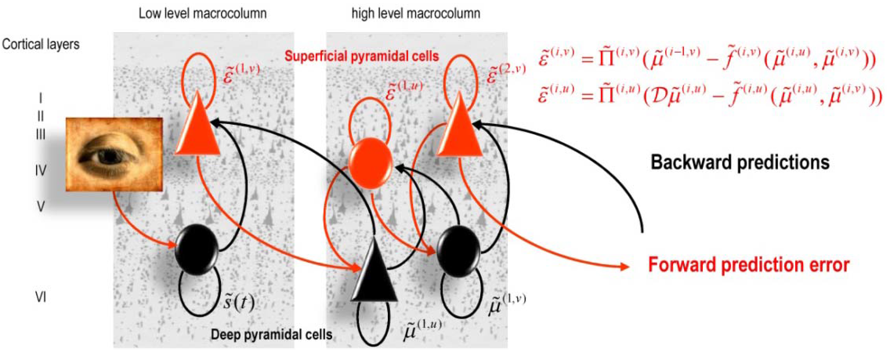
5.1. Predictive Coding and Free Energy Minimization

Given the form of the generative model (24), one can now write down the differential equations (25) describing neuronal dynamics in terms of (precision-weighted) prediction errors ( ε ˜ ( i , u ) , ε ˜ ( i , v ) ) that represent the difference between conditional expectations about hidden states and causes ( μ ˜ ( i , u ) , μ ˜ ( i , v ) ) and their hierarchical predictions (using A B : = A T B ):
μ ˜ ˙ ( i , v ) = D μ ˜ ( i , v ) + f ˜ ( i , v ) μ ˜ ( i , v ) ε ˜ ( i , v ) + f ˜ ( i , u ) μ ˜ ( i , v ) ε ˜ ( i , u ) ε ˜ ( i + 1 , v ) μ ˜ ˙ ( i , u ) = D μ ˜ ( i , u ) + f ˜ ( i , v ) μ ˜ ( i , u ) ε ˜ ( i , v ) + f ˜ ( i , x ) μ ˜ ( i , u ) ε ˜ ( i , u ) D ε ˜ ( i , u ) ε ˜ ( i , v ) = Π ˜ ( i , v ) ( μ ˜ ( i 1 , v ) f ˜ ( i , v ) ) ε ˜ ( i , u ) = Π ˜ ( i , u ) ( D μ ˜ ( i , u ) f ˜ ( i , u ) )
This particular form of generalized filtering is called generalized predictive coding and rests on assuming a Gaussian form for the proposal density in Definition 3: q ( ψ | μ ˜ ) = N ( μ ˜ , Σ ( μ ˜ ) ) . This is known as the Laplace assumption; see [14] for an introduction to predictive coding in visual neuroscience and [13] for an introduction to the Laplace assumption in the setting of variational free energy minimization.
It is difficult to overstate the generality and importance of (25): its solutions grandfather nearly every known statistical estimation scheme, under parametric assumptions about additive noise. These range from ordinary least squares to advanced variational deconvolution schemes. In neural network terms, (25) says that error-units receive predictions from the same level and the level above. Conversely, prediction-units are driven by prediction errors from the same level and the level below. These constitute bottom-up and lateral messages that drive conditional expectations towards a better prediction to reduce the prediction error in the level below. This is the essence of recurrent message passing between hierarchical levels in the brain that suppress free energy or prediction error. See [18] for a more detailed discussion. In neurobiological implementations of this scheme, the sources of bottom-up prediction errors, in the cortex, are thought to be superficial pyramidal cells that send forward connections to higher cortical areas. Conversely, predictions are conveyed from deep pyramidal cells, by backward connections, to target (polysynaptically) the superficial pyramidal cells encoding prediction error [60]. See Figure 2. A detailed consideration of the form of (25) leads to several predictions about the brain circuits subtending perception; many of which are remarkably consistent with empirical observations. A few examples are provided in Table 3.
Table 3. Structural and functional aspects of the brain that can be explained by free energy minimization: see [33] for details.
DomainPredictions
Anatomy:
Explains the hierarchical deployment of cortical areas, recurrent architectures with functionally asymmetric forward and backward connections
Hierarchical cortical organization
Distinct neuronal subpopulations, encoding expected states of the world and prediction error
Extrinsic forward connections convey prediction error (from superficial pyramidal cells) and backward connections mediate predictions (from deep pyramidal cells)
Functional asymmetries in forwards (linear) and backwards (nonlinear) connections are mandated by nonlinearities in the generative model encoded by backward connections
Principal cells elaborating predictions (e.g., deep pyramidal cells) show distinct (low-pass) dynamics, relative to those encoding error (e.g., superficial pyramidal cells)
Recurrent dynamics are intrinsically stable because they suppress prediction error (i.e., no strong loops)
Physiology:
Explains both (short-term) neuromodulatory gain-control and the nature of evoked responses
Scaling of prediction errors, in proportion to their precision, affords the cortical bias or gain control seen in attention
Neuromodulatory factors may play a dual role in modulating postsynaptic responsiveness (e.g., through after-hyperpolarizing currents) and synaptic plasticity
Sensory responses are greater for surprising, unpredictable or incoherent stimuli
The attenuation of responses encoding prediction error, with perceptual learning, explains repetition suppression (e.g., mismatch negativity in electroencephalography)
Although we have cast generalized Bayesian filtering in terms of neuronal message passing, the generality of the principles established in the previous sections suggests that the same formalism might be applied to any biological system that exhibits dynamics. Indeed, there are current attempts to apply exactly the same analysis above to the intracellular kinetics of single cells [51]. In this context, the internal states are not neuronal firing rates but are transmembrane depolarization or the intracellular concentrations of various ionic or molecular substrates. Whether the same sort of analysis could be applied to the dynamical systems seen in evolutionary theory and behavioural economics remains to be seen but is an intriguing possibility: see e.g. [61].
Figure 2. This figure provides a schematic overview of the message passing scheme implied by Equation 21. In this scheme, neurons are divided into prediction (black) and prediction error (red) units that pass messages to each other, within and between hierarchical levels (macrocolumns). Superficial pyramidal cells (red) send forward prediction errors to deep pyramidal cells (black), which reciprocate with predictions that are conveyed by (polysynaptic) backward connections. This process continues until the amplitude of prediction error has been minimized and the predictions are optimized in a Bayesian sense. The prediction errors are the (precision-weighted) difference between conditional expectations encoded at any level and top-down or lateral predictions. The Roman numerals designate the cortical layers in which neurons are situated.
Entropy 14 02100 g002

6. Conclusions

This paper describes a general, if somewhat abstract, motivation for a variational free energy principle that has a wide explanatory scope in neurobiology and has construct validity in relation to important information theoretic treatments, in particular, the information bottleneck method [58]. We have tried to show that free energy minimization may be an imperative for all self-organizing biological systems and speculate that the attending biological insights may generalize beyond the neurosciences. The implication is that any biological system, from a single-cell organism to a social structure should have, encoded in its internal (macroscopic) states, a representation of causal structure in its external milieu; and should act to fulfil predictions based on that representation. Put simply, biological systems entail a model of their environment and act to maximize the evidence for that model and, implicitly, their own existence.
We conclude by noting that active systems do not purposefully construct the models that they entail, in the sense that if they did not entail a model that satisfies (13) they would not exist; or only exist for short periods of time (until their external states were dispersed by environmental fluctuations). In other words, Equation (13) simply provides dynamics that enable systems to persist in the face of fluctuating environmental influences. In summary, the free energy principle is just a delicate reconstruction of the principle of least action, in the setting of random dynamical systems. Credit for the principle of least action is commonly given to Pierre Louis Maupertuis [62,63], who wrote: “The laws of movement and of rest deduced from this principle being precisely the same as those observed in nature, we can admire the application of it to all phenomena. The movement of animals, the vegetative growth of plants... are only its consequences; and the spectacle of the universe becomes so much the grander, so much more beautiful, the worthier of its Author, when one knows that a small number of laws, most wisely established, suffice for all movements.”

Acknowledgements

This work was funded by the Wellcome Trust. We would like to thank Simon McGregor for encouraging this formulation and Sebastian Schreiber for critical comments on an earlier version of this paper.

References

  1. Bialek, W.; Nemenman, I.; Tishby, N. Predictability, complexity, and learning. Neural Computat. 2001, 13, 2409–2463. [Google Scholar] [CrossRef] [PubMed]
  2. Friston, K. The free-energy principle: a unified brain theory? Nat. Rev. Neurosci. 2010, 11, 127–138. [Google Scholar] [CrossRef] [PubMed]
  3. Friston, K. A theory of cortical responses. Philos. Trans. R. Soc. Lond B Biol. Sci. 2005, 360, 815–836. [Google Scholar] [CrossRef] [PubMed]
  4. Helmholtz, H. Concerning the perceptions in general. In Treatise on Physiological Optics, 3rd ed.; Dover Publications: New York, NY, USA, 1962. [Google Scholar]
  5. Gregory, R.L. Perceptual illusions and brain models. Proc. R. Soc. Lond. B 1968, 171, 179–196. [Google Scholar] [CrossRef]
  6. Dayan, P.; Hinton, G.E.; Neal, R. The Helmholtz machine. Neural Comput. 1995, 7, 889–904. [Google Scholar] [CrossRef]
  7. Knill, D.C.; Pouget, A. The Bayesian brain: the role of uncertainty in neural coding and computation. Trends Neurosci. 2004, 27, 712–719. [Google Scholar] [CrossRef] [PubMed]
  8. Yuille, A.; Kersten, D. Vision as Bayesian inference: analysis by synthesis? Trends Cogn. Sci. 2006, 10, 301–308. [Google Scholar] [CrossRef] [PubMed]
  9. Beal, M.J. Variational Algorithms for Approximate Bayesian Inference. Ph.D. Thesis, University College London, London, UK, 2003. [Google Scholar]
  10. Feynman, R.P. Statistical Mechanics; Reading MA: Benjamin, TX, USA, 1972. [Google Scholar]
  11. Hinton, G.E.; van Camp, D. Keeping neural networks simple by minimizing the description length of weights. In Proceedings of the Sixth Annual Conference on Computational Learning Theory, Santa Cruz, NY, USA, July 1993; pp. 5–13.
  12. MacKay, D.J. Free-energy minimisation algorithm for decoding and cryptoanalysis. Electron. Lett. 1995, 31, 445–447. [Google Scholar] [CrossRef]
  13. Friston, K.; Mattout, J.; Trujillo-Barreto, N.; Ashburner, J.; Penny, W. Variational free energy and the Laplace approximation. Neuroimage 2007, 34, 220–234. [Google Scholar] [CrossRef] [PubMed]
  14. Rao, R.P.; Ballard, D.H. Predictive coding in the visual cortex: a functional interpretation of some extra-classical receptive-field effects. Nat. Neurosci. 1999, 2, 79–87. [Google Scholar] [CrossRef] [PubMed]
  15. Ortega, P.A.; Braun, D.A. A Minimum Relative Entropy Principle for Learning and Acting. J. Artif. Intell. Res. 2010, 38, 475–511. [Google Scholar]
  16. Friston, K.; Kilner, J.; Harrison, L. A free energy principle for the brain. J. Physiol. Paris. 2006, 100, 70–87. [Google Scholar] [CrossRef] [PubMed]
  17. Ashby, W.R. Principles of the self-organizing dynamic system. J. Gen. Psychol. 1947, 37, 125–128. [Google Scholar] [CrossRef] [PubMed]
  18. Friston, K.; Kiebel, S. Cortical circuits for perceptual inference. Neural. Netw. 2009, 22, 1093–1104. [Google Scholar] [CrossRef] [PubMed]
  19. Kiebel, S.J.; Daunizeau, J.; Friston, K.J. Perception and hierarchical dynamics. Front. Neuroinform. 2009, 3, 20. [Google Scholar] [CrossRef] [PubMed] [Green Version]
  20. Feldman, H.; Friston, K.J. Attention, uncertainty, and free-energy. Front. Hum. Neurosci. 2010, 4, 215. [Google Scholar] [CrossRef] [PubMed]
  21. Friston, K.J.; Daunizeau, J.; Kilner, J.; Kiebel, S.J. Action and behavior: a free-energy formulation. Biol. Cybern. 2010, 102, 227–260. [Google Scholar] [CrossRef] [PubMed]
  22. Friston, K.; Mattout, J.; Kilner, J. Action understanding and active inference. Biol. Cybern. 2011, 104, 137–160. [Google Scholar] [CrossRef] [PubMed]
  23. Friston, K.; Ao, P. Free-energy, value and attractors. Comput. Math. Methods Med. 2012, 937860. [Google Scholar] [CrossRef] [PubMed]
  24. Ortega, P.A.; Braun, D.A. Thermodynamics as a theory of decision-making with information processing costs. 2012. ArXiv:1204.6481v1. [Google Scholar] [CrossRef]
  25. Bernard, C. Lectures on the Phenomena Common to Animals and Plants; Charles, C., Ed.; Thomas Pub Ltd.: Springfield, IL, USA, 1974. [Google Scholar]
  26. Kauffman, S. The Origins of Order: Self-Organization and Selection in Evolution; Oxford University Press: Oxford, UK, 1993. [Google Scholar]
  27. Maturana, H.R.; Varela, F. Autopoiesis: the organization of the living. In Autopoiesis and Cognition; Maturana, H.R., Reidel, V.F., Eds.; Springer: Dordrecht, The Netherlands, 1980. [Google Scholar]
  28. Nicolis, G.; Prigogine, I. Self-Organization in Non-Equilibrium Systems; John Wiley: New York, NY, USA, 1977. [Google Scholar]
  29. Qian, H.; Beard, D.A. Thermodynamics of stoichiometric biochemical networks in living systems far from equilibrium. Biophys. Chem. 2005, 114, 213–220. [Google Scholar] [CrossRef] [PubMed]
  30. Tschacher, W.; Haken, H. Intentionality in non-equilibrium systems? The functional aspects of self-organised pattern formation. New Ideas Psychol. 2007, 25, 1–15. [Google Scholar] [CrossRef]
  31. Conant, R.C.; Ashby, R.W. Every Good Regulator of a system must be a model of that system. Int. J. Systems Sci. 1970, 1, 89–97. [Google Scholar] [CrossRef]
  32. Jaynes, E.T. Information Theory and Statistical Mechanics. Phys. Rev. 1957, 106, 620–630. [Google Scholar] [CrossRef]
  33. Crauel, H.; Flandoli, F. Attractors for random dynamical systems. Probab. Theory Rel. 1994, 100, 365–393. [Google Scholar] [CrossRef]
  34. Crauel, H.; Debussche, A.; Flandoli, F. Random attractors. J. Dyn. Differ. Equ. 1997, 9, 307–341. [Google Scholar] [CrossRef]
  35. Arnold, L. Random Dynamical Systems (Springer Monographs in Mathematics); Springer-Verlag: Berlin, Germany, 2003. [Google Scholar]
  36. Rabinovich, M.; Huerta, R.; Laurent, G. Neuroscience. Transient dynamics for neural processing. Science 2008, 321, 48–50. [Google Scholar] [CrossRef] [PubMed]
  37. Qian, H. Entropy demystified: the "thermo"-dynamics of stochastically fluctuating systems. Methods Enzymol. 2009, 467, 111–134. [Google Scholar] [PubMed]
  38. Davis, M.J. Low-dimensional manifolds in reaction-diffusion equations. 1. Fundamental aspects. J. Phys. Chem. A. 2006, 110, 5235–5256. [Google Scholar] [CrossRef] [PubMed]
  39. Ao, P. Emerging of Stochastic Dynamical Equalities and Steady State Thermodynamics. Commun. Theor. Phys. 2008, 49, 1073–1090. [Google Scholar] [CrossRef] [PubMed]
  40. Schreiber, S.J.; Benaïm, M.; Atchadé, K.A.S. Persistence in fluctuating environments. J. Math. Biol. 2011, 62, 655–668. [Google Scholar] [CrossRef] [PubMed]
  41. Lorenz, E.N. Deterministic nonperiodic flow. J. Atmos. Sci. 1963, 20, 130–141. [Google Scholar] [CrossRef]
  42. Jirsa, V.K.; Friedrich, R.; Haken, H.; Kelso, J.A. A theoretical model of phase transitions in the human brain. Biol. Cybern. 1994, 71, 27–35. [Google Scholar] [CrossRef] [PubMed]
  43. Tsuda, I. Toward an interpretation of dynamic neural activity in terms of chaotic dynamical systems. Behav. Brain Sci. 2001, 24, 793–810. [Google Scholar] [CrossRef] [PubMed]
  44. Hu, A.; Xu, Z.; Guo, L. The existence of generalized synchronization of chaotic systems in complex networks. Chaos 2010, 013112. [Google Scholar] [CrossRef] [PubMed]
  45. Ginzburg, V.L.; Landau, L.D. On the theory of superconductivity. Zh. Eksp. Teor. Fiz. 1950, 20, 1064. [Google Scholar]
  46. Haken, H. Synergetics: An introduction. Nonequilibrium Phase Transition and Self-Organisation in Physics, Chemistry and Biology, 3rd ed.; Springer Verlag: Berlin, Germany, 1983. [Google Scholar]
  47. Frank, T.D. Nonlinear Fokker-Planck Equations: Fundamentals and Applications (Springer Series in Synergetics), 1st ed.; Springer: Berlin, Germany, 2005. [Google Scholar]
  48. Breakspear, M.; Heitmann, S.; Daffertshofer, A. Generative models of cortical oscillations: neurobiological implications of the Kuramoto model. Front. Hum. Neurosci. 2010, 4, 190. [Google Scholar] [CrossRef] [PubMed]
  49. Auletta, G. A Paradigm Shift in Biology? Information 2010, 1, 28–59. [Google Scholar] [CrossRef]
  50. Kiebel, S.J.; Friston, K.J. Free energy and dendritic self-organization. Front. Syst. Neurosci. 2011, 5, 80. [Google Scholar] [CrossRef] [PubMed]
  51. Crauel, H. Global random attractors are uniquely determined by attracting deterministic compact sets. Ann. Mat. Pura Appl. 1999, 4, 57–72. [Google Scholar] [CrossRef]
  52. Birkhoff, G.D. Proof of the ergodic theorem. Proc. Natl. Acad. Sci. USA. 1931, 17, 656–660. [Google Scholar] [CrossRef] [PubMed]
  53. Banavar, J.R.; Maritan, A.; Volkov, I. Applications of the principle of maximum entropy: from physics to ecology. J. Phys. Condens. Matter 2010, 22, 063101. [Google Scholar] [CrossRef] [PubMed]
  54. Kullback, S.; Leibler, R.A. On Information and Sufficiency. Ann. Math. Stat. 1951, 22, 79–86. [Google Scholar] [CrossRef]
  55. Zeki, S.; Shipp, S. The functional logic of cortical connections. Nature 1988, 335, 311–317. [Google Scholar] [CrossRef] [PubMed]
  56. Zemel, R.; Dayan, P.; Pouget, A. Probabilistic interpretation of population code. Neural Computat. 1998, 10, 403–430. [Google Scholar] [CrossRef]
  57. Tishby, N.; Pereira, F.C.; Bialek, W. The Information Bottleneck method. In Proceedings of The 37th Annual Allerton Conference on Communication, Control, and Computing, Monticello, IL, USA, September 1999; pp. 368–377.
  58. Friston, K.; Stephan, K.; Li, B.; Daunizeau, J. Generalised Filtering. Math. Probl. Eng. 2010, 621670. [Google Scholar] [CrossRef]
  59. Mumford, D. On the computational architecture of the neocortex. II. Biol. Cybern. 1992, 66, 241–251. [Google Scholar] [CrossRef] [PubMed]
  60. Friston, K.J.; Kiebel, S.J. Predictive coding under the free-energy principle. Phil. Trans. R. Soc. B 2009, 364, 1211–1221. [Google Scholar] [CrossRef] [PubMed]
  61. Sella, G.; Hirsh, A.E. The application of statistical physics to evolutionary biology. Proc. Natl. Acad. Sci. USA 2005, 102, 9541–9546. [Google Scholar] [CrossRef] [PubMed]
  62. Accord de différentes lois de la nature qui avaient jusqu'ici paru incompatibles. Avaiable online: https://fr.wikisource.org/wiki/Accord_de_diff%C3%A9rentes_loix_de_la_nature_qui_avoient_jusqu%E2%80%99ici_paru_incompatibles/ (accessed on 25 October 2012).
  63. Le lois de mouvement et du repos, déduites d'un principe de métaphysique. Avaiable online: http://fr.wikisource.org/wiki/Les_Loix_du_mouvement_et_du_repos_d%C3%A9duites_d%E2%80%99un_principe_metaphysique/ (accessed on 25 October 2012).

