1. Introduction
Information measures have been used frequently in neuroscience research mainly for answering questions about neural coding. Neural coding is a fundamental aspect of neuroscience concerned with the representation of sensory, motor, and other information in the brain by networks of neurons. It characterizes the relationship between external sensory stimuli and the corresponding neural activity in the form of time-dependent sequences of discrete action potentials known as
spike trains [
1]. Information theory addresses issues similar to the ones posed in neural coding, such as: How is information encoded and decoded? What does a response (output) tell us about a stimulus (input)? It is therefore used as a general framework in neural coding for measuring how the neural responses vary with different stimuli (see e.g., [
2,
3]). In classical neuroscience experiments, the responses of a single neuron to several stimuli are recorded and information–theoretic tools are used to quantify neural code reliability by measuring how much information about the stimuli is contained in neural responses.
New measurement techniques such as implanted tungsten micro-wire arrays lead to larger datasets. They simultaneously measure the neural activity of multiple neurons. Consequently, on datasets of this nature, additional questions pertaining to the network behavior of the neurons can be asked. Statistical methods based on information measures such as mutual information and directed information have been used to estimate fundamental properties from the data. For example, considerable research has concerned the redundancy present in neural populations, see e.g., [
4,
5,
6,
7,
8] and for the experimental data setup considered in this paper, a redundancy study was presented in [
9]. Another recent example is the use of directed information to infer causal relationship between measured neurons (without any physiological side information concerning, for example, monosynaptic connections), see [
10]. For the experimental data setup considered in this paper, a directed information study was presented in [
11].
In this paper, we explore a novel application of information measures in neuroscience. Consider the spiking signals of three neurons: we seek to explore whether one of those neurons might represent a function of the other two neurons. Note that we are not assuming any knowledge or facts about the synaptic connectivity of these neurons, such as direct monosynaptic connections. More abstractly and generally, given samples from three processes, can we find evidence that one of these processes represents a function of the other two? This question should not generally be expected to have a clear answer since for repeated applications of the same input configuration, we would typically not expect to observe the same output. Often, the question has to be posed in a relaxed setting: Does one of the processes approximately represent a function of the others? If so, what function would this be? In the present paper, we refer to this problem as function identification.
Many methods can be employed to find interesting solutions to the function identification problem. For starters, we might restrict attention to a discrete and finite dictionary of functions and ask whether one of these functions provides a good match. It is clear in this case, as long as we are not worried about computational complexity, that we can simply try all functions in the dictionary. Then, using some measure of distance, we can select the best match, and assess how close of a fit this represents. One approach to measure distance could be to impose a parametric probabilistic model, where the parameters would model the best function match as well as the characteristics of the disturbance (the “noise”). For example, for neural responses, one could impose a so-called generalized linear model for the conditional distribution of the firing patterns of one neuron, given two (or more) other neurons. The parameters of the model could then be selected via the usual maximum-likelihood approach, as done for example in [
11]. Many other probabilistic models may be of interest. A related interesting approach to this problem has been developed in [
12].
A common property of all model-based approaches is that they require assumptions to be made concerning how the observed signals represent information. To illustrate this issue, suppose that both input processes as well as the output process take values in a discrete set, which we will refer to as their representation alphabet. Let the ground truth be that the output process is simply a weighted sum of the two input processes, subject to additive noise. Then, given samples of all three processes, it is easy to find the weights of the sum by, for example, applying linear regression. Now, however, suppose that the output process is subject to an arbitrary permutation of the representation alphabet. In this revised setting, not knowing what permutation was applied, it is impossible for linear regression to identify the weights of the sum. The deeper reason is that linear regression (and all related model-based approaches) must assume a concrete meaning for the letters of the representation alphabet.
By contrast, if we look at this problem through the lens of information measures, we obtain a different insight: the information between the input processes and the output process is unchanged by the permutation operation, or in fact, by arbitrary invertible remappings. It is precisely this feature that we aim to exploit in the present paper. Specifically, we tackle this problem through the lens of the
information bottleneck (IB) method, developed by Tishby
et al. in [
13]. We note that the IB method has been used previously to study, understand, and interpret neural behavior, see e.g., [
14,
15]. At a high level, the IB method produces a compact representation of the input processes with the property that as much information as possible is retained about the output process. This compact representation depends only on the relative (probabilistic) structure, rather than on the absolute representation alphabets. In this sense, the IB method provides a non-parametric approach to the function identification problem.
To be more specific, the proposed method for function identification proceeds as follows: In the first step, the data (e.g., the spiking sequences of the three neurons) is digested into probability distributions. In this paper, we achieve this simply via histograms, but one could also use a parametric model for the joint distribution and fit the model to the data. In the second step, the information bottleneck method is used to produce a “compact” representation of two of the processes with respect to the third. In the third step, this compact representation is parsed to identify functional behavior, if any. In the fourth and final step, the closeness of the proposed fit is numerically assessed in order to establish whether there is sufficient evidence to claim the identified function.
For the scope of the present paper, we consider simplified versions of the third step, the parsing of the compact representation that was found by the IB method. Specifically, throughout the paper, we consider what we refer to as remapped-linear functions. By this, we mean that we allow each of the input processes to be arbitrarily remapped, but assume that the output process is a weighted sum of these (possibly remapped) input processes, subject to a final remapping. A main contribution of the present paper is the development of algorithms that take the compact representation provided by the IB method and output good fits for the weights appearing in the sum. Our algorithms are of low complexity and scale well to larger populations.
When we apply our method to spiking data, we preprocess the spiking responses by partitioning the time axis into bins of appropriate width, and merely retain the number of spikes for each bin. Hence, the data in this special case takes values in the non-negative integers. Therefore, in this application, we further restrict the weights appearing in the sum to be non-negative integers, too.
3. Approach via Information Measures
The problem of finding functional relationships encompassed by a set of random variables can be tackled in different ways. In this paper, we attempt to solve the problem stated in
Section 2 with the help of information measures such as mutual information, see e.g., [
16]. The mutual information
between
and
Y can be perceived as a quantitative measure for evaluating the degree of closeness between
and
Y. Therefore,
can be set as an objective function to be maximized over functions
By itself, this criterion is not useful—the trivial solution
(
i.e., the identity function) maximizes the mutual information without revealing any functional structure. The key to making this approach meaningful is to constrain the function to be as compact as possible. For the scope of the present paper, we consider compactness also via the lens of information measures. A first, intuitively pleasing measure of compactness is to simply impose an upper bound constraint on the cardinality of the function
i.e., the number of different output values the function has. If we denote this cardinality by
we can express the function identification problem as
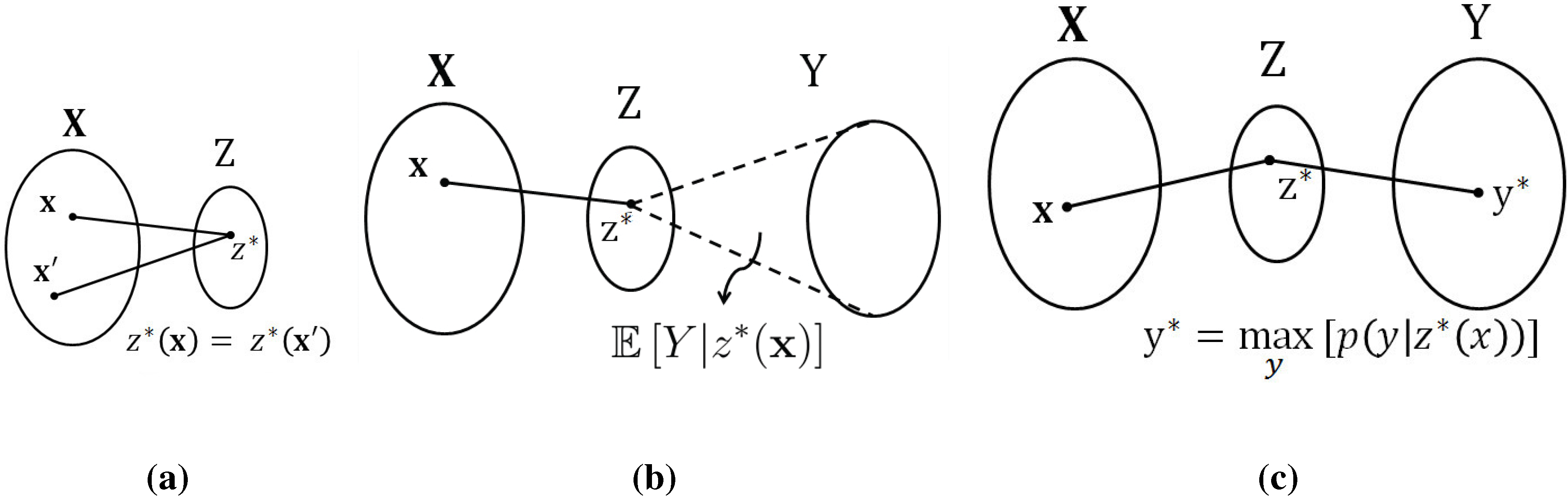
This problem does not appear to have a simple (algorithmic) solution. The key step enabling the method proposed in this paper is to (temporarily)
generalize the notion of a function. To this end, let us identify the function value with a new random variable
defined as follows:
At this point, it is natural to study the conditional probability distribution
. As long as we have
this conditional probability distribution is degenerate—
is equal to 1 whenever
and zero otherwise. Therefore, a tempting relaxation of the original problem is to optimize over
general conditional distributions
The next question is how to phrase the cardinality constraint in Equation (
2) in this new setting. Simply constraining the cardinality is not necessarily meaningful: it is acceptable for
Z to assume many different values, as long as most of them occur with small probability. Hence, an intuitively pleasing option might be to constrain the entropy
but this does not appear to lead to a tractable solution. Another option is to constrain the mutual information term
which can also be interpreted as capturing the compactness of the mapping (see Remark 1 below) and is sometimes referred to as the
compression-information. Thus, we arrive at the following formulation:
This formulation is precisely the problem known as the IB method. There exist several algorithms to solve for the maximizing conditional distribution
see e.g., [
17].
Remark 1
(Intuitive Interpretation of
as Compactness). Using the Asymptotic Equipartition Property (AEP) [
16], the probability
assigned to an observed input will be close to
and the total number of (typical) inputs is
. In that sense,
can be seen as the
volume of
. Also, for each (typical) value
z of
Z, there are
possible
input values which map to
z, all of which are equally likely. To ensure that no two input vectors map to the same
z, the set of possible inputs
has to be divided into subsets of size
, where each subset corresponds to a different value of
Z. Thus, the average cardinality of the mapping (partition) of
is given by the ratio of the volume of
to that of the mean partition:
By this reasoning, the quantity can be intuitively seen as a measure of compactness of Z. Lower values of correspond to a more compact Z and higher values for correspond to higher cardinalities of the functional mapping between and Z.
Remark 2
(Limitation of Information Measures for Function Identification). Define
as follows:
where
is a uniquely invertible one-to-one mapping and
is a constant.
For any defined in such a way, . This result is trivial for the case where all the involved variables are discrete as there would be a one-to-one mapping between (the support set or alphabet of Z) and (the alphabet of ), making and thus . This result also holds true for the continuous case due to the following argument:
If
is a
homeomorphism (smooth and uniquely invertible map) of
Z and
is the Jacobian determinant of the transformation, then
which gives
This result implies that tackling the function estimation problem using an approach involving mutual information cannot uniquely determine the function we are after. The solution we can expect to obtain is a class of equivalent functions that can be transformed from one to another through uniquely invertible maps.
5. Results on Artificial Data: Remapped-Linear Functions
In this section, we apply the proposed algorithms to artificial data. In order to set the stage for the application to experimental data, presented in
Section 6 below, we consider an example where the data is integer-valued, and where we look for functions that are
integer linear combinations. Specifically, we consider the following joint probability mass function
We let the inputs
be independent of each other and uniformly distributed with support
, where
. Moreover, we let the output
Y be
where
W is an additive independent noise following the same distribution as the
s. Here
is an arbitrary permutation function on the support set (which we refer to as
alphabet in this paper, matching the standard terminology in the information-theoretic literature). We chose this complex model to test our method because other methods such as linear regression will also be able to identify the coefficients when it is a simple linear model without any outer unknown function.
In this modified linear function setting of randomly generated data, we investigate whether the algorithm outlined in
Section 4 can recover these coefficients
. While doing so, we set the cardinality
of the compressed variable required for the iterative IB algorithm, to be much smaller than the true cardinality
of
Y so as to retrieve a compact function.
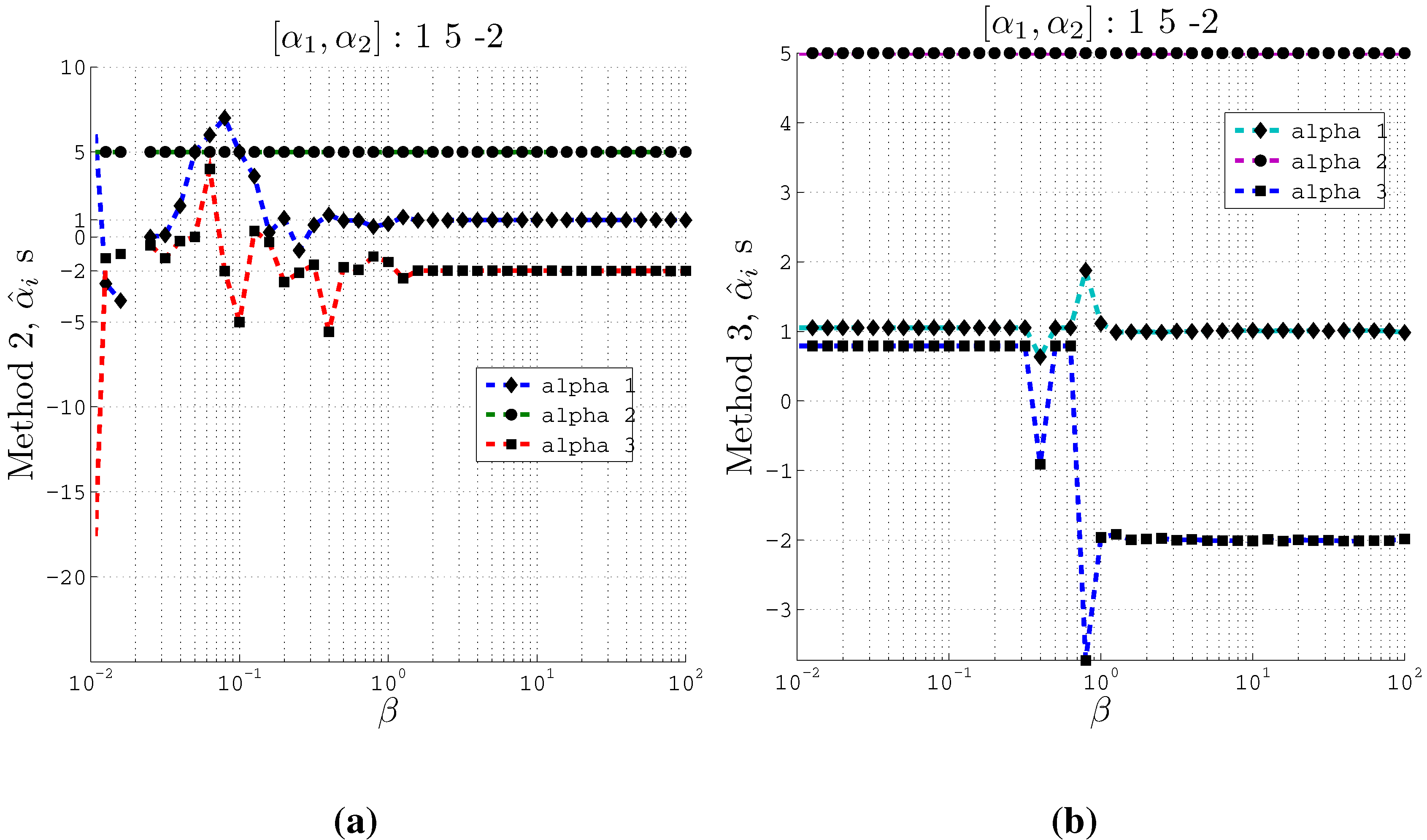
For example, consider the case when we have two inputs (
) with
and the actual coefficients
and
. Then the support of
and
becomes
. In this scenario the true cardinality
. We then run our algorithm for estimating the coefficients by setting
. As Methods 2 and 3 are more computationally efficient than Method 1, we focus on these two methods in the rest of the report.
Figure 3 plots the estimated normalized coefficients
and
for two inputs using both Method 2 and Method 3 at different values of the trade-off parameter
β. Similar plots are also depicted in
Figure 4 for three inputs with the same support and the actual coefficients set as
,
and
. In this case, the true cardinality
and the cardinality set in the IB algorithm
.
Figure 3.
Estimating coefficients and using Methods 2 and 3 on artificial data with 2 inputs of support at different values of the β parameter used in the IB algorithm. Here , and . (a) Using Method 2; (b) Using Method 3.
Figure 3.
Estimating coefficients and using Methods 2 and 3 on artificial data with 2 inputs of support at different values of the β parameter used in the IB algorithm. Here , and . (a) Using Method 2; (b) Using Method 3.
Figure 4.
Estimating coefficients and using Methods 2 and 3 on artificial data with 3 inputs of support at different values of the β parameter used in the IB algorithm. Here , and . (a) Using Method 2; (b) Using Method 3.
Figure 4.
Estimating coefficients and using Methods 2 and 3 on artificial data with 3 inputs of support at different values of the β parameter used in the IB algorithm. Here , and . (a) Using Method 2; (b) Using Method 3.
From these plots (
Figure 3 and
Figure 4) we observe that at relatively small
β values, the estimated
s converge to the actual coefficients
s even when the cardinality is set such that
. Moreover, Method 2 and Method 3 converge to the actual coefficients in different ways. Method 2 fluctuates greatly at very small
β values before it converges to the actual coefficient values. On the other hand, Method 3 is stable at small
β values and at a particular
β value, it converges to the actual coefficients.
Furthermore, the Θ values computed at different values of β correspond to the recovery of the original coefficients. At the values of β where the estimated coefficients become close to the original coefficients, we obtain high values for Θ. We observe a gradual increase of Θ value for increasing values of β. For example, in the 2 input case, using method 2, at , the computed Θ value is 1.347 which is high enough to accept the estimated coefficients from our algorithm. Similar high values for Θ are obtained for the 3 input case as well.
5.1. Comparison with Linear Regression and Related Model-Based Approaches
When parsing the compact representation Z to an actual function exhibiting simple mathematical structure, we restricted attending to linear functions in the present paper. It is therefore tempting to compare to methods that start out with a linear model from scratch (rather than bringing it in at the end, as we are doing in the proposed method). For example, consider linear regression: Given data from the considered three neurons, we could simply run linear regression for y based on and and this would provide us with the regression coefficients. This appears to be a much more direct and simpler approach to the function identification problem.
However, there is a significant downside to this approach: it requires one to separately impose how information is represented in absolute terms, with respect to the real numbers and mean-squared error. This information is crucially exploited by linear regression, though such a feature appears to violate the spirit of the function identification problem: functional behavior should be relative, not connected to absolute representations.
To illustrate this issue more concretely, the remapped-linear case is instructive. That is, suppose that the underlying ground truth is given by
It should be immediately obvious that linear regression will fail when applied directly to this data. Indeed, using the probability distribution leading to
Figure 3 and generating data from that distribution, linear regression returns the coefficients 912 and 1,045, which are very far from the true coefficients, 1 and 2 (not surprisingly).
6. Results on Experimental Data: Linear Function
6.1. Data Description
In this experiment, an adult male rhesus monkey (Macaca mulatta) performs a behavioral task for a duration of about 15 minutes (1,080,353 milliseconds, to be precise), while the resulting voltage traces are simultaneously measured in the primary motor cortex (M1) region of the brain using 64 Teflon-coated tungsten multielectrodes (35 μm diameter, 500 μm electrode spacing, in 8 by 8 configuration: CD Neural Engineering, Durham, NC, USA). The arrays were implanted bilaterally in the hand/arm area of M1, positioned at a depth of 3 mm targeting five pyramidal neurons. Localization of target areas was performed using stereotactic coordinates of the rhesus brain. We then use a low-pass filtered version of these voltage traces to obtain the neural responses from 184 neurons.
The monkey was trained to perform a delayed center-out reaching task using his right arm. The task involved cursor movements from the center toward one of eight targets distributed evenly on a 14-cm diameter circle. Target radius was set at 0.75 cm. Each trial began with a brief hold period at the center target, followed by a GO cue (center changed color) to signal the reach toward the target. The monkey was then required to reach and hold briefly (0.2–0.5 s) at the target in order to receive a liquid reward. Reaching was performed using a Kinarm (BKIN Technologies, Kingston, ON, Canada) exoskeleton where the monkey’s shoulder and elbow were constrained to move the device on a 2D plane. Over the course of the entire experiment, the reaching task is performed in different directions: , etc. Moreover, the reaching task in a particular direction is repeated several times; for example, the reaching task is repeated 36 times at different starting points in the entire duration of 15 minutes.
All procedures were conducted in compliance with the National Institutes of Health Guide for the Care and Use of Laboratory Animals and were approved by the University of California at Berkeley Institutional Animal Care and Use Committee.
6.2. Applying the Proposed Algorithm on Data
The functional identification algorithm outlined in
Section 4 is applied on this dataset to infer some structure present in the data. Before doing that, we first need to decide how to estimate the required probability distributions
from the data. Additionally, we also need to decide a way to deal with the temporal aspect of the neural spike trains from different neurons.
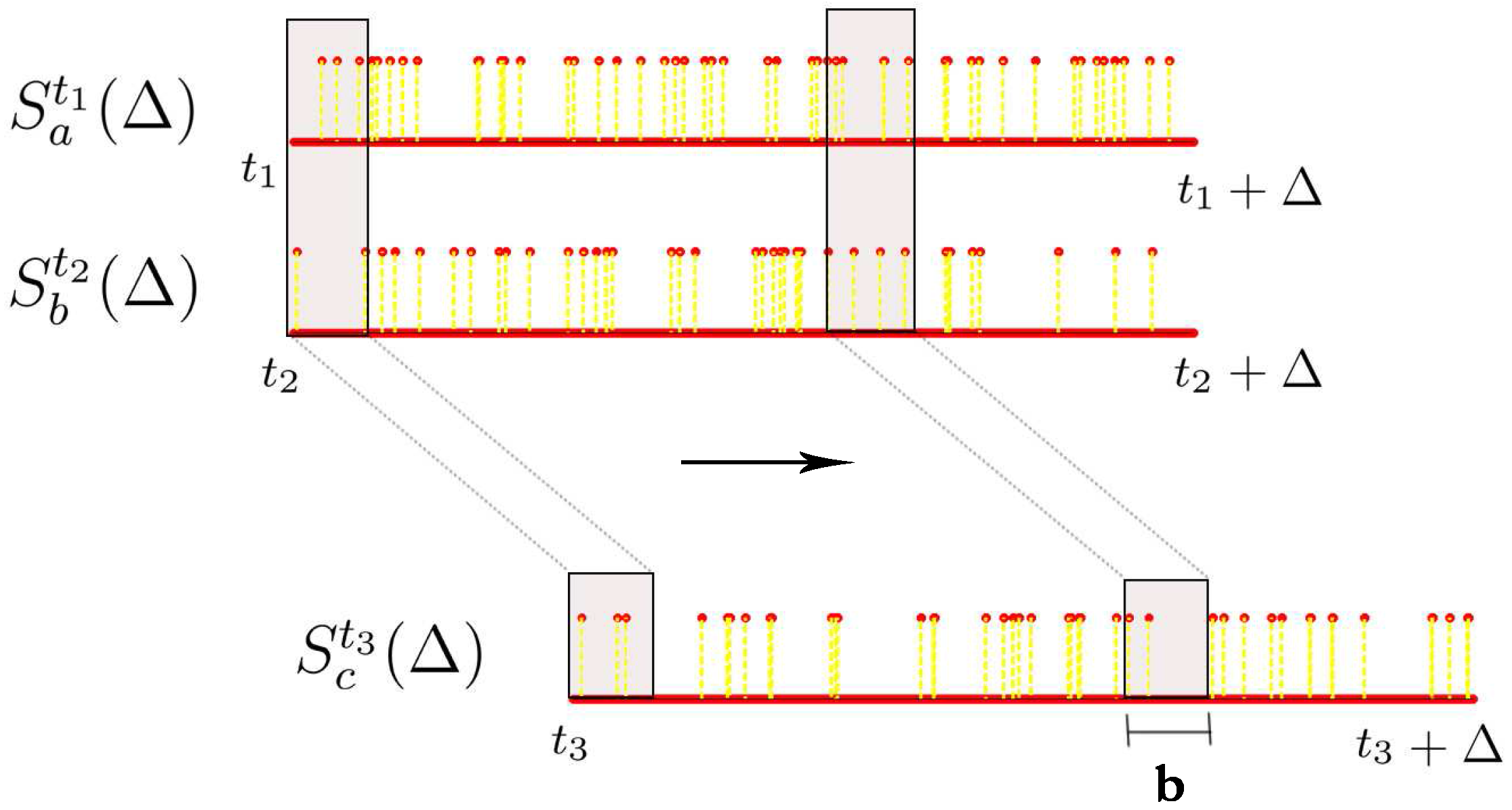
Let denote the spike train of neuron i starting from time t and lasting for Δ milliseconds, i.e., we are looking at the neural response of neuron with id i from time t ms to ms with a millisecond precision. can be seen as a vector of length Δ comprising of 0s and 1s where 0 represents no spike and 1 represents a spike. The number of spikes we have in this time window is denoted by .
Then a random variable. denoted by
, is estimated from
in the following way (
b here, is a binning parameter): c the histogram of the realizations
given by:
and normalize this histogram to get the probability distribution
. In other words, this procedure maintains a sliding window of length
b ms starting from the beginning of the spike train
, counts the number of spikes in this window while stepping this window to the right until we reach the end of the spike train
and normalizes this binned histogram to obtain the probability distribution of the random variable
(
Figure 5). Accordingly, the support of this random variable is the number of spikes observed in any contiguous segment of length
b ms of the spike train
.
The above procedure can be extended for estimating the joint probability distribution from multiple spike trains. In this project, we restrict ourselves to the case where given two spike train segments
and
, we want to know if there exists a linear functional relationship between these two spike train segments in order to explain a third spike train segment
. Therefore, we need to estimate the joint probability distribution of the three random variables
associated with these three spike train segments. To do this, we ensure that the sliding window is appropriately aligned across all these three spike trains while obtaining the joint histogram. This procedure is illustrated in
Figure 5. Once we have this joint histogram we can use the procedure outlined earlier in this chapter to estimate
and
such that the below functional relationship holds:
and
are the input random variables (
, as in the notation used in
Section 3) and
is the output random variable (
Y). It should be noted that we should expect to be able to identify such a relationship only occasionally from the data, as neurons generally do not behave in a predictable and deterministic way. We need to perform an exhaustive search to find the
right neurons (
), the time frames (
) when these neurons have interesting behaviors and also the suitable parameters Δ and
b for which such relationships exist and can be identified by our method. Accordingly, in order to reduce the search space, we assume that the two inputs neuron spike trains are aligned and start at the same time,
i.e.,
. We then try different delays
δ in the output neuron spike train,
i.e.,
and
.
Figure 5.
Estimating joint histograms from spike trains, where we consider overlapping bins using a sliding window.
Figure 5.
Estimating joint histograms from spike trains, where we consider overlapping bins using a sliding window.
6.3. Functions Identified in Data
Consider a particular trial of the
experiment which lasts from time 40,718 ms to time = 43,457 ms. The two input neuron spike trains are set to start at the advent of different events (like: center appears, hand enters center, go cue, hand enters target,
etc.) and the output neuron spike train is set to start at different delay values with respect to the input neurons with a maximum delay of 800 ms. We set the parameters for obtaining the joint histograms as
ms,
ms and the threshold
θ is set to 1.25. Below are a few functions obtained at the event when
hand enters center at time
of this experimental trial. For the sake of simplicity, we drop the superscript for the random variables corresponding to the input neurons with the understanding that both the input neuron spike trains start at
. Also, in the superscript of the output neuron’s random variable, we indicate only the delay
δ with respect to the input neurons. As it turned out,
all the functions we found were direct, unweighted sums. The functions are sorted in the descending order of the confidence parameter Θ.
with .
with .
with .
with .
with .
We observe that most of the normalized linear coefficients estimated by our method on this dataset are equal to 1, with rare occurrences of 2, and no values greater than 2. An example of such a weighted function was found between neurons 63, 114, and 28 in the case where we set the input spike trains to start at the event when the
hand enters the target (at time 42,705 ms) as given below:
However, such weighted functions were not frequently identified. This can be explained by looking at the support of the different random variables estimated from the spike trains. These supports are compact and concentrated in a particular range for most of the spike trains. Therefore, we do not observe higher normalized coefficient estimates such as 3 or 4. Functions at different events for different experimental trials can be identified in a similar way.
In order to better validate the results obtained using our proposed algorithm, we need to verify whether the functional relationships listed above are replicated in different trials of the same experiment. The next paragraph goes through a particular case study where the functional relationships between a particular triplet of neurons are analyzed over different trails of the same experiment.
Consider the following three neurons: 28, 114 and 98, with neurons 28 and 114 as the input neurons and neuron 98 as the output neuron. We want to observe the behavior of these three neurons across all 36 trials of the
reaching tasks. Out of these 36 trials, only 26 are as successful and the rest are considered unsuccessful as the monkey’s hand leaves the center before the go cue is given. The functional relationships obtained from one of the 26 successful trials that lasts from
ms to
ms were listed above. Let us look at one particular function, namely, the second item on the previous list:
The functional relationship in this equation implies that the sum of neuron 28 and neuron 114 at time 41,080 (which corresponds to the action of the hand entering center) is equal to neuron 98 after a delay of 370 ms. If we consider this as a reference trial, we are interested in knowing if a similar function exists between these neurons during other trials at this delay of 370 ms (which corresponds to when the hand enters center).
Accordingly, we apply this above function obtained between neurons (28,114,98) during this reference trial, at identical stages of the different trials of the
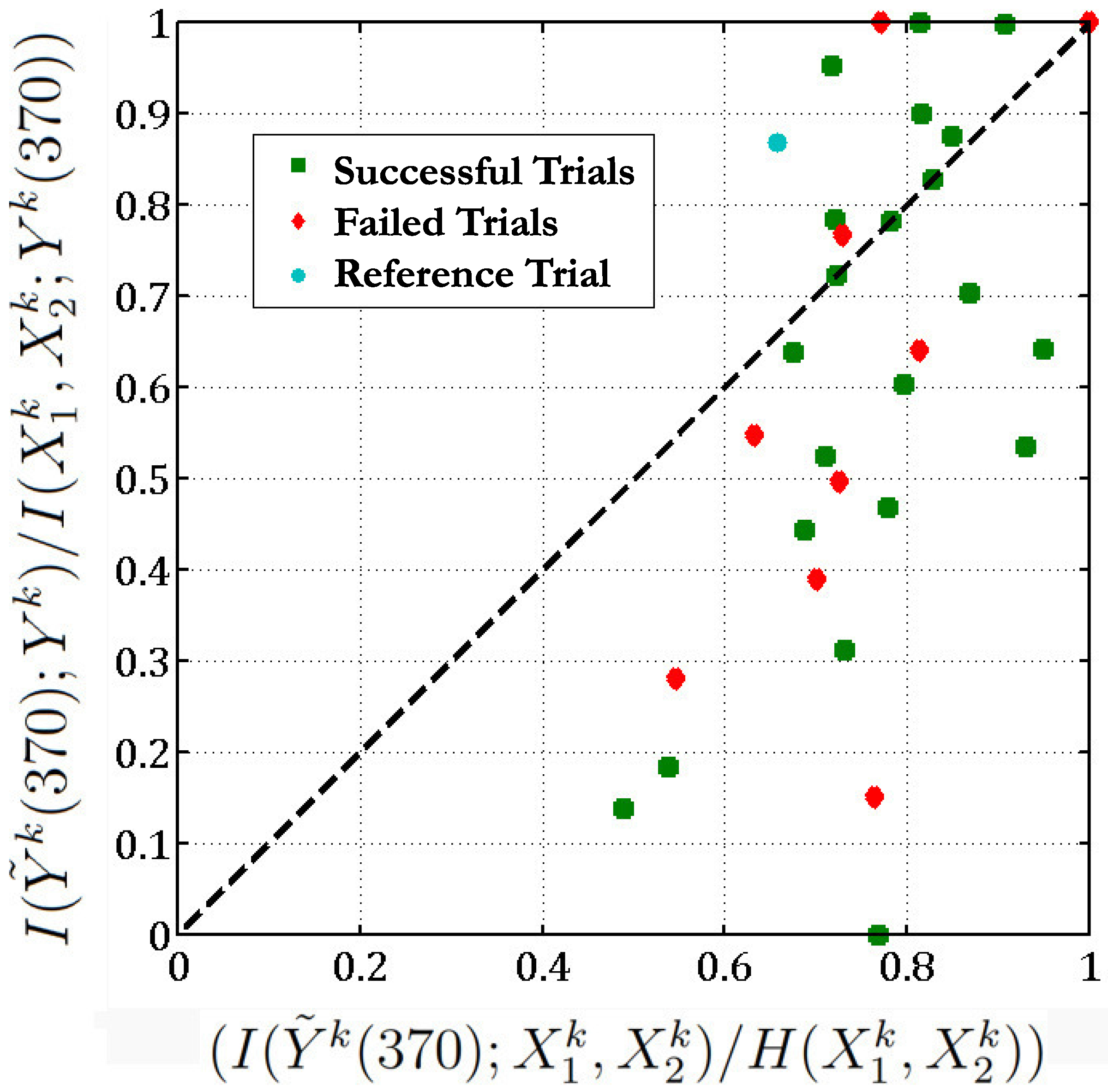
reaching task. There are 36 such trials in the same direction. We then plot
versus , for all these scenarios (
Figure 6). Here
,
are the 2 input neurons (28 and 114) starting at time
t where the hand enters the center for trial
k and
is the variable corresponding to the output neuron (98) in trial
k after a delay of 370 ms w.r.t the input neurons. Here,
is computed as described in
Section 4.3 from the estimated coefficients in order to check for sufficient evidence for the function found between
.
Figure 6.
We check if the function (Equation (
37)) obtained between neurons 28, 114 and 98 in the reference trial (t = 40,718) is valid across all 36 trials of the
reaching task with a threshold
.
Figure 6.
We check if the function (Equation (
37)) obtained between neurons 28, 114 and 98 in the reference trial (t = 40,718) is valid across all 36 trials of the
reaching task with a threshold
.
Figure 6 implies that in 13 out of the 36 different trials of the
reaching task, the
sum of neurons 28 and 114 is equal to the response of neuron 98 as the points corresponding to these trials lie above the
line (here we set the threshold
). In one-third of the experimental trials, the functional relationship given in Equation (
37) holds. Moreover, if we exclude the unsuccessful trials, then 10 out of 26 of the successful trials follow the above functional relationship between neurons 28, 114 and 98. Most of the unsuccessful trials lie below the
line (
) which indicates that these neurons behave in a different manner during an unsuccessful trial. The below table lists the Θ values corresponding to all the trials (we exclude 5 trials which give Θ of the form
and
):
| Successful Trials | Unsuccessful Trials |
| | | |
| 1.331 | 0.947 | 1.000 | 0.197 |
| 1.321 | 0.811 | 1.052 | 0.513 |
| 1.229 | 0.758 | 1.293 | 0.555 |
| 1.114 | 0.739 | | 0.685 |
| 1.109 | 0.676 | | 0.787 |
| 1.102 | 0.647 | | 0.865 |
| 1.091 | 0.601 | | |
| 1.000 | 0.574 | | |
| 1.000 | 0.427 | | |
| 1.000 | 0.341 | | |
| | 0.283 | | |
| | 0.000 | | |
For successful trials, we can consider the cases when
as
true positives (TP) and the cases when
as
false negatives (FN). Similarly for the unsuccessful trials, we can consider the cases when
as
false positives (FP) and the case when
as
true negatives (TN). Then, at this value of the threshold
we can compute the following quantities:
True Positive Rate (TPR) = TP/(TP+FP) = 76.92%
True Negative Rate (TNR) = TN/((TN+FN) = 33.33%
Sensitivity = TP/(TP+FN) = 45.45%
Specificity = TN/(TN+FP) = 66.67%
We achieve high TPR but not such a high TNR as there are many false negatives. It should be noted that these values depend on the value of the threshold
θ. These numbers indicate that the functions identified by our algorithm in a particular trial are somewhat consistent across different trials of the reaching task of the same type.


