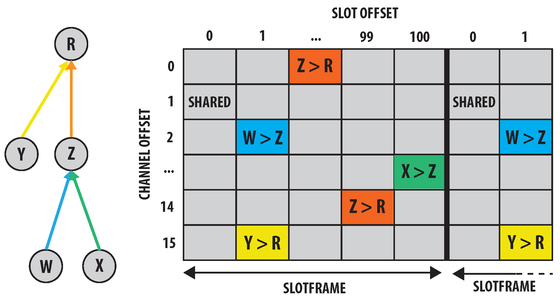
Figure 1.
TSCH schedule example.
Figure 1.
TSCH schedule example.
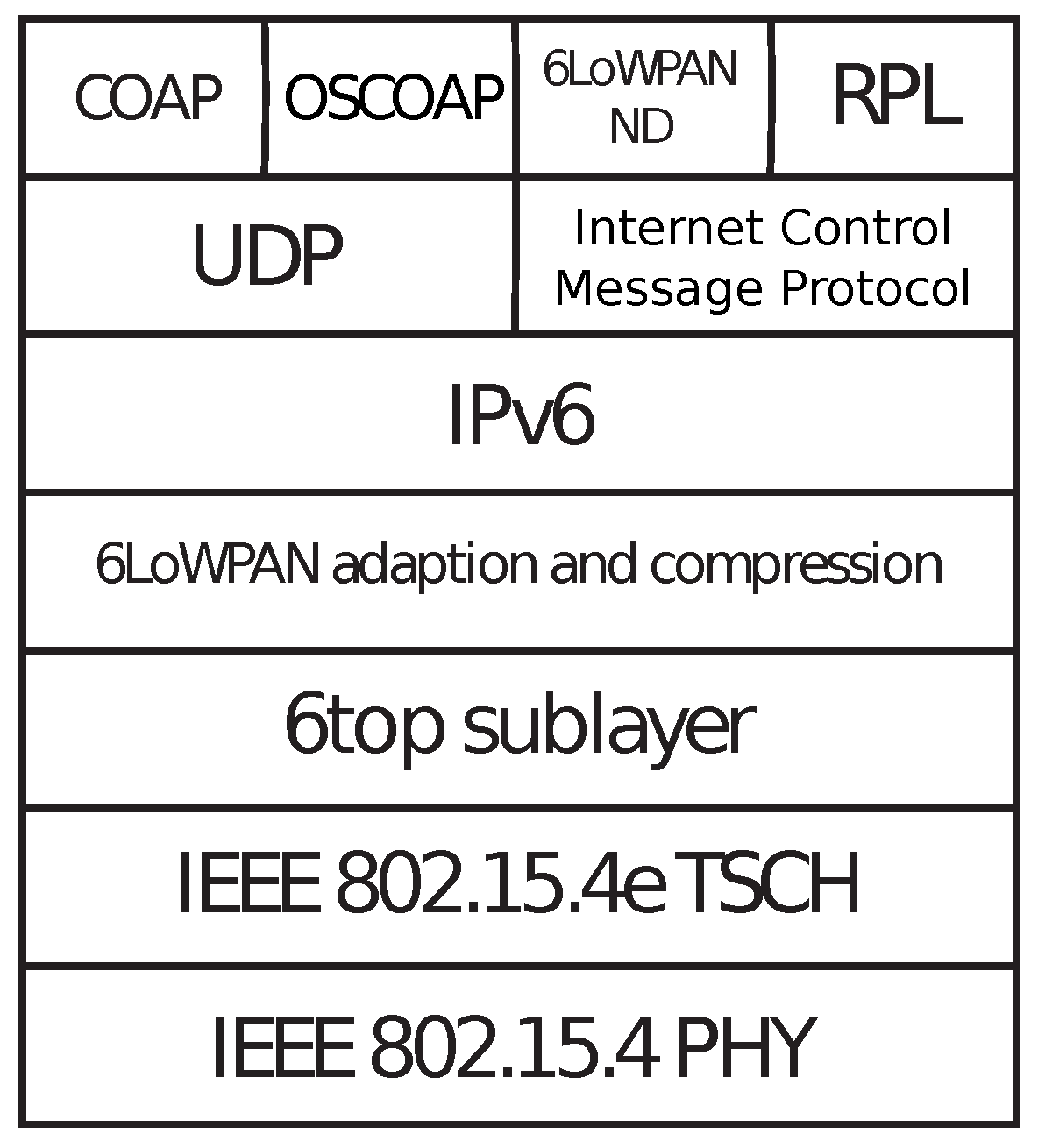
Figure 2.
The IPv6 over the TSCH mode of IEEE 802.15.4e (6TiSCH) architecture stack. RPL, Routing Protocol for Low-power and Lossy network.
Figure 2.
The IPv6 over the TSCH mode of IEEE 802.15.4e (6TiSCH) architecture stack. RPL, Routing Protocol for Low-power and Lossy network.
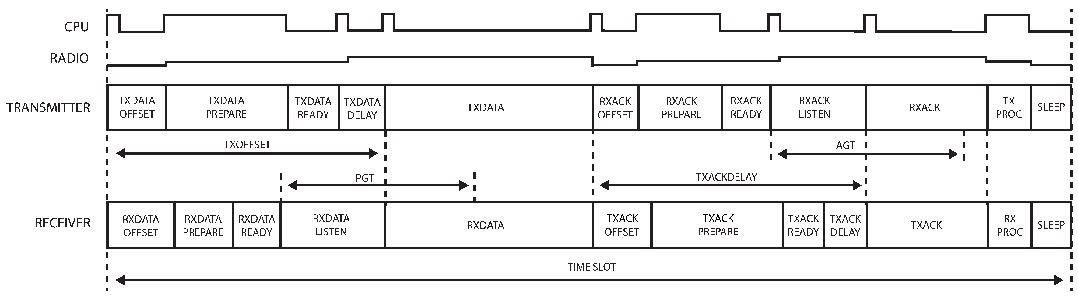
Figure 3.
States in TxDataRxAck (transmitter) and RxDataTxAck (receiver) time slots, together with the CPU and radio activity in the TxDataRxAck time slot.
Figure 3.
States in TxDataRxAck (transmitter) and RxDataTxAck (receiver) time slots, together with the CPU and radio activity in the TxDataRxAck time slot.
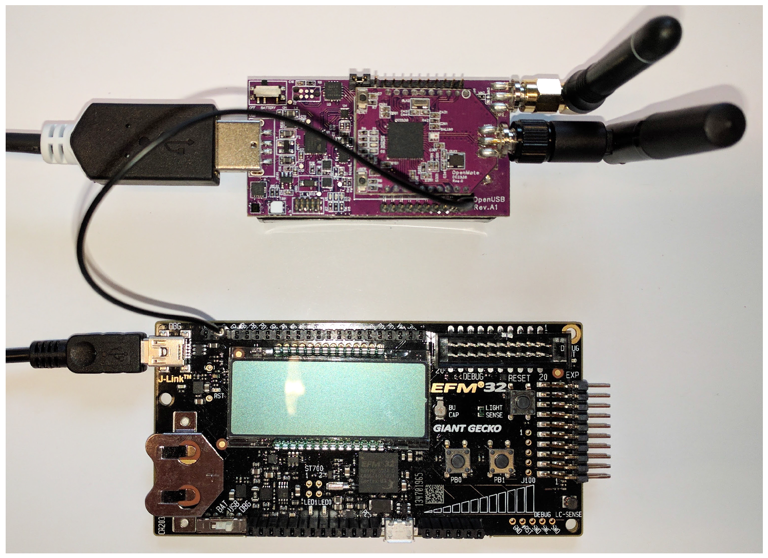
Figure 4.
Setup used to measure state durations with a connection from the PB9 pin on the Gecko board (bottom) and to the PD2 pin on the OpenUSB (top).
Figure 4.
Setup used to measure state durations with a connection from the PB9 pin on the Gecko board (bottom) and to the PD2 pin on the OpenUSB (top).
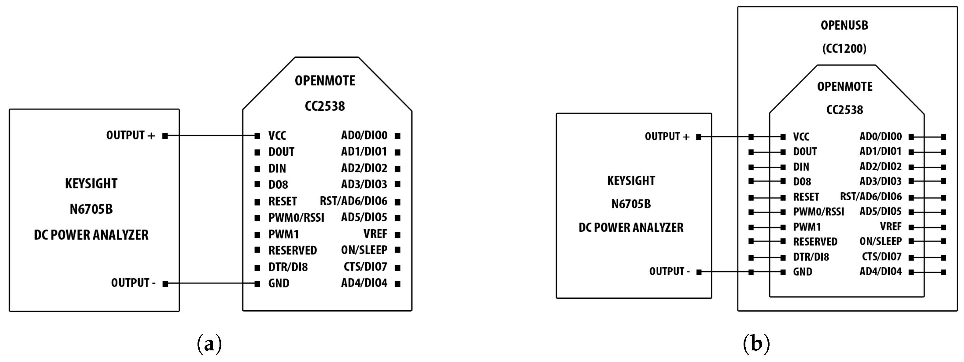
Figure 5.
Energy consumption measurement setups: for the GHz measurements, only the OpenMote-CC2538 was used, while for the 868 GHz measurements, the power analyzer was connected to the OpenUSB to which the OpenMote-CC2538 was attached. (a) 2.4 GHz measurement setup; (b) 868 MHz measurement setup.
Figure 5.
Energy consumption measurement setups: for the GHz measurements, only the OpenMote-CC2538 was used, while for the 868 GHz measurements, the power analyzer was connected to the OpenUSB to which the OpenMote-CC2538 was attached. (a) 2.4 GHz measurement setup; (b) 868 MHz measurement setup.
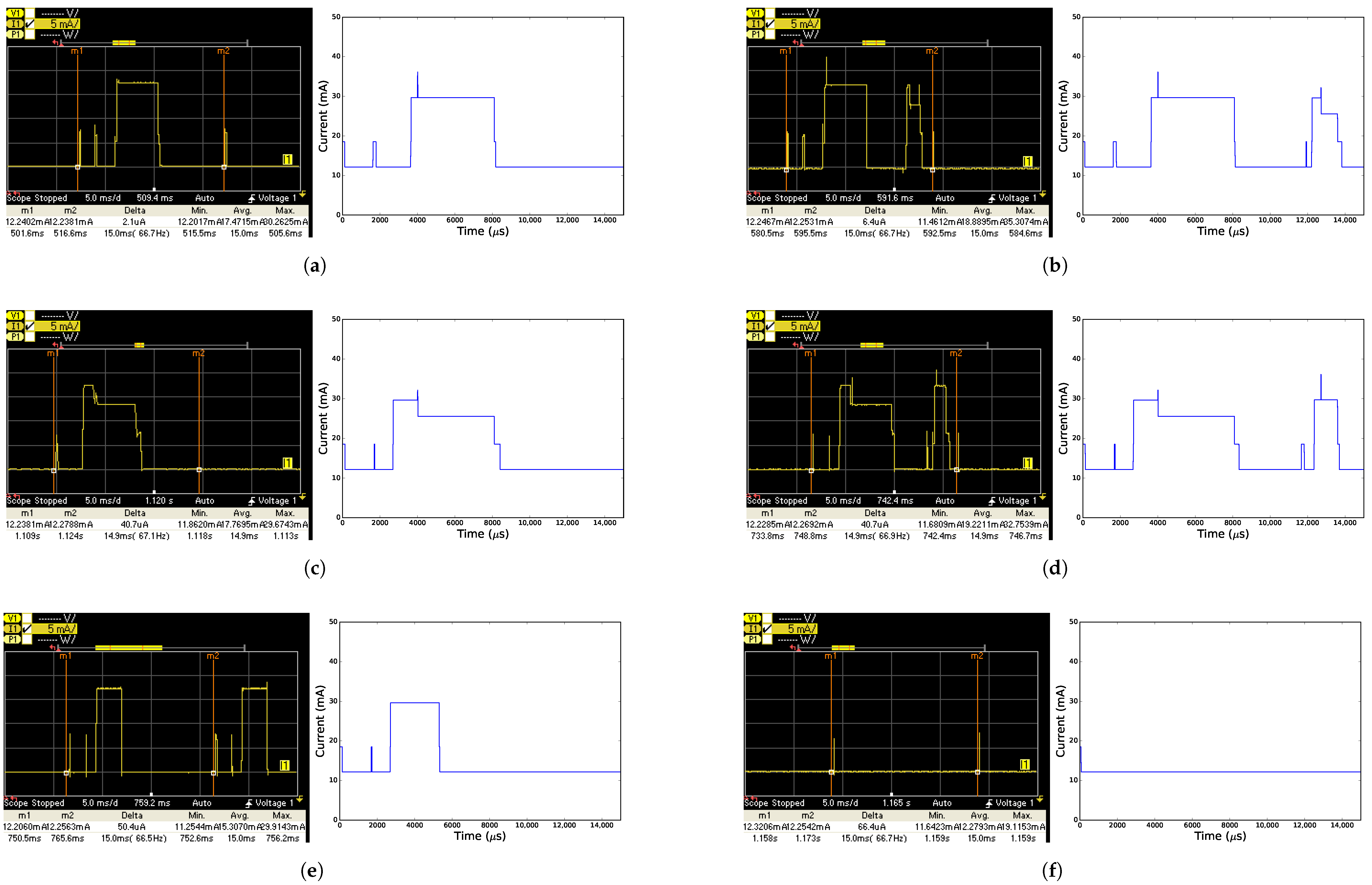
Figure 6.
Measured (left, between vertical lines m1 and m2) and modeled (right) current comparison for each time slot when using the CC2538 radio. (a) TxData time slot; (b) TxDataRxAck time slot; (c) RxData time slot; (d) RxDataTxAck time slot; (e) RxIdle time slot; (f) Sleep time slot.
Figure 6.
Measured (left, between vertical lines m1 and m2) and modeled (right) current comparison for each time slot when using the CC2538 radio. (a) TxData time slot; (b) TxDataRxAck time slot; (c) RxData time slot; (d) RxDataTxAck time slot; (e) RxIdle time slot; (f) Sleep time slot.
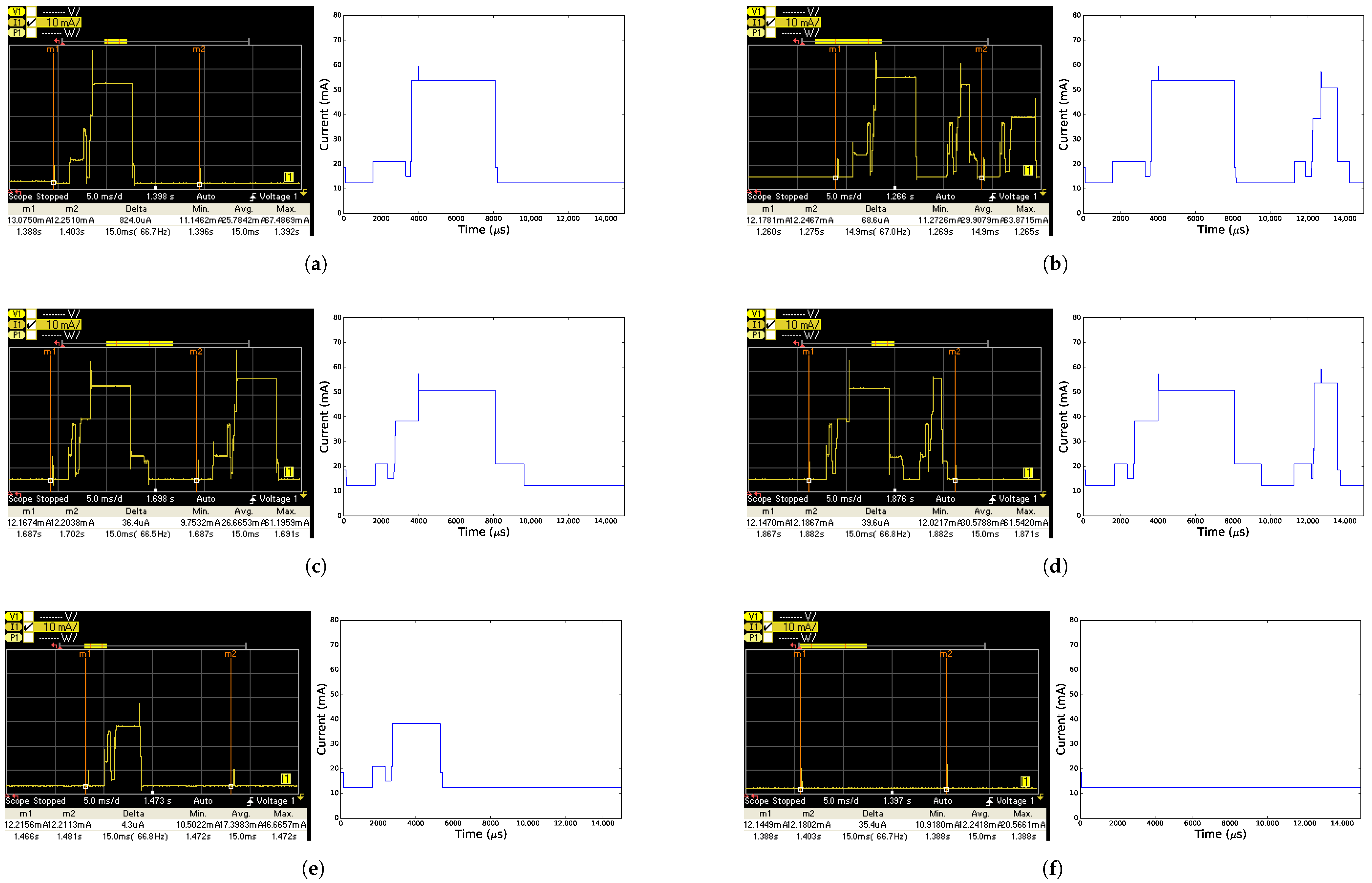
Figure 7.
Measured (left, between vertical lines m1 and m2) and modeled (right) current comparison for each time slot when using the CC1200 radio. (a) TxData time slot; (b) TxDataRxAck time slot; (c) RxData time slot; (d) RxDataTxAck time slot; (e) RxIdle time slot; (f) Sleep time slot.
Figure 7.
Measured (left, between vertical lines m1 and m2) and modeled (right) current comparison for each time slot when using the CC1200 radio. (a) TxData time slot; (b) TxDataRxAck time slot; (c) RxData time slot; (d) RxDataTxAck time slot; (e) RxIdle time slot; (f) Sleep time slot.
Figure 8.
Topology used while comparing the consumption of a slot frame.
Figure 8.
Topology used while comparing the consumption of a slot frame.
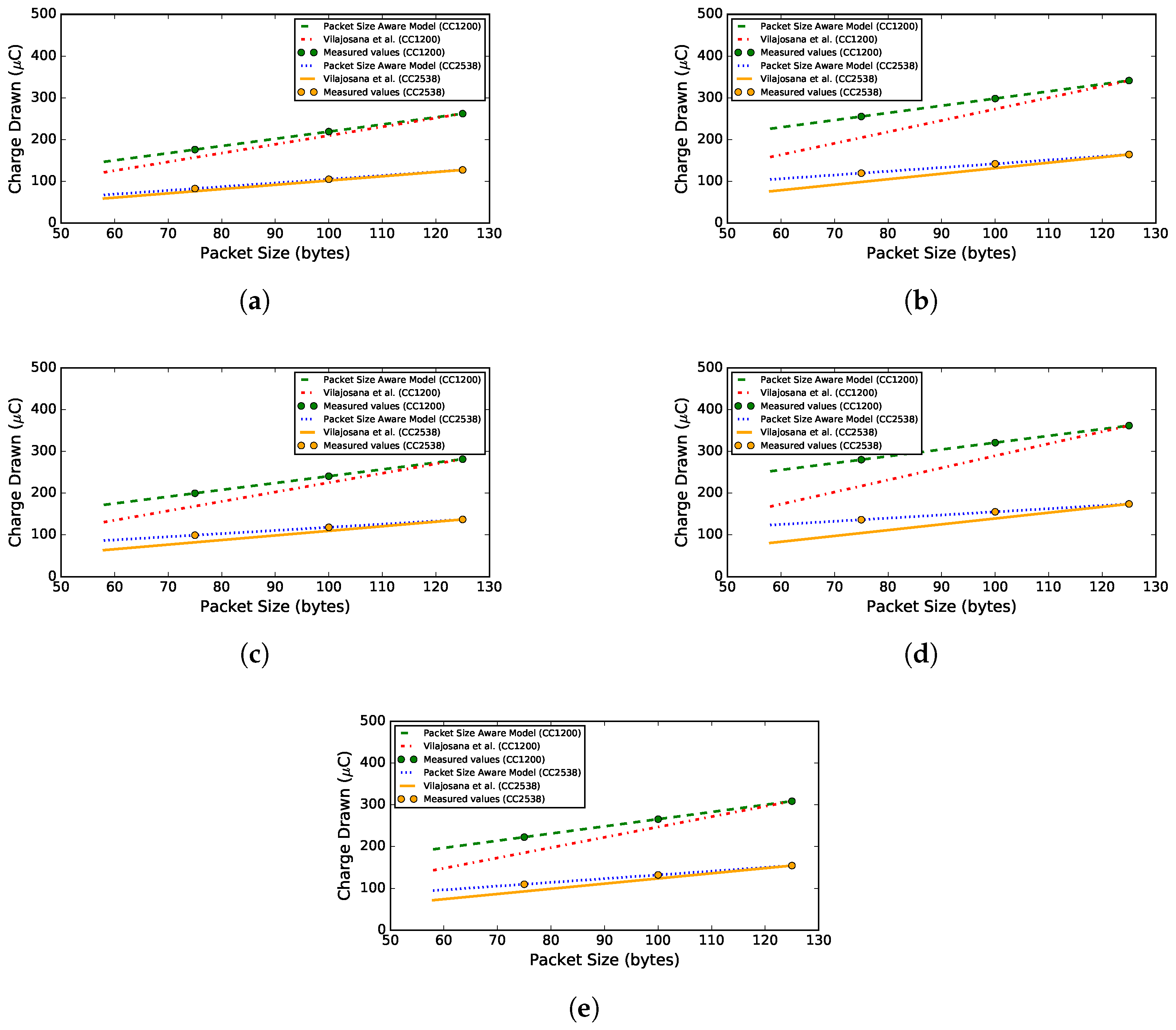
Figure 9.
Comparison between the proposed packet size aware model and the model introduced by Vilajosana et al., which linearly scales the charge consumption based on the packet size. (a) TxData time slot; (b) TxDataRxAck time slot; (c) RxData time slot; (d) RxDataTxAck time slot; (e) TxDataRxNoAck time slot.
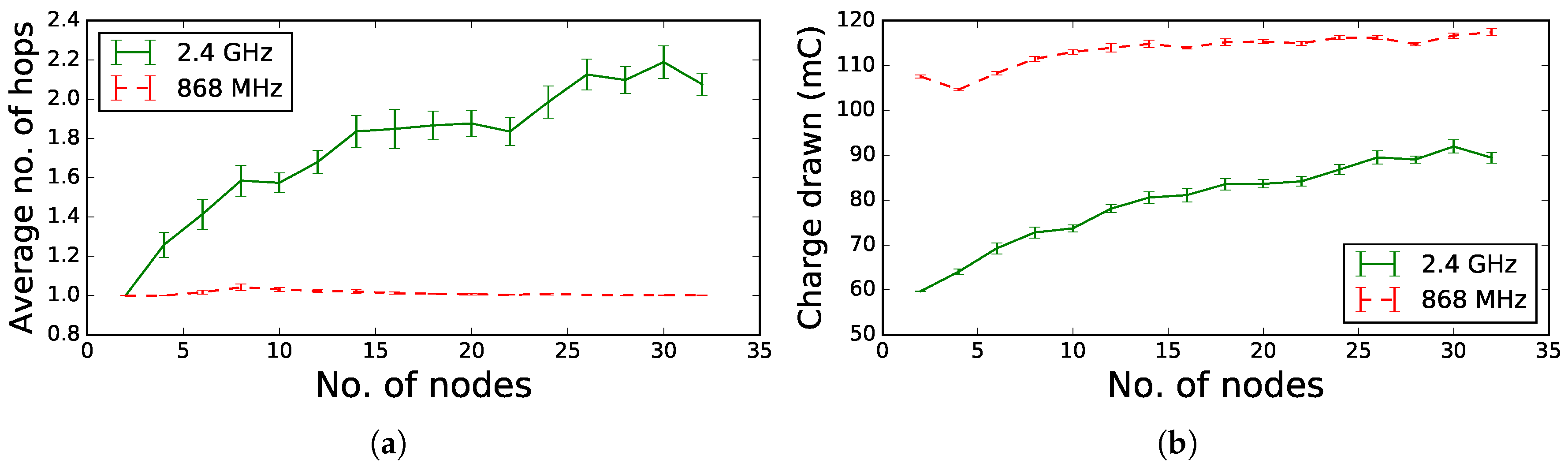
Figure 10.
Total consumed charge per node and average hop count for 868 MHz and 2.4 GHz frequency communication in a random topology as a function of the number of nodes. (a) Average hop count; (b) total energy consumed per node.
Figure 10.
Total consumed charge per node and average hop count for 868 MHz and 2.4 GHz frequency communication in a random topology as a function of the number of nodes. (a) Average hop count; (b) total energy consumed per node.
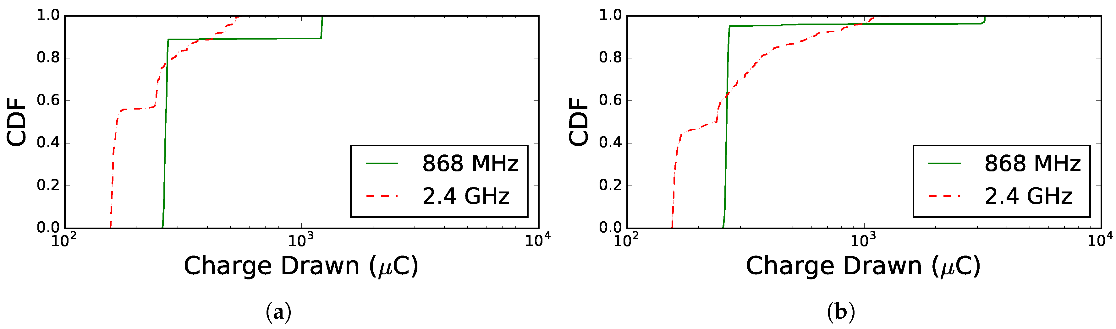
Figure 11.
Comparison of charge drawn per cycle per node for 868 MHz and 2.4 GHz frequency communication in a grid topology of nine nodes and 25 nodes. (a) Grid topology of nine nodes; (b) grid topology of 25 nodes.
Figure 11.
Comparison of charge drawn per cycle per node for 868 MHz and 2.4 GHz frequency communication in a grid topology of nine nodes and 25 nodes. (a) Grid topology of nine nodes; (b) grid topology of 25 nodes.
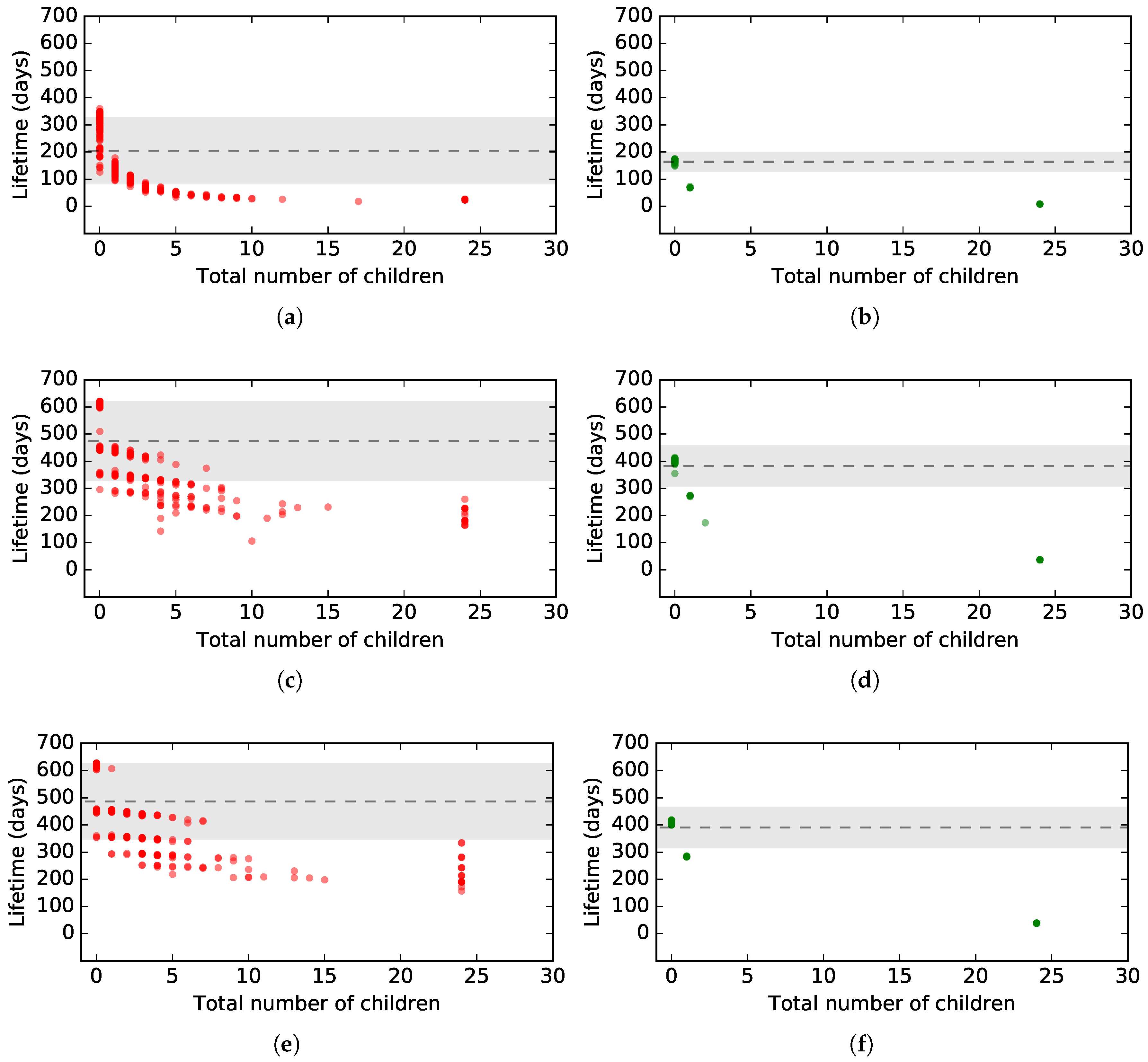
Figure 12.
Comparison of the lifetime of a TSCH node, running on two AA batteries, between 2.4 GHz and 868 MHz communication for different packet periods in a grid topology of 25 nodes. (a) 1 packet/s, 2.4 GHz; (b) 1 packet/s, 868 GHz; (c) 1 packet/min, 2.4 GHz; (d) 1 packet/min, 868 GHz; (e) 1 packet/h, 2.4 GHz; (f) 1 packet/h, 868 GHz.
Table 1.
States in a TxDataRxAck slot.
Table 1.
States in a TxDataRxAck slot.
| State | CPU State | Radio State |
|---|
| TxDataOffsetStart | Active | Sleep |
| TxDataOffset | Sleep | Sleep |
| TxDataPrepare | Active | Idle |
| TxDataReady | Sleep | Idle |
| TxDataDelayStart | Active | Idle |
| TxDataDelay | Sleep | TX |
| TxDataStart | Active | TX |
| TxData | Sleep | TX |
| RxAckOffsetStart | Active | Sleep |
| RxAckOffset | Sleep | Sleep |
| RxAckPrepare | Active | Idle |
| RxAckReady | Sleep | Idle |
| RxAckListenStart | Active | Idle |
| RxAckListen | Sleep | Listen |
| RxAckStart | Active | RX |
| RxAck | Sleep | RX |
| TxProc | Active | Idle |
| Sleep | Sleep | Sleep |
Table 2.
States in a RxDataTxAck slot.
Table 2.
States in a RxDataTxAck slot.
| State | CPU State | Radio State |
|---|
| RxDataOffsetStart | Active | Sleep |
| RxDataOffset | Sleep | Sleep |
| RxDataPrepare | Active | Idle |
| RxDataReady | Sleep | Idle |
| RxDataListenStart | Active | Idle |
| RxDataListen | Sleep | Listen |
| RxDataStart | Active | RX |
| RxData | Sleep | RX |
| TxAckOffsetStart | Active | Idle |
| TxAckOffset | Sleep | Sleep |
| TxAckPrepare | Active | Idle |
| TxAckReady | Sleep | Idle |
| TxAckDelayStart | Active | Idle |
| TxAckDelay | Sleep | TX |
| TxAckStart | Active | TX |
| TxAck | Sleep | TX |
| RxProc | Active | Sleep |
| Sleep | Sleep | Sleep |
Table 3.
States in a TxData slot.
Table 3.
States in a TxData slot.
| State | CPU State | Radio State |
|---|
| TxDataOffsetStart | Active | Sleep |
| TxDataOffset | Sleep | Sleep |
| TxDataPrepare | Active | Idle |
| TxDataReady | Sleep | Idle |
| TxDataDelayStart | Active | Idle |
| TxDataDelay | Sleep | TX |
| TxDataStart | Active | TX |
| TxData | Sleep | TX |
| TxProc | Active | Sleep |
| Sleep | Sleep | Sleep |
Table 4.
States in a RxData slot.
Table 4.
States in a RxData slot.
| State | CPU State | Radio State |
|---|
| RxDataOffsetStart | Active | Sleep |
| RxDataOffset | Sleep | Sleep |
| RxDataPrepare | Active | Idle |
| RxDataReady | Sleep | Idle |
| RxDataListenStart | Active | Idle |
| RxDataListen | Sleep | Listen |
| RxDataStart | Active | RX |
| RxData | Sleep | RX |
| RxProc | Active | Idle |
| Sleep | Sleep | Sleep |
Table 5.
States in a RxIdle slot.
Table 5.
States in a RxIdle slot.
| State | CPU State | Radio State |
|---|
| RxDataOffsetStart | Active | Sleep |
| RxDataOffset | Sleep | Sleep |
| RxDataPrepare | Active | Idle |
| RxDataReady | Sleep | Idle |
| RxDataListenStart | Active | Idle |
| RxDataListen | Sleep | Listen |
| RxProc | Active | Sleep |
| Sleep | Sleep | Sleep |
Table 6.
States in a Sleep slot.
Table 6.
States in a Sleep slot.
| State | CPU State | Radio State |
|---|
| SleepStart | Active | Sleep |
| Sleep | Sleep | Sleep |
Table 7.
States in a TxDataRxNoAck slot.
Table 7.
States in a TxDataRxNoAck slot.
| State | CPU State | Radio State |
|---|
| TxDataOffsetStart | Active | Sleep |
| TxDataOffset | Sleep | Sleep |
| TxDataPrepare | Active | Idle |
| TxDataReady | Sleep | Idle |
| TxDataDelayStart | Active | Idle |
| TxDataDelay | Sleep | TX |
| TxDataStart | Active | TX |
| TxData | Sleep | TX |
| RxAckOffsetStart | Active | Sleep |
| RxAckOffset | Sleep | Sleep |
| RxAckPrepare | Active | Idle |
| RxAckReady | Sleep | Idle |
| RxAckListenStart | Active | Idle |
| RxAckListen | Sleep | Listen |
| TxProc | Active | Sleep |
| Sleep | Sleep | Sleep |
Table 8.
State durations in the TxDataRxAck time slot with a total length of 15 ms and s being the packet size in bytes.
Table 8.
State durations in the TxDataRxAck time slot with a total length of 15 ms and s being the packet size in bytes.
| State | Duration (μs) |
|---|
| CC2538 | CC1200 |
| TxDataOffsetStart | 105 | 105 |
| TxDataOffset | 1515 | 1454 |
| TxDataPrepare | | |
| TxDataReady | | |
| TxDataDelayStart | 17 | 58 |
| TxDataDelay | 349 | 369 |
| TxDataStart | 16 | 16 |
| TxData | | |
| RxAckOffsetStart | 32 | 75 |
| RxAckOffset | 3769 | 3116 |
| RxAckPrepare | 38 | 587 |
| RxAckReady | 267 | 328 |
| RxAckListenStart | 17 | 58 |
| RxAckListen | 483 | 442 |
| RxAckStart | 16 | 15 |
| RxAck | 880 | 881 |
| TxProc | 225 | 619 |
| Sleep | | |
Table 9.
State durations in the Sleep time slot with a total length of 15 ms.
Table 9.
State durations in the Sleep time slot with a total length of 15 ms.
| State | Duration (μs) |
|---|
| CC2538 | CC1200 |
| SleepStart | 57 | 57 |
| Sleep | 14,943 | 14,943 |
Table 10.
State durations in the RxIdle time slot with a total length of 15 ms.
Table 10.
State durations in the RxIdle time slot with a total length of 15 ms.
| State | Duration (μs) |
|---|
| CC2538 | CC1200 |
| RxDataOffsetStart | 126 | 126 |
| RxDataOffset | 1567 | 1567 |
| RxDataPrepare | 38 | 676 |
| RxDataReady | 969 | 331 |
| RxDataListenStart | 17 | 58 |
| RxDataListen | 2583 | 2542 |
| RxProc | 25 | 118 |
| Sleep | 9675 | 9582 |
Table 11.
State durations in the RxDataTxAck time slot with a total length of 15 ms and s being the packet size in bytes.
Table 11.
State durations in the RxDataTxAck time slot with a total length of 15 ms and s being the packet size in bytes.
| State | Duration (μs) |
|---|
| CC2538 | CC1200 |
| RxDataOffsetStart | 126 | 126 |
| RxDataOffset | 1567 | 1567 |
| RxDataPrepare | 38 | 676 |
| RxDataReady | 969 | 331 |
| RxDataListenStart | 17 | 58 |
| RxDataListen | 1283 | 1242 |
| RxDataStart | 17 | 15 |
| RxData | | |
| TxAckOffsetStart | | |
| TxAckOffset | | |
| TxAckPrepare | 153 | 930 |
| TxAckReady | 518 | 77 |
| TxAckDelayStart | 17 | 58 |
| TxAckDelay | 349 | 369 |
| TxAckStart | 16 | 15 |
| TxAck | 880 | 881 |
| RxProc | 94 | 135 |
| Sleep | | |
Table 12.
State durations in the TxData time slot with a total length of 15 ms and s being the packet size in bytes.
Table 12.
State durations in the TxData time slot with a total length of 15 ms and s being the packet size in bytes.
| State | Duration (μs) |
|---|
| CC2538 | CC1200 |
| TxDataOffsetStart | 105 | 105 |
| TxDataOffset | 1515 | 1454 |
| TxDataPrepare | | |
| TxDataReady | | |
| TxDataDelayStart | 17 | 58 |
| TxDataDelay | 349 | 369 |
| TxDataStart | 16 | 16 |
| TxData | | |
| TxProc | 72 | 109 |
| Sleep | 10,832 | 10,795 |
Table 13.
State durations in the RxData time slot with a total length of 15 ms and s being the packet size in bytes.
Table 13.
State durations in the RxData time slot with a total length of 15 ms and s being the packet size in bytes.
| State | Duration (μs) |
|---|
| CC2538 | CC1200 |
| RxDataOffsetStart | 126 | 126 |
| RxDataOffset | 1567 | 1567 |
| RxDataPrepare | 38 | 676 |
| RxDataReady | 969 | 331 |
| RxDataListenStart | 17 | 58 |
| RxDataListen | 1283 | 1242 |
| RxDataStart | 17 | 15 |
| RxData | | |
| RxProc | | |
| Sleep | 10,706 | 10,416 |
Table 14.
State durations in the TxDataRxNoAck time slot with a total length of 15 ms and s being the packet size in bytes.
Table 14.
State durations in the TxDataRxNoAck time slot with a total length of 15 ms and s being the packet size in bytes.
| State | Duration (μs) |
|---|
| CC2538 | CC1200 |
| TxDataOffsetStart | 105 | 105 |
| TxDataOffset | 1515 | 1454 |
| TxDataPrepare | | |
| TxDataReady | | |
| TxDataDelayStart | 17 | 58 |
| TxDataDelay | 349 | 369 |
| TxDataStart | 16 | 16 |
| TxData | | |
| RxAckOffsetStart | 32 | 75 |
| RxAckOffset | 3769 | 3116 |
| RxAckPrepare | 38 | 587 |
| RxAckReady | 267 | 328 |
| RxAckListenStart | 17 | 58 |
| RxAckListen | 983 | 942 |
| TxProc | 44 | 137 |
| Sleep | | |
Table 15.
Current drawn during different device states.
Table 15.
Current drawn during different device states.
| CPU State | Radio State | Consumption (mA) |
|---|
| | CC2538 | CC1200 |
| Active | Sleep | 13.97 | 15.06 |
| Active | Idle | 13.97 | 17.49 |
| Active | Listen | 31.14 | 40.13 |
| Active | RX | 26.94 | 50.63 |
| Active | TX | 31.47 | 54.26 |
| Sleep (PM_NOACTION) | Sleep | 10.06 | 11.42 |
| Sleep (PM_NOACTION) | Idle | 10.06 | 13.82 |
| Sleep (PM_NOACTION) | Listen | 27.18 | 36.18 |
| Sleep (PM_NOACTION) | RX | 23.16 | 46.73 |
| Sleep (PM_NOACTION) | TX | 27.55 | 50.24 |
| Sleep (PM2) | Sleep | 0.00156 | 0.27 |
| Sleep (PM2) | Idle | 0.00156 | 2.64 |
Table 16.
Measured and calculated charge drawn for each slot type.
Table 16.
Measured and calculated charge drawn for each slot type.
| Slot Type | Measured (μs) | Calculated (μs) |
|---|
| CC2538 | CC1200 | CC2538 | CC1200 |
|---|
| TxDataRxAck | 250.35 | 420.01 | 250.94 | 407.81 |
| RxDataTxAck | 253.2 | 432.09 | 251.32 | 417.2 |
| TxData | 229.8 | 360.2 | 230.13 | 357.12 |
| RxData | 235.1 | 373.55 | 228.72 | 362.12 |
| RxIdle | 197.4 | 245.2 | 196.35 | 240.98 |
| Sleep | 152.4 | 168.65 | 151.12 | 171.51 |
| TxDataRxNoAck | 246.95 | 395.65 | 246.79 | 384.94 |
Table 17.
Measured and calculated charge drawn during a slot frame.
Table 17.
Measured and calculated charge drawn during a slot frame.
| Mote Type | Measured (μC) | Calculated> (μC) |
|---|
| CC2538 | CC1200 | CC2538 | CC1200 |
|---|
| Leaf (Sleep) | 7833.6 | 8698.05 | 7752.35 | 8816.48 |
| Leaf (TxDataRxAck) | 7910.1 | 8942.85 | 7852.17 | 9052.78 |
| Relay | 8086.05 | 9348.3 | 8002.81 | 9442.96 |
Table 18.
Parameter configuration in the 6TiSCH simulator.
Table 18.
Parameter configuration in the 6TiSCH simulator.
| Parameter | 868 MHz | 2.4 GHz |
|---|
| Timeslot duration | 15 ms |
| Slot frame size | 101 time slots |
| No. of SHARED cells | 1 |
| Inter-node distance | 70 m |
| No. of stable neighbors | 1 |
| RPL parent set size | 1 |
| Traffic period | 5 s |
| Traffic period variability | 0.05 |
| EB period | 10 s |
| EB probability | 0.15 s |
| DIO period | 30 s |
| DIO probability | 0.15 |
| OTF threshold | 2 |
| OTF housekeeping period | 10 s |
| 6top housekeeping | False |
| TX power | 0 dBm |
| No. of channels | 1 | 16 |
| Stable RSSI | −83 dBm | −78 dBm |
Table 19.
Calculated charge drawn for each slot type, used in the simulator experiments.
Table 19.
Calculated charge drawn for each slot type, used in the simulator experiments.
| Slot Type | Calculated (μC) |
|---|
| CC2538 | CC1200 |
|---|
| TxDataRxAck | 106.45 | 275.61 |
| RxDataTxAck | 107.66 | 286.76 |
| TxData | 83.07 | 210.32 |
| RxData | 82.97 | 219.8 |
| RxIdle | 47.54 | 81.57 |
| Sleep | 0.82 | 0.89 |
| TxDataRxNoAck | 100.32 | 246.98 |

 ,
, 


