
Dependence on Tail Copula

Department of Mathematics and Statistics, University of South Alabama, Mobile, AL 36608, USA
J 2024, 7(2), 127-152; https://doi.org/10.3390/j7020008
Submission received: 6 February 2024
/
Revised: 20 March 2024
/
Accepted: 26 March 2024
/
Published: 3 April 2024
(This article belongs to the Section Computer Science & Mathematics)
Abstract
:In real-world scenarios, we encounter non-exchangeable dependence structures. Our primary focus is on identifying and quantifying non-exchangeability in the tails of joint distributions. The findings and methodologies presented in this study are particularly valuable for modeling bivariate dependence, especially in fields where understanding dependence patterns in the tails is crucial, such as quantitative finance, quantitative risk management, and econometrics. To grasp the intricate relationship between the strength of dependence and various types of margins, we explore three fundamental tail behavior patterns for univariate margins. Capitalizing on the probabilistic features of tail non-exchangeability structures, we introduce graphical techniques and statistical tests designed for analyzing data that may manifest non-exchangeability in the joint tail. The effectiveness of the proposed approaches is illustrated through a simulation study and a practical example.
1. Introduction
The existence of asymmetric dependence, both within and between extreme returns in bivariate scenarios across diverse market conditions, is not only a crucial factor in asset and risk management but also a primary focus of market supervision. In times of financial crises, there is a noticeable amplification of cross-sectional co-movements in the (lower) tails of return distributions within financial markets [1,2,3]. This amplification accentuates the likelihood of simultaneous extreme events. In devising investment strategies, this phenomenon should be considered through timely and appropriate asset reallocations, such as capitalizing on arbitrage trading opportunities, and making judicious adjustments to hedging decisions [2].
Alternatively, in adverse market conditions, risk managers and market supervisors may find it necessary to establish larger capital buffer requirements if the inclination towards joint occurrences of extreme losses increases during market distress. Standard linear dependence measures prove inadequate in such cases, necessitating the exploration of alternative statistical models, such as the Gaussian copula, which serves as a convenient tool for modeling dependence near the mean of multivariate distributions [1]. However, it is essential to recognize that the Gaussian copula lacks the capability to measure dependence at the tails, underscoring the need to explore alternative methodologies in extreme situations [4,5].
A tail copula is a function derived from complete tail dependence, and the use of empirical tail copulas provides flexibility, mitigating potential risks associated with parametric misspecification. This approach stands in contrast to established methods that solely estimate and compare scalar summary measures of extreme dependence, like the tail dependence coefficient. Quantifying the degree of (tail) non-exchangeable dependence [6] poses a significant challenge in insurance and risk management literature. Tail-dependence coefficients often underestimate this degree and fail to capture non-exchangeable tail dependence as they assess the limiting tail probability solely along the diagonals [5].
This paper focuses on quantifying the degree of tail non-exchangeability for a bivariate random vector with identical marginal distributions. The concept of tail non-exchangeability in this context relies on limiting properties of bivariate copulas. The paper introduces a meaningful measure to quantify the strength of tail non-exchangeability, providing details for constructing non-exchangeable bivariate copula families based on commonly-used approaches. Various non-exchangeable copulas have been explored in the literature, such as the Marshall-Olkin copula, the generalized Clayton copula [7], and copulas constructed through comonotonic latent variables [8]. However, this paper specifically considers Khoudraji’s device [9] for generating non-exchangeable copulas, leaving the exploration of other methods, such as using the non-exchangeable Pickands function for extreme value copulas, for future studies.
For a two-dimensional random vector with its continuous marginal distributions for , the dependence is characterized by the copula , (i.e., the distribution function of . In extreme value analysis, a key focus is on assessing the level of dependence at the extremes. This involves measuring the inclination of variables and to simultaneously exhibit extreme (either large or small) values. Hua and Joe (2011) [10] propose a method to characterize the lower tail dependence of a pair of random variables, denoted as . They introduce the concept of tail order represented by , where ranges from 0 to 1, indicating various levels of dependence. Additionally, they establish a condition for the tail dependent parameter to ensure the the following condition:
where is slowly varying function with as , for functions . Therefore, . For , the tail-dependence parameter becomes the tail dependence coefficient [11,12]. While widely used, the tail dependence coefficient tends to underestimate the extent of tail dependence. This is due to its focus on measuring the rate of decline of joint tail probability exclusively along the main diagonal of [5]. Furthermore, the tail dependence coefficient falls short in capturing non-exchangeable tail dependence situations, where holds true, and represents the copula of the random variables [1,6]. Furman (2015) [7] confronts these challenges by proposing adjustments to the tail dependence coefficient, opting to substitute the diagonal with the path that optimizes joint tail probability. Yet, the estimation of these tail indices proves to be notably challenging, primarily due to the intricate nature of determining the path that maximizes dependence for a copula within a broad context. A parallel endeavor to quantify non-exchangeable tail dependence was undertaken by Genest and Jaworski (2021) [13].
One reasonable approach involves examining the disparity in certain conditional quantities when transitioning between and . Without loss of generality, assuming identical nonnegative random variables and , we leverage the asymptotic behavior of as t approaches infinity to investigate the robustness of tail non-exchangeability. In the work by Hua et al. (2014) [14], the expressions and are employed to analyze the intensity of tail dependence as t tends to infinity. Furthermore, Bernard et al. (2015) [15] utilize conditional quantiles to assess the strength of tail dependence.
Notations
In this section, we elucidate the notation and symbols employed throughout this paper. We define distribution functions as , survival functions as , and density functions as , assuming their existence wherever utilized. Furthermore, we introduce the concept of the survival copula, denoted as , derived from an ordinary copula. To facilitate discussion, we use as the copula pre-transformation, following the non-exchangeable approach proposed by Khoudraji (1996) [9]. Post-transformation, the survival copula is denoted as . As the survival copula itself is a copula function, our focus in this paper is primarily on discussing the corresponding survival copulas directly. To compute the first-order derivative, we introduce . For any given , serves as a univariate cumulative distribution function (cdf). When addressing tail behavior and calculating conditional expectations through Laplace approximation, we require the second-order derivative of our survival copula. Hence, we define .
2. Preliminaries
2.1. Basic Concepts and Motivation
In the realm of dependence modeling, copula functions are frequently employed to capture diverse dependence patterns that manifest in the tail portion of a joint distribution. This becomes especially crucial when conventional multivariate models like the multivariate Normal or Student-t distributions struggle to adequately represent these patterns. Many commonly used bivariate copulas exhibit exchangeable structures, implying that , for all . Given the pivotal role copula modeling plays in addressing dependence in the tails, there arises a keen interest in exploring non-exchangeable structures within the joint tails. Inspired by the work of Hua et al. (2014) [14], which investigates the tail behavior of or to quantify the tail dependence strength in the bivariate random vector , we introduce the following definition.
Definition 1.
Let be a bivariate random vector with identically distributed marginals, supported on . Then the random vector is said to be tail exchangeable of Type I if
and tail exchangeable of Type II if
Remark 1.
In this context, we establish the concept of tail exchangeability as a limiting property observed between two random variables when both attain large values. If either of the Conditions (1) or (2) fails to hold, we classify the random vector as tail non-exchangeable. The convergence behavior of functions and towards 1 as quantifies the extent of tail non-exchangeability.
Without loss of generality, assume has a unique copula , with corresponding survival copula . Therefore, the above conditions become
where for all is the cdf of the identical univariate marginals. The second condition is
Clearly, the tail behavior of and rely on both the copula and the marginal . We will examine how different marginals and copula structures affect the tail non-exchangeability defined above.
Since closed-form solutions for conditional expectations are not available, Hua et al. (2014) [14] recommend employing Laplace approximation or Watson’s lemma for asymptotic approximation as v approaches infinity. These approximations are traditionally applied in the context of exchangeable copulas. In our study, we employ a similar methodology but adapt it to cope with a copula transformed into a non-exchangeable structure.
2.2. Khoudraji’s Device
3. Tail Non-Exchangeability
In this section, our emphasis is on deriving outcomes related to tail non-exchangeability across various dependence structures and univariate marginals. We consider three primary univariate marginals: Pareto, exponential, and Weibull. These marginals essentially capture distinct degrees of tail heaviness.
3.1. Type I
In this subsection, we explore Type I non-exchangeability across three distinct types of univariate marginals. Laplace’s method proves effective for the Pareto marginal, whereas the Exponential and Weibull cases necessitate the application of Watson’s lemma for approximation.
Proposition 1.
Let , be a bivariate copula, and and be identically distributed positive random variables with univariate cdf and density function f. Assume , and write and
If , and implies , , , and , then,
See in the Appendix A.
Remark 2.
If we have an exchangeable survival copula. Furthermore, if we consider we get the same result as in [14].
Example 1
(Clayton copula with Pareto marginals). Let be the Clayton copula, such that . Let and follow Pareto distributions with cdf , and . Based on (6), for any given , ,
It is clear that for any . Moreover, since , it can be verified that for any . Also,
Hence, for any given and , there exists such that yields .
Therefore, for any positive , the root of becomes
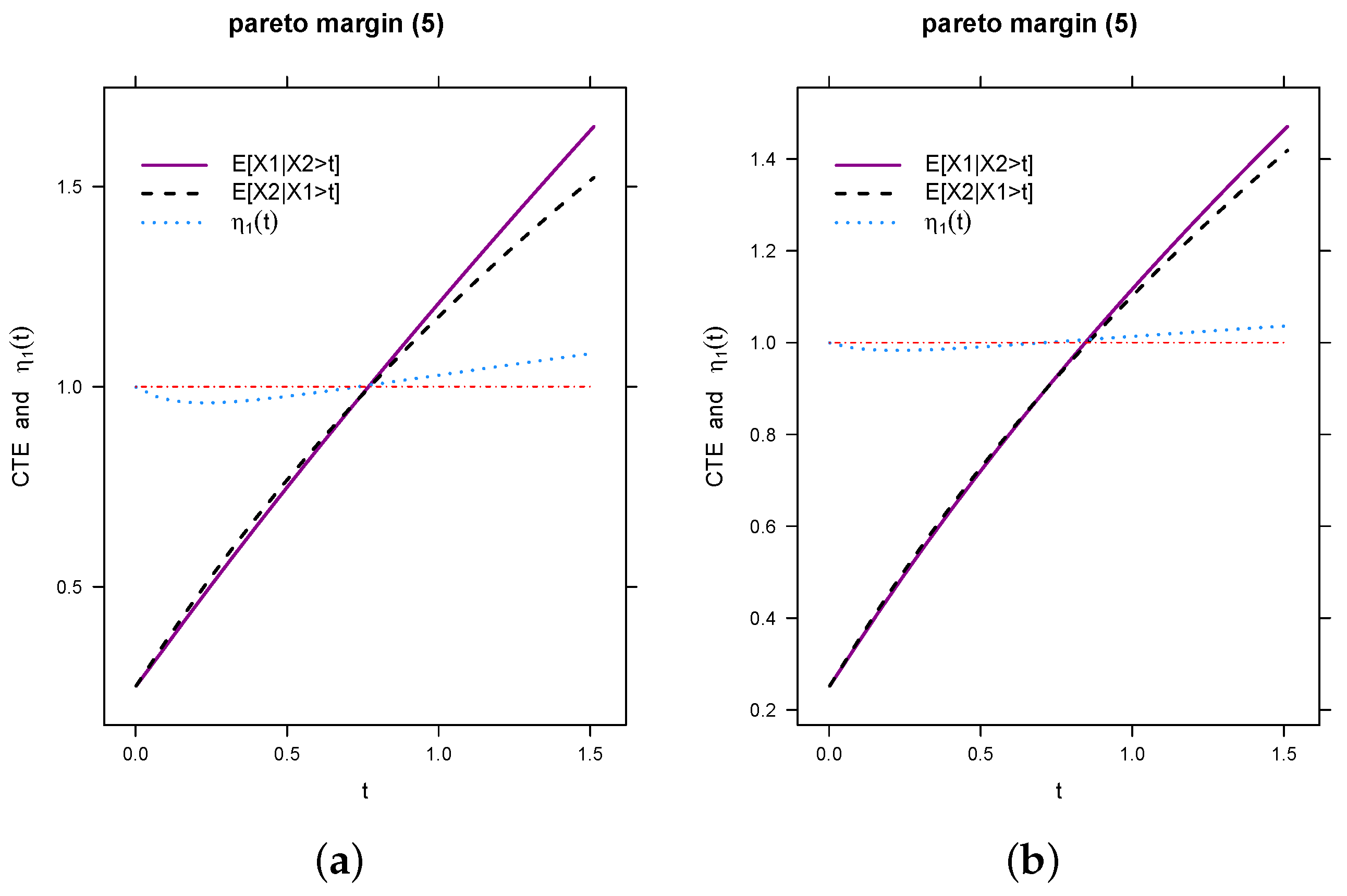
In Figure 1 we present a simulation using the Laplace approximation. In Figure 1a we take and as and , respectively. In Figure 1b we reduce such that its value comes closer to . We do this because if and are the same, we get exchangeability as the result of symmetric copulas. In these two panels we assume and throughout this simulation. The values of and are very high. The main reason is that, if we take lower values, the distance between two conditional expectations are so big that we cannot find any pattern. Apart from that, these Laplace approximation simulations look similar to the simulations when we use Pareto margins and use the definitions of conditional expectations.
Proposition 2.
Let , be a bivariate copula and that and are identically distributed positive random variables with univariate cdf and density function f. Assume and and
For all , and if , , , then,
where , and .
Example 2
(Clayton copula with Weibull marginals). Let be the Clayton copula, such as . Let and follow Weibull distributions with cdf and . Then based on (6), for given , ,
By Proposition 2,
Moreover, , and . Finally before using the result of Proposition 2 we have to show . Here we have,
Both the terms on the right hand side of (14) are always finite. The main reasons are we have and ; which leads us to three possibilities, , and . Let us discuss each of the cases separately. As we have as the first term, it is always finite as . Now, the only thing that matters is the value of γ. When , takes the highest value when . By assumption . So . Under this case we still possibility to have as . Therefore, we need further restrictions on γ. For the bound of is not finite. Furthermore, when , as . Hence, we need to make for any large s. Using the above conditions and Proposition 2 we get
where , and .
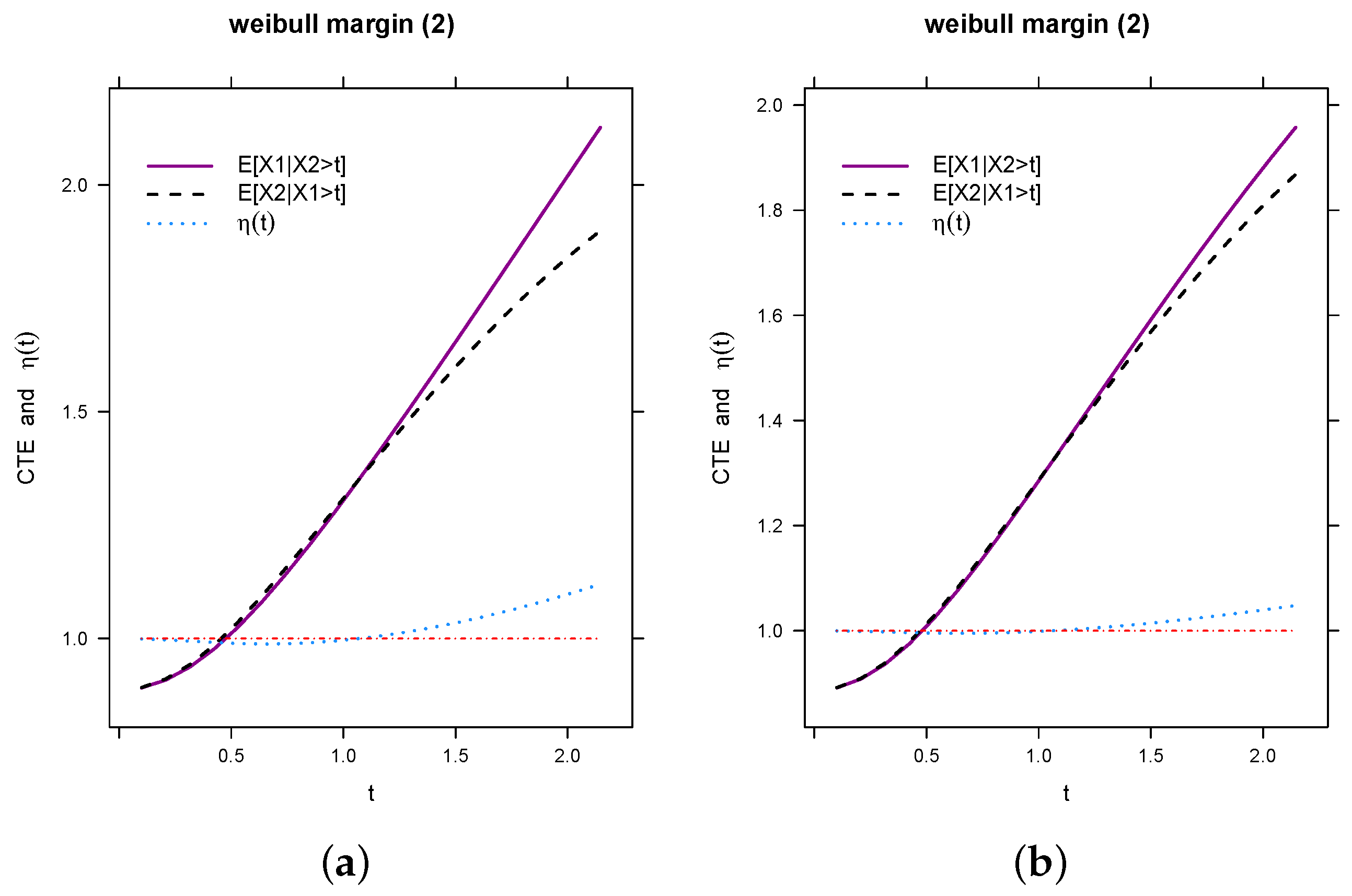
Figure 2a represents a simulation from Watson’s lemma and Figure 2b is the actual integration result. In Figure 2a the dotted black line represents and the purple line represents . The pattern of the movement of the two lines are same but the gap between them is more than in Figure 2b. Hence, we clearly claim that, Watson’s lemma gives more tail non-exchangeability.
Example 3
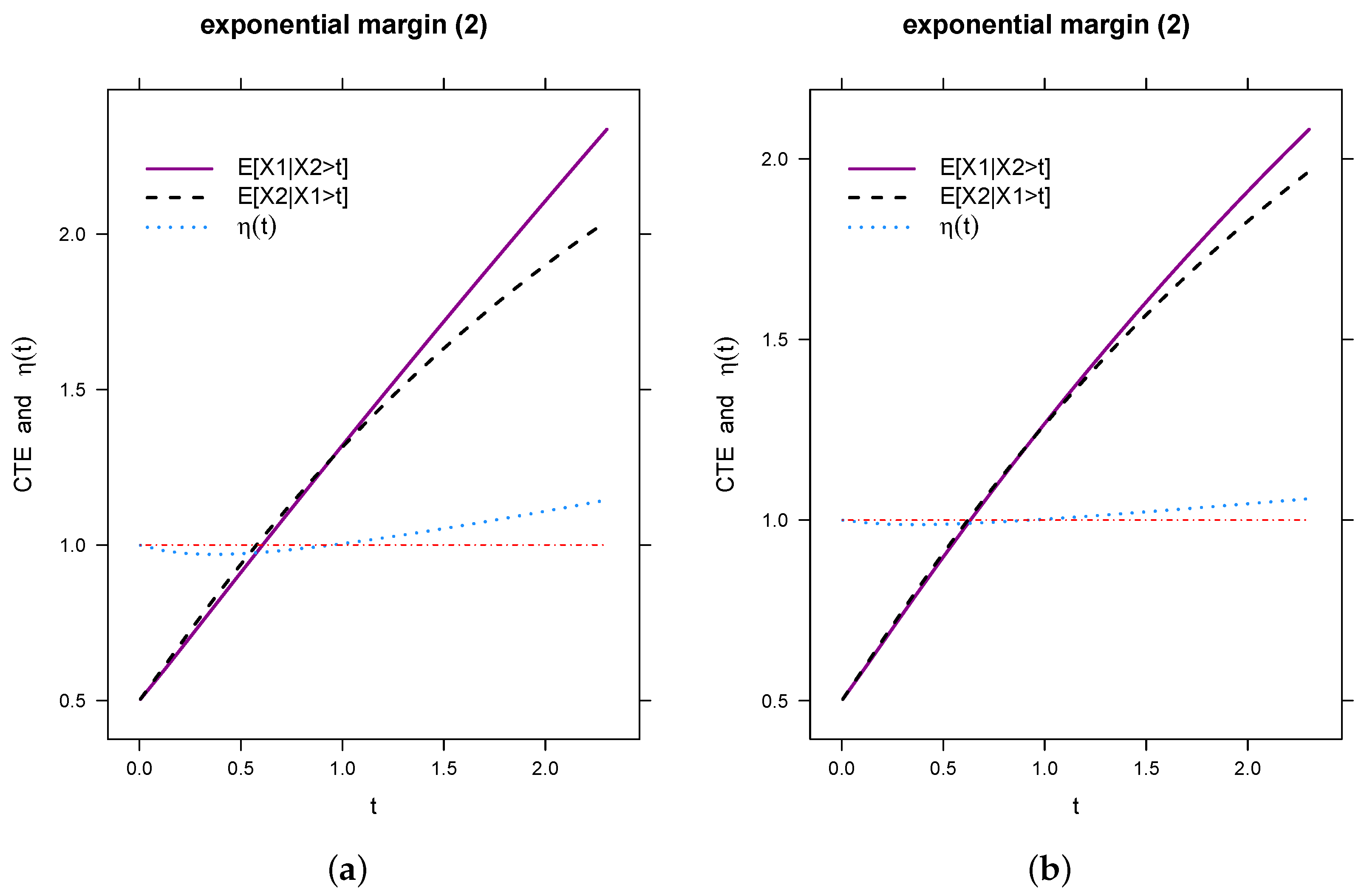
(Clayton copula with Exponential marginals). Like before we have the same Clayton copula but we have exponential marginals. Let and follow Exponential distributions with cdf , for all . For , , and Equation (6) yields
Again, and for all . Moreover,
To satisfy Proposition 2 we need to examine the behavior of around zero. In other words,
for all and . This implies that, the slope of is negative even in the neighborhood of zero. In this case . Furthermore, similar to Weibull case, we can show that, . Proposition 2 implies as , and .
In Figure 3a, we conducted a simulation based on Watson’s lemma. On the right-hand side in Figure 3b, the plot illustrates the results of numerical integration. Upon comparing these two images, it is evident that Watson’s lemma yields nearly identical simulation results. Notably, when employing the KB4 copula with exponential margins, there is a noticeable absence of significant non-exchangeability in the outcomes [19].
3.2. Type II
In this section, our focus is on exploring the non-exchangeability of Type II across three distinct types of univariate marginals. For the Pareto marginal, we employ Laplace’s method, whereas for the Exponential and Weibull cases, we rely on Watson’s lemma to achieve accurate approximations.
Definition 2.
If is a conditional expectation for any given t, then it can be expressed in terms of non-exchangeable copula as , for all t where
with survival functions and , and .
Proposition 3
(Laplace Method). For , let be a bivariate copula, be a conditional bivariate copula, and be identically distributed positive random variables with univariate cdf , and density f. Assume , and write ,
and
For , and if , , , and , for all then,
Example 4
(Clayton copula with Pareto marginals). Let be the Clayton copula, or, . Let be the conditional non-exchangeable Clayton copula with the form,
Let and follow Pareto distributions with cdf , and . Then, based on the combination of and in Proposition 3 implies,
If we carefully look at (18) and combine this result with and in Proposition 3, we observe that, one of the ’s vanishes. As a result, we get only one h function. Therefore, for any . Moreover, since , it can be verified that for any . Also,
which implies that for any given and , there exists such that implies .
For , the root of is
Therefore, we require that to have a well defined root. Clearly, . Consider
where
and
Furthermore,
Again,
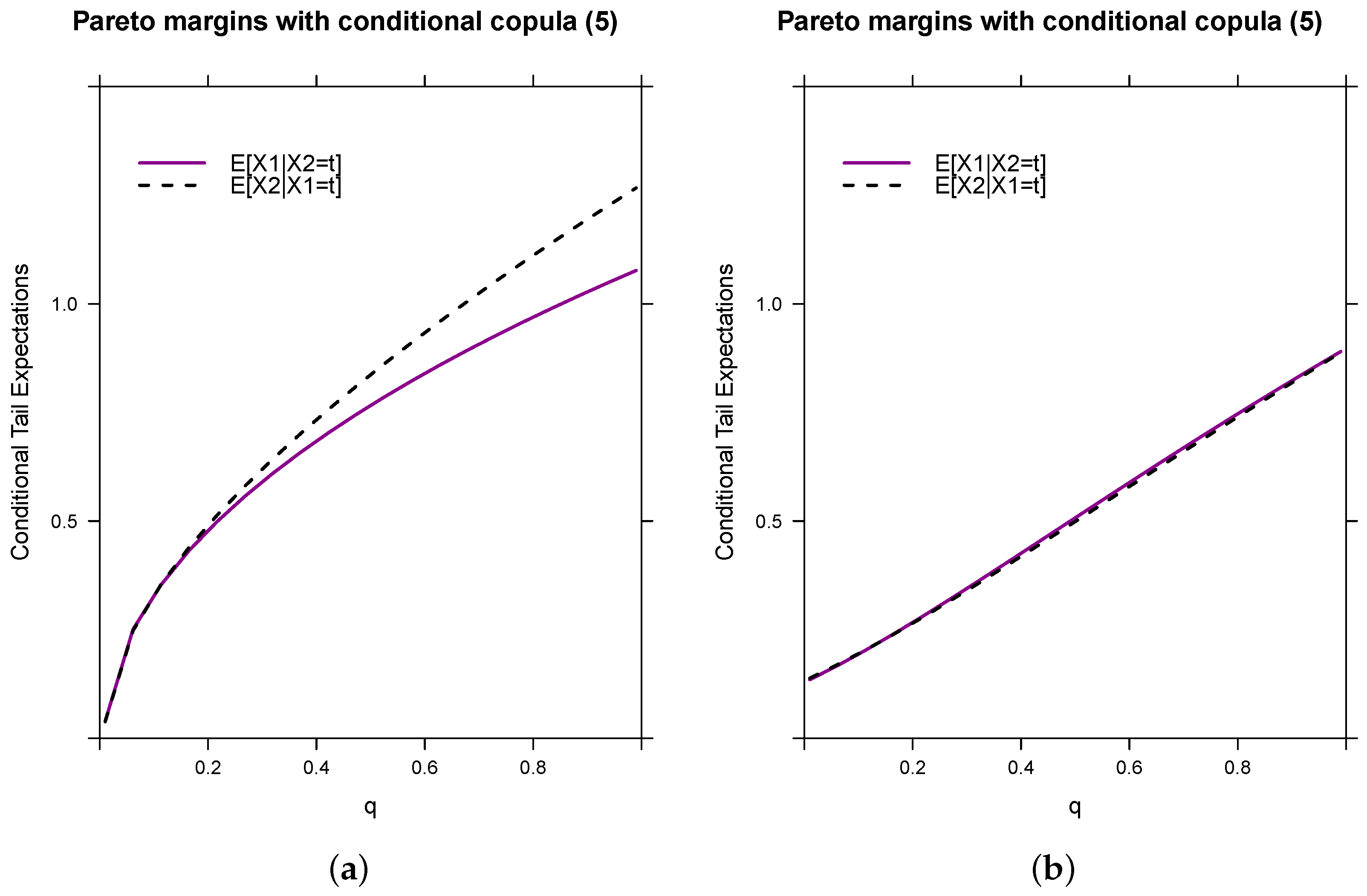
In Figure 4, we juxtapose the simulations using Laplace approximation against the actual conditional tail expectations. In Figure 4a, the simulation results obtained in (22) are utilized, with fixed parameter values of , , , and . The choice of is made to mitigate uneven fluctuations observed at higher and lower values. Despite no discernible pattern in these extreme cases, Figure 4a reveals a lack of significant non-exchangeability around 0, with an increase as we approach the 90th percentile.
On the contrary, Figure 4b shows a relatively subdued presence of non-exchangeability throughout the plot. It is noteworthy that Laplace approximation may tend to overestimate small changes between two tail order conditional expectations at higher quantiles. A closer examination of and reveals their marginal difference. Even when these two parameters are closely aligned, we observe heightened tail non-exchangeability.
Proposition 4.
Let be a bivariate copula, be a conditional bivariate copula. Assume for all , , ,
and
Moreover,
where
and
for all .
Example 5
(Clayton copula with Weibull marginals). Let be the Clayton copula such that . For a conditional non-exchangeable Clayton copula let and follow Weibull marginals with cdf . Then,
By Proposition 4,
In this case, , and . A similar argument like in example 2 implies . Now, Proposition 4 implies
where , , and .
Example 6
(Clayton copula with Exponential marginals). Let be the Clayton copula with conditional non-exchangeable form,
Let and follow Exponential distributions with cdf , for all . Then,
By Equation (28), and for any . Moreover,
Proposition 4 yields
In this example, . A similar analogy like in Example 3 implies
By Proposition 4,
where , , and .
Remark 3.
By examining the h functions presented in Examples 4–6 in relation to Propositions 3 and 4, a notable distinction emerges. In the propositions, the h functions manifest in the combined form of and simultaneously, whereas in the examples, such a duality is absent. This disparity is principally attributed to the dominance of one function (where ) over the other. Consequently, the subordinate function becomes negligible, effectively vanishing in the context of the given examples.
4. Test of Tail Non-Exchangeability
In preceding sections, our analytical exploration has delved into the interplay between univariate marginals and tail non-exchangeability, particularly concerning the Type I and II expectation ratios. Notably, we discovered the utility of this ratio in instances featuring Pareto marginal distributions, thus directing our focus in this section. When endeavoring to construct a statistical test for tail non-exchangeability, the Type I ratio emerges as the more apt choice. This is attributed to the comparative ease in estimating the conditional tail expectation of the form within the framework of the Type I ratio.
Assuming we have observed pairs drawn from the joint distribution of and , a statistical test for bivariate tail non-exchangeability can be formulated when the marginal distributions adhere to a Pareto density. This involves constructing a test based on the estimator for , wherein the empirical version of this estimator is
where , , and indicating the cardinality of the set for . Under the null hypothesis of tail non-exchangeability, the estimator is expected to approximate 1 for large values of t. This characteristic forms the foundation for an approximate statistical test. Given that the numerator and denominator of involve essential sample means, establishing asymptotic normality becomes straightforward.
Proposition 5.
Let and for with unbounded support on for fixed . If and are exchangeable then
where , and
such that, , , and .
Proof.
See in the Appendix A. □
To apply Proposition 5 in constructing a statistical test, one can set a fixed value for t and compare with a normal rejection region. Here, represents an estimation of , derived either from its empirical form or an alternative method, such as the bootstrap. In the case of a bootstrap-based estimator, both parametric and nonparametric bootstrap techniques can be readily adjusted [6].
For the parametric bootstrap, resampling from the joint distribution under the assumption of exchangeability can be accomplished by initially simulating using a fitted copula. Subsequently, transformations and for are applied [6]. Here, denotes the estimated common marginal distribution based on the combined observed data from each margin.
For the nonparametric bootstrap, generating a resample under the assumption of exchangeability involves simulating for and . In this expression, is a simulated observation from the empirical distribution of , is a simulated observation from the empirical distribution of , and Q is a Bernoulli random variable with a success probability of , independent of and [6]. It is important to note that is also independent of .
Given the emphasis on tail exchangeability, it is reasonable to choose a large value for t. Nevertheless, the selection of t should be carefully weighed against the availability of data beyond t, as this factor influences the standard error of . The reliance on a specific value of t in the methodology is unattractive due to the potential for test results to vary based on this choice. As an alternative approach, we propose aggregating the test over a range of t values and using the maximum difference as the test statistic.
In particular, let and , where , represent two estimated marginal quantiles determined by observed data. Compute for , where forms a grid of values. The test statistic for assessing the null hypothesis of exchangeability is then expressed as
The rejection region for this test statistic can be calculated using the bootstrap method.
The effectiveness of the weak convergence, as outlined in Proposition 5, may necessitate considerably large sample sizes. This stems from the fact that the effective sample size diminishes, given that only data in the upper tail is utilized in computing . Moreover, the nature of being a ratio implies that skewness may persist in the sampling distribution until sample sizes reach substantial magnitudes. These observations are validated by a small-scale empirical study conducted on a computer.
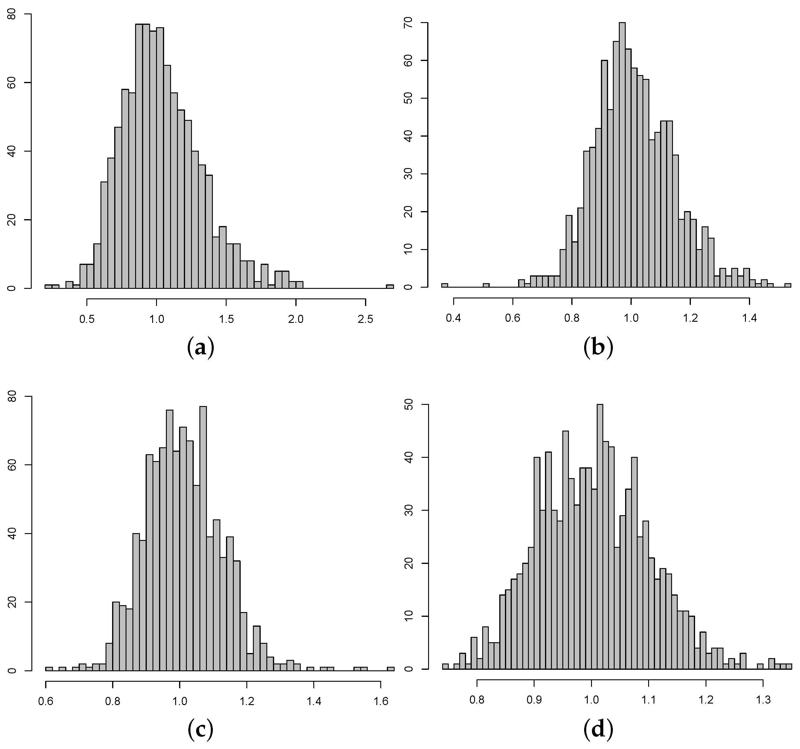
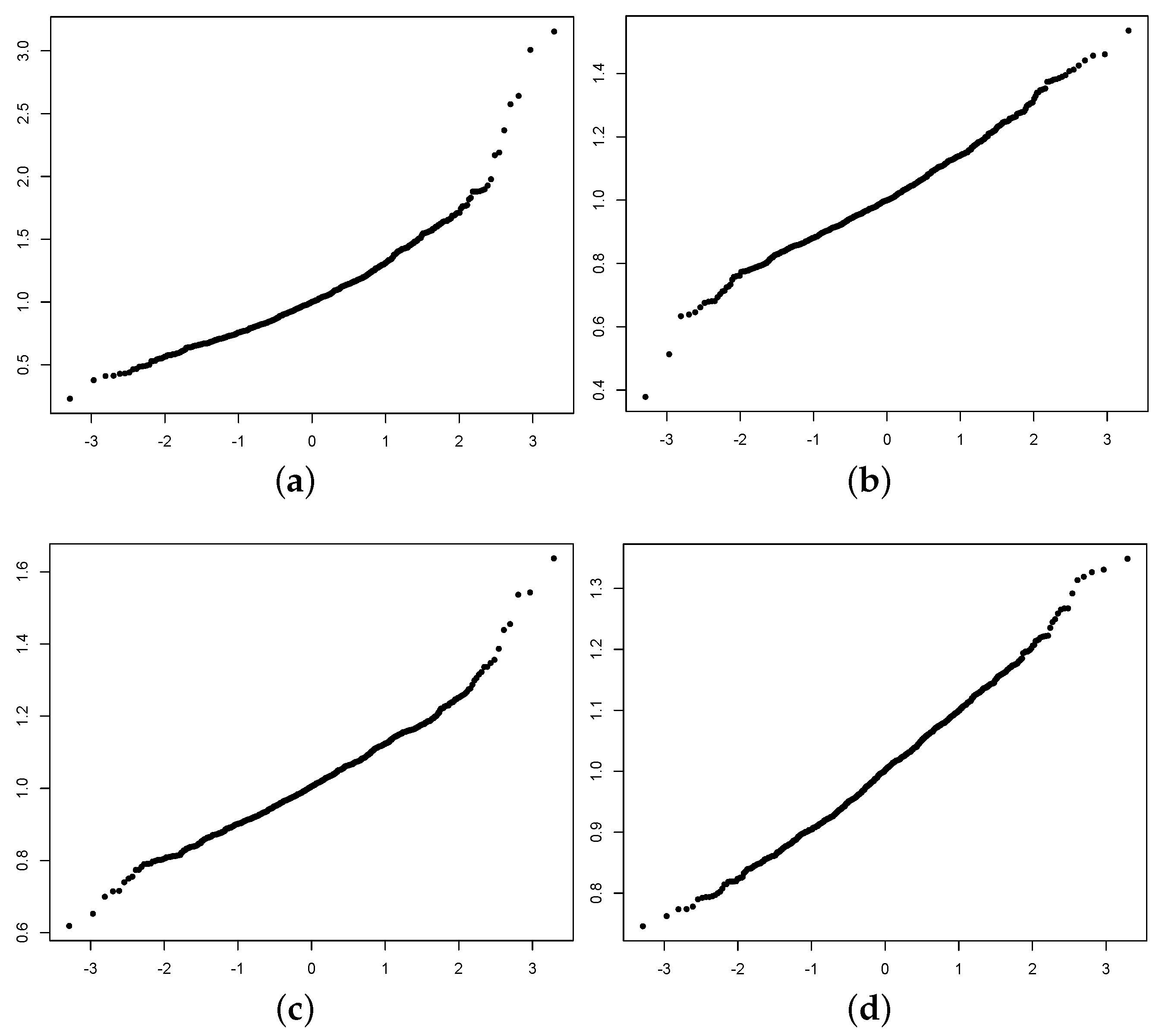
In this study, we generated 1000 samples of sizes , 500, 750, and 1000 from an exchangeable joint distribution with Pareto marginals (shape parameter = 3, scale parameter = 1), exponential marginals (rate = 2), and Weibull marginals (shape parameter = 2). We computed for each simulated sample, where t was chosen to be the 0.75 quantile of the marginal distribution. The results of this investigation underscore the need for ample sample sizes to observe the intended convergence.
Figure 5 and Figure 6 present histograms and normal quantile plots corresponding to each sample size. These visual representations not only illustrate the occurrence of convergence to a normal distribution but also underscore the relatively gradual pace of this convergence. These findings reinforce the notion of resorting to the bootstrap method in practical scenarios, emphasizing its utility in situations where convergence is not swiftly achieved.
5. Real Data Analysis
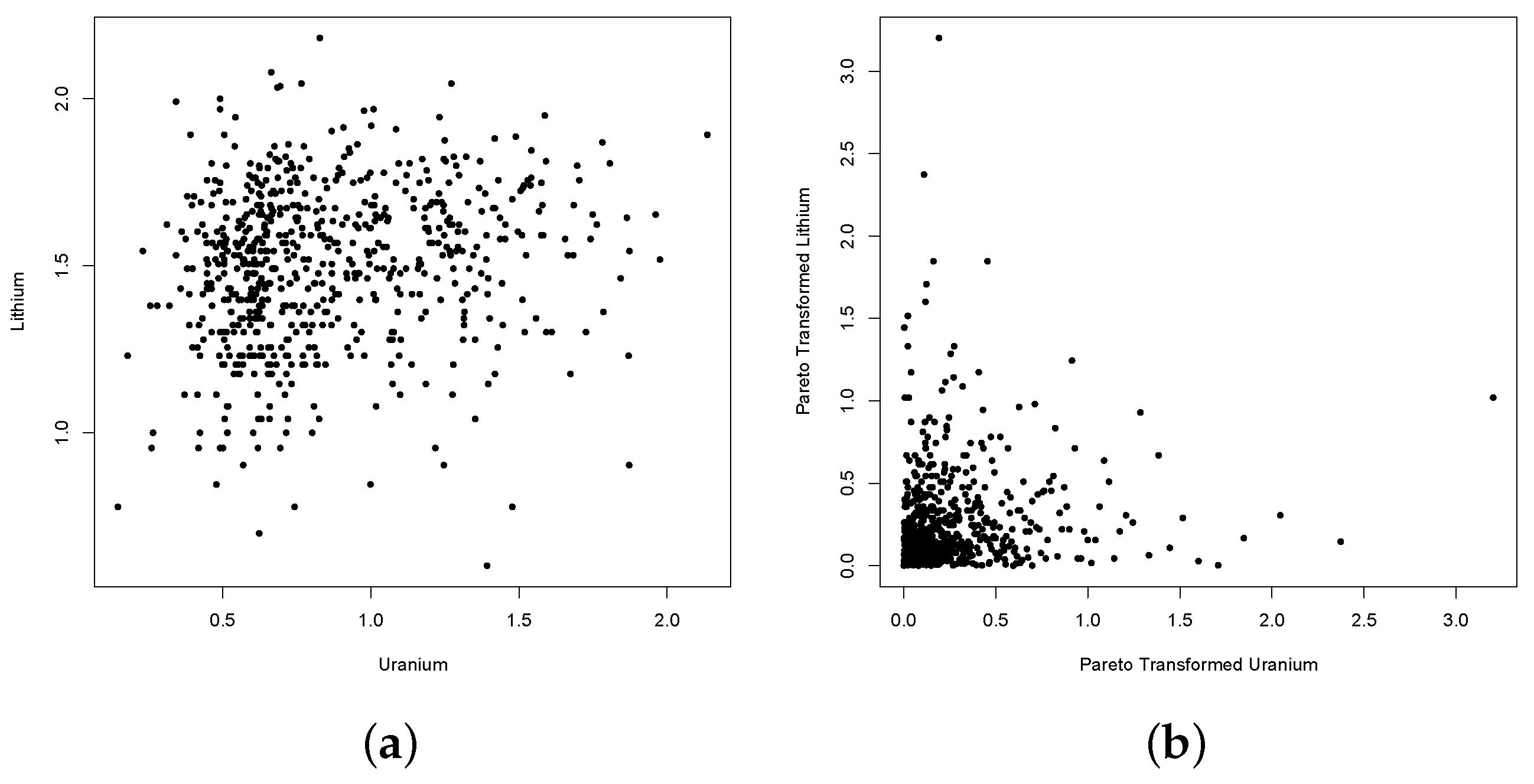
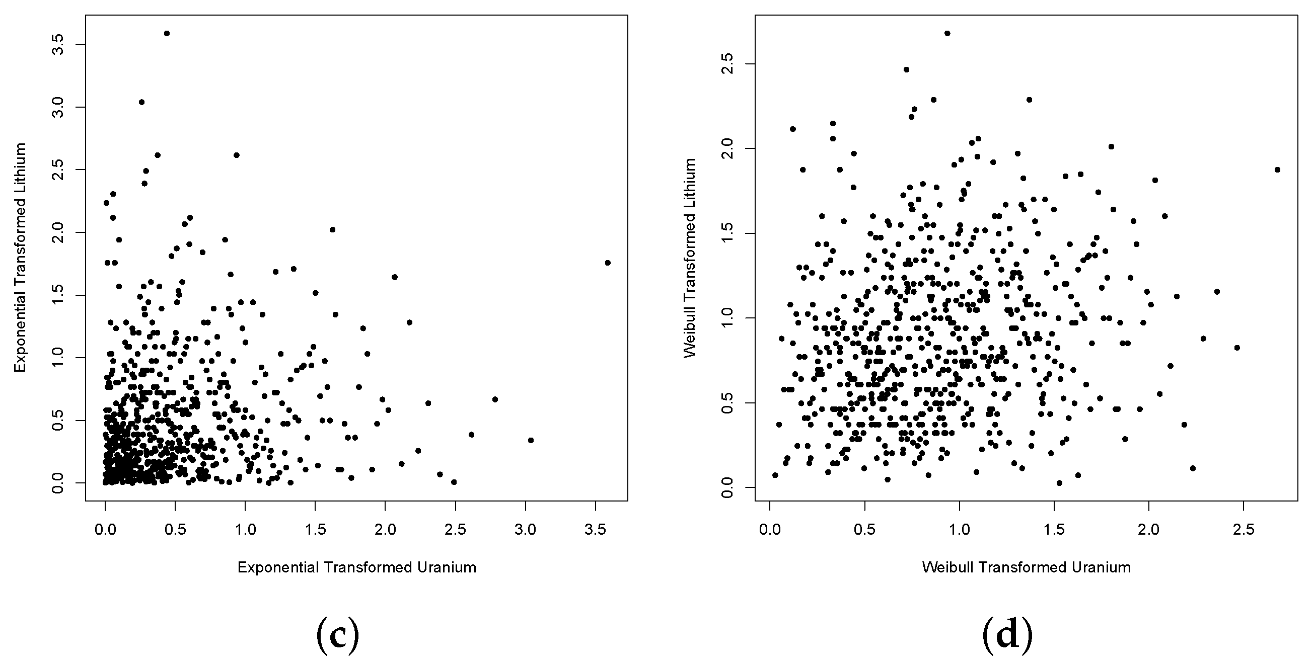
To illustrate the practical application of this test, we leverage the dataset from Cook et al. (1986) [20], which encompasses the observed log-concentration values of seven chemical elements in 655 water samples collected near Grand Junction, Colorado. Our focus centers on exploring the joint distributions of Uranium and Lithium, as well as Uranium and Titanium. The original data sets are visually depicted in Figure 7 and Figure 8. Recognizing that the original data likely do not share identical marginal distributions, and aiming for demonstrative clarity, we undertake three distinct transformations for each dataset. Initially, we employ a joint rank transformation on the data, scaling the results to the unit interval. This preprocessing step sets the stage for a nuanced analysis of the interplay between Uranium and the selected chemical elements. That is, we computed () for where
where is the rank of relative to for and . To facilitate a meaningful comparison, we proceeded by transforming the previously scaled ranks to achieve identical marginal distributions through the probability integral transformation. In this endeavor, we explored three distinct marginal models: a Pareto distribution characterized by a shape parameter of 5, an exponential distribution with a rate set at 2, and a Weibull distribution featuring a shape parameter of 2. The outcomes of these transformations are visually depicted in Figure 7 and Figure 8, showcasing the resulting joint distributions for the transformed data.
The assessment of tail exchangeability was conducted for each case through the bootstrap methodology detailed earlier. The outcomes of these calculations are visually presented in Figure 9, Figure 10, Figure 11, Figure 12, Figure 13 and Figure 14. In the left panel of each figure, the values of are depicted for a range of t values corresponding to the interval between the 75th and 95th percentiles of the observed marginal distribution of the combined data. The grey lines represent the values computed across 500 nonparametric bootstrap resamples.
Moving to the right panel in each figure, a histogram displays the distribution of test statistic values computed for each of the 500 resamples. If present, a vertical line indicates the observed value of from the sample. The bootstrap-generated p-values, signaling the test of the null hypothesis of Type I exchangeability, are detailed in Table 1. From the estimated p-values, a clear pattern emerges: there is substantial evidence opposing exchangeability for the joint distributions of Uranium and Titanium, whereas there is limited evidence against exchangeability for the joint distributions of Uranium and Lithium.
Given the results outlined in the sections above, it may seem surprising at first to observe notable outcomes in the exponential and Weibull scenarios. However, this outcome appears to be linked to the nature of the test statistic . The emphasis of on the relative ranks of the two observed marginal distributions, rather than the gaps between the actual values, explains this unexpected pattern. This inclination is evident in the consistent behavior observed in the curves of across different marginal distributions. The impact of relative ranks, rather than absolute values, seems to contribute to the observed significance in these specific cases.
6. Discussion
Throughout this manuscript, our primary focus is on quantifying the extent of tail non-exchangeability. We commence by introducing metrics specifically crafted to measure the strength of tail non-exchangeability, leveraging conditional tail expectations. Subsequent to this, we present theoretical outcomes for non-exchangeable bivariate copulas generated using Khoudraji’s device, in conjunction with three distinct types of univariate marginals. Our findings underscore the heightened significance of tail non-exchangeability when Pareto marginals are chosen. Consequently, we advocate for the transformation of each marginal distribution to adhere to a Pareto distribution. In the pursuit of detecting tail non-exchangeability, we put forward a graphical tool grounded in theoretical insights, accompanied by a statistical test. We have used the R package CopulaModel to perform the copula related simulations and boot to do the empirical studies.
The proposed method in this study introduces a test statistic derived from the ratio of conditional tail expectations to effectively identify instances of tail non-exchangeability. It acknowledges the challenge of establishing limiting properties empirically, especially when concentrating on extreme values that involve fewer data points, leading to a potential loss of information from the entire dataset.
To mitigate this limitation, the study adopts a strategy involving a series of upper sets of data when testing non-exchangeability. The asymptotic normality of the proposed test statistic has been rigorously demonstrated under mild conditions as the sample size tends towards infinity. For practical applications with unknown variability, the paper suggests the use of bootstrap methods.
Focusing specifically on non-exchangeability in the context of positive dependence, the methodology can be extended to bivariate copulas exhibiting tail negative dependence. However, it is worth noting that the approach is tailored for bivariate cases. To apply it to cases with tail negative dependence, one can easily transform one of the marginals to ensure positive dependence, facilitating the direct application of the proposed method. Addressing tail non-exchangeability in multivariate scenarios requires employing the approach for all pairwise bivariate marginals. Nevertheless, it is crucial to highlight that pairwise exchangeability does not necessarily imply mutual exchangeability. As a result, further research is warranted to explore and understand the implications of mutual exchangeability in multivariate cases.
This form of tail non-exchangeability holds significance in the realm of time series analysis, particularly when assessing how two random variables evolve over time. Such occurrences are evident when examining the exchangeability of market shares between two distinct companies operating in the same industry. If these shares exhibit exchangeability, it becomes possible to predict future share prices for one company based on the knowledge of the other. Looking ahead, we can explore the presence of tail exchangeability among different soccer positions across various teams [21]. For instance, our method can be applied to test the exchangeability of goal dynamics between two strikers from different clubs in the European Football League. If these dynamics prove to be exchangeable, it implies that a club can seamlessly replace one striker with another once the first striker’s contract expires. A similar analysis can be conducted for different batting positions in cricket matches involving various teams.
In the context of infectious disease modeling, the widely used susceptibility-infection-recovery (SIR) framework comes into play [22,23]. Our method allows for testing exchangeability by examining different SIR datasets between two regions. If exchangeability is established, it suggests that a specific vaccination strategy could lead to recovery from infectious diseases in those regions. This versatile approach extends its applicability to diverse fields, showcasing its potential for extracting meaningful insights from various types of data.
These tests of non-exchangeability serve a crucial role during financial upheavals like the Great Depression (1930–1937), the Oil crisis (1968–1970 to 1972–1978), Black Monday (1987), and the series of crises from Asia to the millennium leading up to the Dot-Com crisis (1995–2003). It is widely acknowledged that during crises, losses tend to escalate dramatically, leading to a heightened correlation among extreme losses and, consequently, an uptick in the co-movement of extreme gains. This phenomenon serves as a form of compensation for investors who face substantial downside risks across various sectors [1]. In simpler terms, when significant losses occur more frequently, one can anticipate a corresponding increase in significant gains happening simultaneously. However, in contrast, the 2007–2009 financial crisis stands out due to a temporary spike in tail asymmetries, contrasting with the overall declining trend in tail asymmetries since the mid-1990s. Some may argue that only losses exhibiting tail dependence were impacted, while the tail dependence between gains remained unaffected [1]. This highlights the particularly devastating nature of the subprime crisis, as investors did not encounter as much potential for extreme upside gains. In the literature of econometrics and time series, the main focus of risk management is on Value-at-Risk (VaR), and other measures designed to estimate the probability of large losses, leading to a demand for flexible models of the dependence between sources of risk [24]. Therefore, the non-exchangeable structures might exist.
In clinical research, when censoring occurs due to competing risks or patient withdrawal, there’s always a concern regarding the accuracy of treatment effect estimates derived under the assumption of independent censoring [25]. Since identifying dependent censoring requires additional information, the most we can do is conduct a sensitivity analysis to evaluate how parameter estimates change under varying assumptions regarding the relationship between failure and censoring. Such an analysis proves particularly valuable when insights into this relationship are available through literature reviews or expert opinions [25]. In regression analysis, the repercussions of mistakenly assuming independent censoring on parameter estimates are unclear. Neither the direction nor the extent of potential bias can be easily anticipated. It is assumed that the joint distribution of failure and censoring times is a function of their distributions, with this function represented as a copula function. Under this assumption, one can examine dependencies at the tails to assess the non-exchangeability.
Funding
This research received no external funding.
Institutional Review Board Statement
Not applicable.
Informed Consent Statement
Not applicable.
Data Availability Statement
The dataset from Cook et al. (1986) [20] has been used.
Conflicts of Interest
The author declares no conflict of interest.
Appendix A
Proof of Proposition 1.
Since , changing of variables yields, . For , the above condition in (A1) yields,
Let . Therefore, . Substituting this condition in (A2) yields,
By Laplace’s method,
which completes the proof. □
Proof of Proposition 2.
To prove this proposition we are using Theorem 36 of Breitung (2006) [26] (p. 48). Since is a real valued function on the semi-infinite interval and in an interval with , this function is continuously differentiable and , with .
If and , following Theorem 36 of Breitung (2006) [26] implies Now, if we assume , then
This version of Watson’s lemma requires to be constant, which is possible only if
is a constant. In other words, if is a constant. Thus,
or, .
Let there be a real and continuous function such that with . More specifically in our case we have, . Thus, when . As we assume then
for all , where and . This completes the proof. □
Proof of Proposition 3.
Since , changing of variables yields, . Above condition with (A5) implies,
Let , and thus . This condition with (A6) yields,
where and . Now we have two separate integrations consist of (with ) functions each of which behaves similarly like in Proposition 1. Here . Thus, Laplace Method implies, for all . Finally, the conditional expectation becomes,
□
Proof of Proposition 4.
We are using Theorem 36 of [26] (p. 48). Since and are real valued functions on , and , for all , with with
where .
For and we have and for all . Moreover, , and . Assume . Then and, and . Furthermore,
such that , and
such that which are constants at and . Therefore, or, . Similarly, .
Let there be another real and continuous function such that, with and . Moreover, , . Hence, implies , where .
Now,
where , ,
and
for all . □
Proof of Proposition 5.
Consider a set of bivariate random vectors for , where for and . This corresponds to a sequence of independent and identically distributed random vectors such that
where and . The covariance matrix of is
where , and . Under the null hypothesis of exchangeability, the multivariate central limit theorem implies that as . To obtain the weak convergence described in Proposition 5 we firstly apply the delta method (Theorem 3.1 of van der Vaat (2000) [27]) to obtain
where . The asymptotic normality of then follows from Slutsky’s theorem and the fact that as . □
References
- Bormann, C.; Schienle, M. Detecting structural differences in tail dependence of financial time series. J. Bus. Econ. Stat. 2020, 38, 380–392. [Google Scholar] [CrossRef]
- Li, F. Identifying asymmetric comovements of international stock market returns. J. Financ. Econom. 2014, 12, 507–543. [Google Scholar] [CrossRef]
- Longin, F.; Solnik, B. Extreme correlation of international equity markets. J. Financ. 2001, 56, 649–676. [Google Scholar] [CrossRef]
- Embrechts, P. Linear correlation and evt: Properties and caveats. J. Financ. Econom. 2009, 7, 30–39. [Google Scholar] [CrossRef]
- Koike, T.; Kato, S.; Hofert, M. Measuring non-exchangeable tail dependence using tail copulas. ASTIN Bull. J. IAA 2023, 53, 466–487. [Google Scholar] [CrossRef]
- Hua, L.; Polansky, A.; Pramanik, P. Assessing bivariate tail non-exchangeable dependence. Stat. Probab. Lett. 2019, 155, 108556. [Google Scholar] [CrossRef]
- Furman, E.; Su, J.; Zitikis, R. Paths and indices of maximal tail dependence. ASTIN Bull. 2015, 45, 661–678. [Google Scholar] [CrossRef]
- Hua, L.; Joe, H. Multivariate dependence modeling based on comonotonic factors. J. Multivar. Anal. 2017; in press. [Google Scholar]
- Khoudraji, A. Contributions à l’Étude des Copules et à la Modélisation de Valeurs Extrêmes Bivariées. Ph.D. Thesis, Université Laval Québec, Quebec, QC, Canada, 1996. [Google Scholar]
- Hua, L.; Joe, H. Tail order and intermediate tail dependence of multivariate copulas. J. Multivar. Anal. 2011, 102, 1454–1471. [Google Scholar] [CrossRef]
- Garcia, R.; Tsafack, G. Dependence structure and extreme comovements in international equity and bond markets. J. Bank. Financ. 2011, 35, 1954–1970. [Google Scholar] [CrossRef]
- Sibuya, M. Bivariate extreme statistics. Ann. Inst. Stat. Math. 1960, 11, 195–210. [Google Scholar] [CrossRef]
- Genest, C.; Jaworski, P. On the class of bivariate archimax copulas under constraints. Fuzzy Sets Syst. 2021, 415, 37–53. [Google Scholar] [CrossRef]
- Hua, L.; Joe, H. Strength of tail dependence based on conditional tail expectation. J. Multivar. Anal. 2014, 123, 143–159. [Google Scholar] [CrossRef]
- Bernard, C.; Czado, C. Conditional quantiles and tail dependence. J. Multivar. Anal. 2015, 138, 104–126. [Google Scholar] [CrossRef]
- Genest, C.; Kojadinovic, I.; Nešlehová, J.; Yan, J. A goodness-of-fit test for bivariate extreme-value copulas. Bernoulli 2011, 17, 253–275. [Google Scholar] [CrossRef]
- Genest, C.; Nešlehová, J.; Quessy, J.-F. Tests of symmetry for bivariate copulas. Ann. Inst. Stat. Math. 2012, 64, 811–834. [Google Scholar] [CrossRef]
- Genest, C.; Ghoudi, K.; Rivest, L.-P. Understanding relationships using copulas. N. Am. Actuar. J. 1998, 2, 143–149. [Google Scholar] [CrossRef]
- Pramanik, P. Tail Non-Exchangeability. M.S. Thesis, Northern Illinois University, DeKalb, IL, USA, 2016. [Google Scholar]
- Cook, R.D.; Johnson, M.E. Generalized burr-pareto-logistic distributions with applications to a uranium exploration data set. Technometrics 1986, 28, 123–131. [Google Scholar] [CrossRef]
- Pramanik, P.; Polansky, A.M. Scoring a goal optimally in a soccer game under liouville-like quantum gravity action. In Operations Research Forum; Springer: Berlin/Heidelberg, Germany, 2023; Volume 4, p. 66. [Google Scholar]
- Pramanik, P. Path integral control of a stochastic multi-risk sir pandemic model. Theory Biosci. 2023, 142, 107–142. [Google Scholar] [CrossRef] [PubMed]
- Pramanik, P. Optimal lock-down intensity: A stochastic pandemic control approach of path integral. Comput. Math. Biophys. 2023, 11, 20230110. [Google Scholar] [CrossRef]
- Patton, A. A review of copula models for economic time series. J. Multivar. Anal. 2012, 110, 4–18. [Google Scholar] [CrossRef]
- Huang, X.; Zhang, N. Regression survival analysis with an assumed copula for dependent censoring: A sensitivity analysis approach. Biometrics 2008, 64, 1090–1099. [Google Scholar] [CrossRef] [PubMed]
- Breitung, K.W. Asymptotic Approximations for Probability Integrals; Springer: Berlin/Heidelberg, Germany, 2006. [Google Scholar]
- Der Vaart, A.W.V. Asymptotic Statistics; Cambridge University Press: Cambridge, UK, 2000; Volume 3. [Google Scholar]
Figure 1.
Comparison of and when and are different, using Laplace Approximation. (a) 0.97, 0.85, 10. (b) 0.90, 0.85, 10.
Figure 1.
Comparison of and when and are different, using Laplace Approximation. (a) 0.97, 0.85, 10. (b) 0.90, 0.85, 10.

Figure 2.
Comparison of , , and for Weibull margins when and are different, , , and t takes values from the 1st percentile to the 99th percentile. (a) 0.97, 0.85. (b) 0.90, 0.85.
Figure 2.
Comparison of , , and for Weibull margins when and are different, , , and t takes values from the 1st percentile to the 99th percentile. (a) 0.97, 0.85. (b) 0.90, 0.85.

Figure 3.
Comparison of , , and for exponential margins when and are different, , , and t takes values from the 1st percentile to the 99th percentile. (a) , . (b) , .
Figure 3.
Comparison of , , and for exponential margins when and are different, , , and t takes values from the 1st percentile to the 99th percentile. (a) , . (b) , .

Figure 4.
Comparison Between Laplace Approximation and the Actual Conditional Tail Expectations when and are Different. (a) 0.85, 0.90, 5 and . (b) 0.85, 0.90, 5 and .
Figure 4.
Comparison Between Laplace Approximation and the Actual Conditional Tail Expectations when and are Different. (a) 0.85, 0.90, 5 and . (b) 0.85, 0.90, 5 and .

Figure 5.
Histograms of the 1000 simulated realizations of from the empirical study where the marginal distributions are Pareto. (a) . (b) . (c) . (d) .
Figure 5.
Histograms of the 1000 simulated realizations of from the empirical study where the marginal distributions are Pareto. (a) . (b) . (c) . (d) .

Figure 6.
Normal quantile plots of the 1000 simulated realizations of from the empirical study where the marginal distributions are Pareto. (a) . (b) . (c) . (d) .
Figure 6.
Normal quantile plots of the 1000 simulated realizations of from the empirical study where the marginal distributions are Pareto. (a) . (b) . (c) . (d) .

Figure 7.
Scatter plots of the observed joint distribution between Uranium and Lithium for the original and transformed marginal data. Panel (a) represents the scatterplot from raw data. Panel (b–d) are the scatterplots after Pareto, exponential and Weibull transformations respectively.
Figure 7.
Scatter plots of the observed joint distribution between Uranium and Lithium for the original and transformed marginal data. Panel (a) represents the scatterplot from raw data. Panel (b–d) are the scatterplots after Pareto, exponential and Weibull transformations respectively.


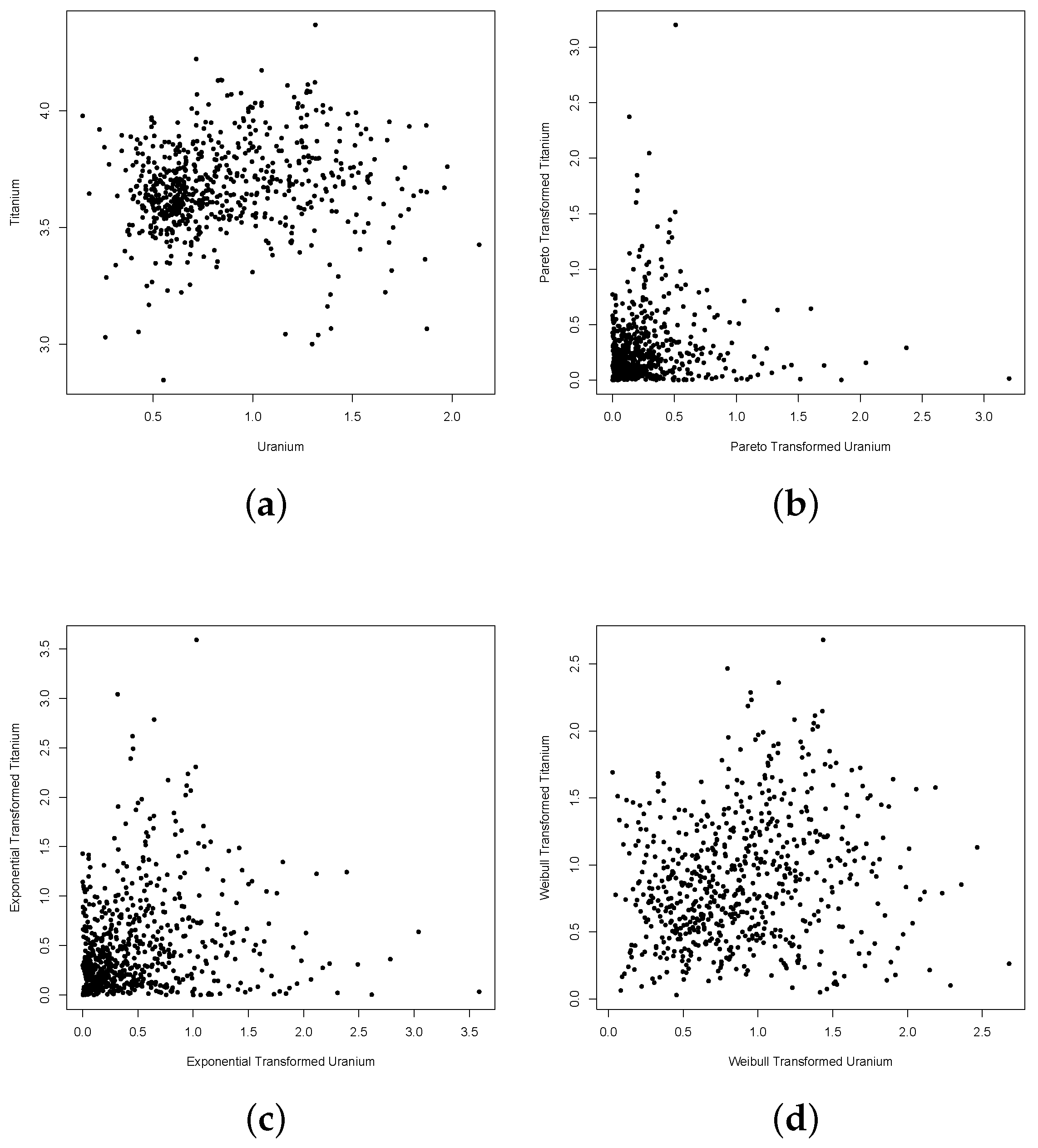
Figure 8.
Scatter plots of the observed joint distribution between Uranium and Titanium for the original and transformed marginal data. Panel (a) represents the scatterplot from raw data. Panel (b–d) are the scatterplots after Pareto, exponential and Weibull transformations respectively.
Figure 8.
Scatter plots of the observed joint distribution between Uranium and Titanium for the original and transformed marginal data. Panel (a) represents the scatterplot from raw data. Panel (b–d) are the scatterplots after Pareto, exponential and Weibull transformations respectively.

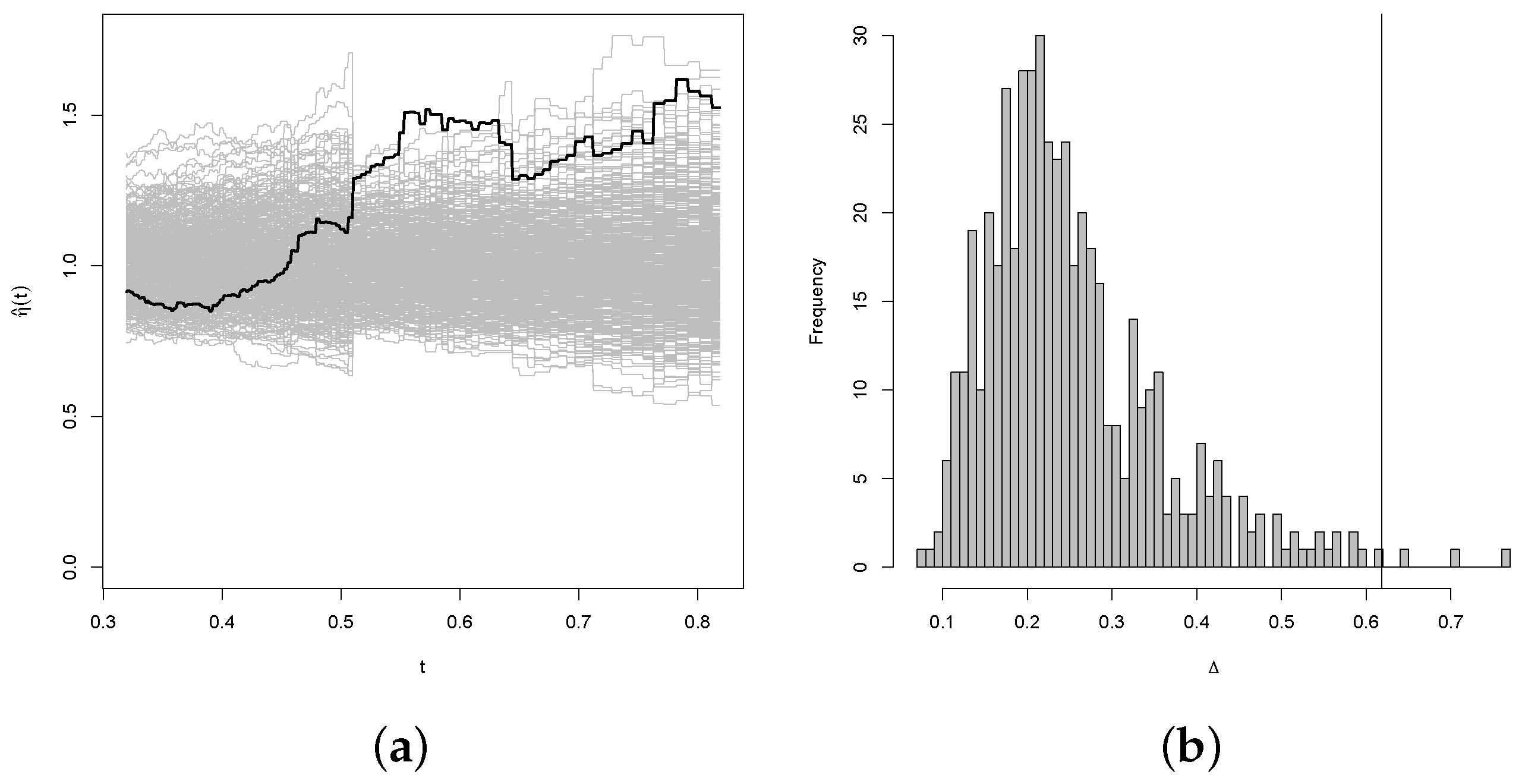
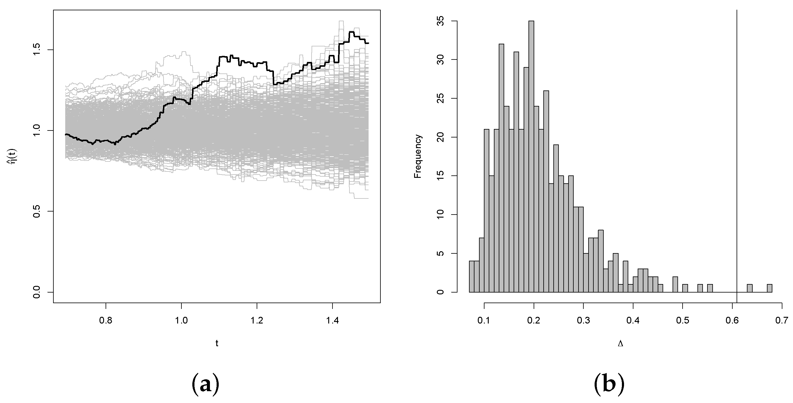
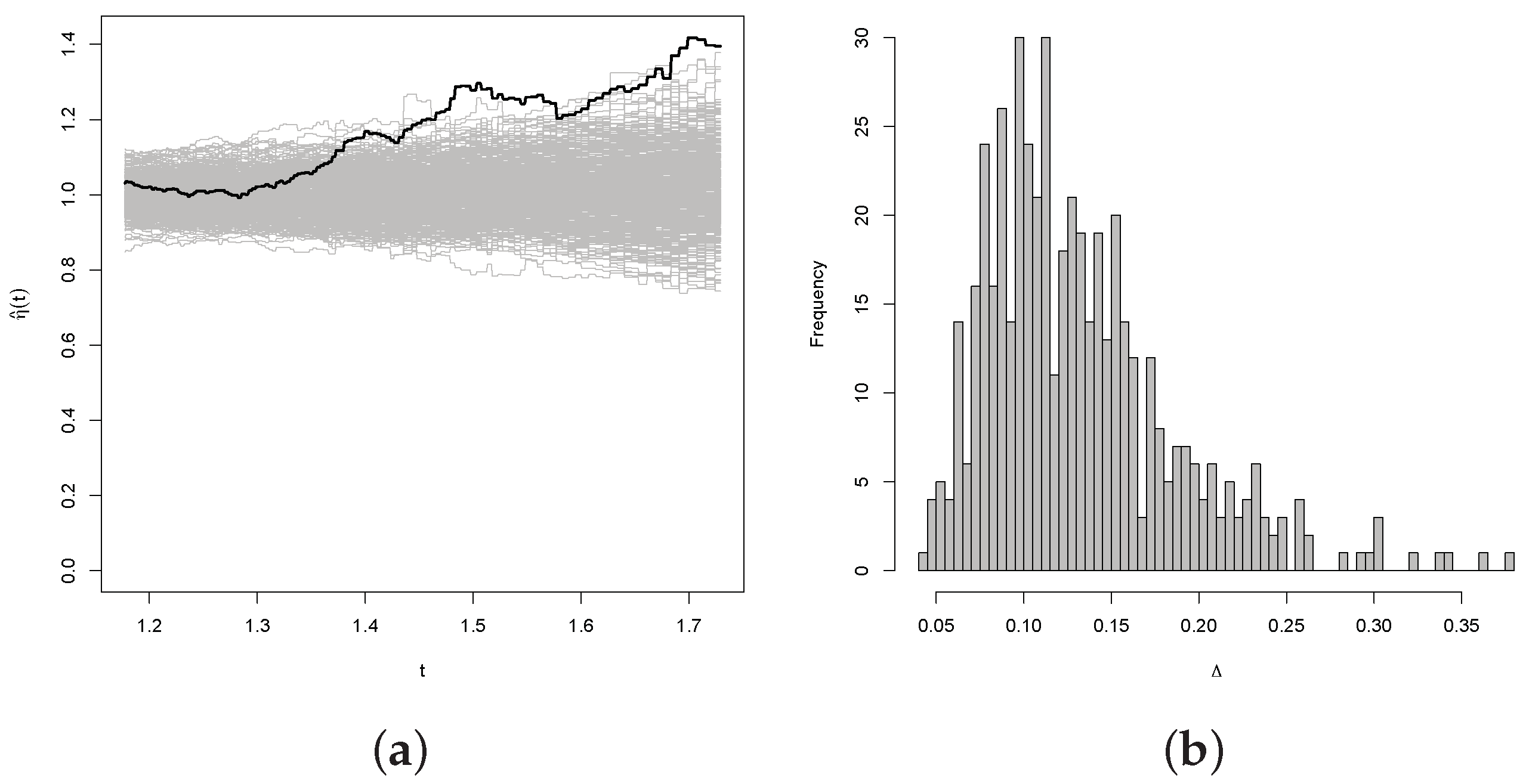
Figure 9.
Results of the bootstrap test of the null hypothesis of exchangeability for the joint distribution of Uranium and Lithium with Pareto marginal distributions. The thick line in panel (a) represents the expectation of the simulation. Panel (b) represents the histogram of the simulation.
Figure 9.
Results of the bootstrap test of the null hypothesis of exchangeability for the joint distribution of Uranium and Lithium with Pareto marginal distributions. The thick line in panel (a) represents the expectation of the simulation. Panel (b) represents the histogram of the simulation.

Figure 10.
Results of the bootstrap test of the null hypothesis of exchangeability for the joint distribution of Uranium and Lithium with exponential marginal distributions. The thick line in panel (a) represents the expectation of the simulation. Panel (b) represents the histogram of the simulation.

Figure 11.
Results of the bootstrap test of the null hypothesis of exchangeability for the joint distribution of Uranium and Lithium with Weibull marginal distributions. The thick line in panel (a) represents the expectation of the simulation. Panel (b) represents the histogram of the simulation.
Figure 11.
Results of the bootstrap test of the null hypothesis of exchangeability for the joint distribution of Uranium and Lithium with Weibull marginal distributions. The thick line in panel (a) represents the expectation of the simulation. Panel (b) represents the histogram of the simulation.

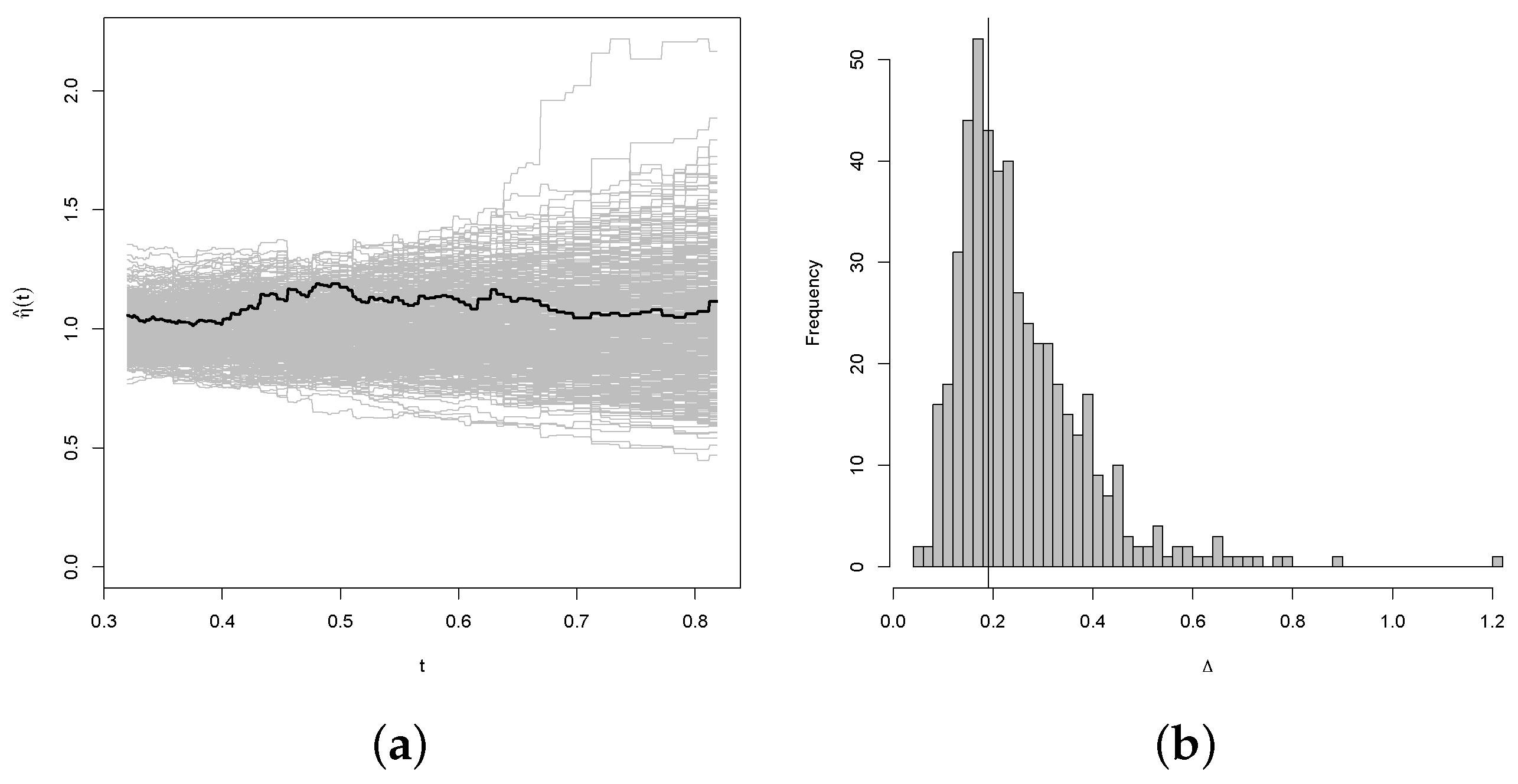
Figure 12.
Results of the bootstrap test of the null hypothesis of exchangeability for the joint distribution of Uranium and Titanium with Pareto marginal distributions. The thick line in panel (a) represents the expectation of the simulation. Panel (b) represents the histogram of the simulation.
Figure 12.
Results of the bootstrap test of the null hypothesis of exchangeability for the joint distribution of Uranium and Titanium with Pareto marginal distributions. The thick line in panel (a) represents the expectation of the simulation. Panel (b) represents the histogram of the simulation.

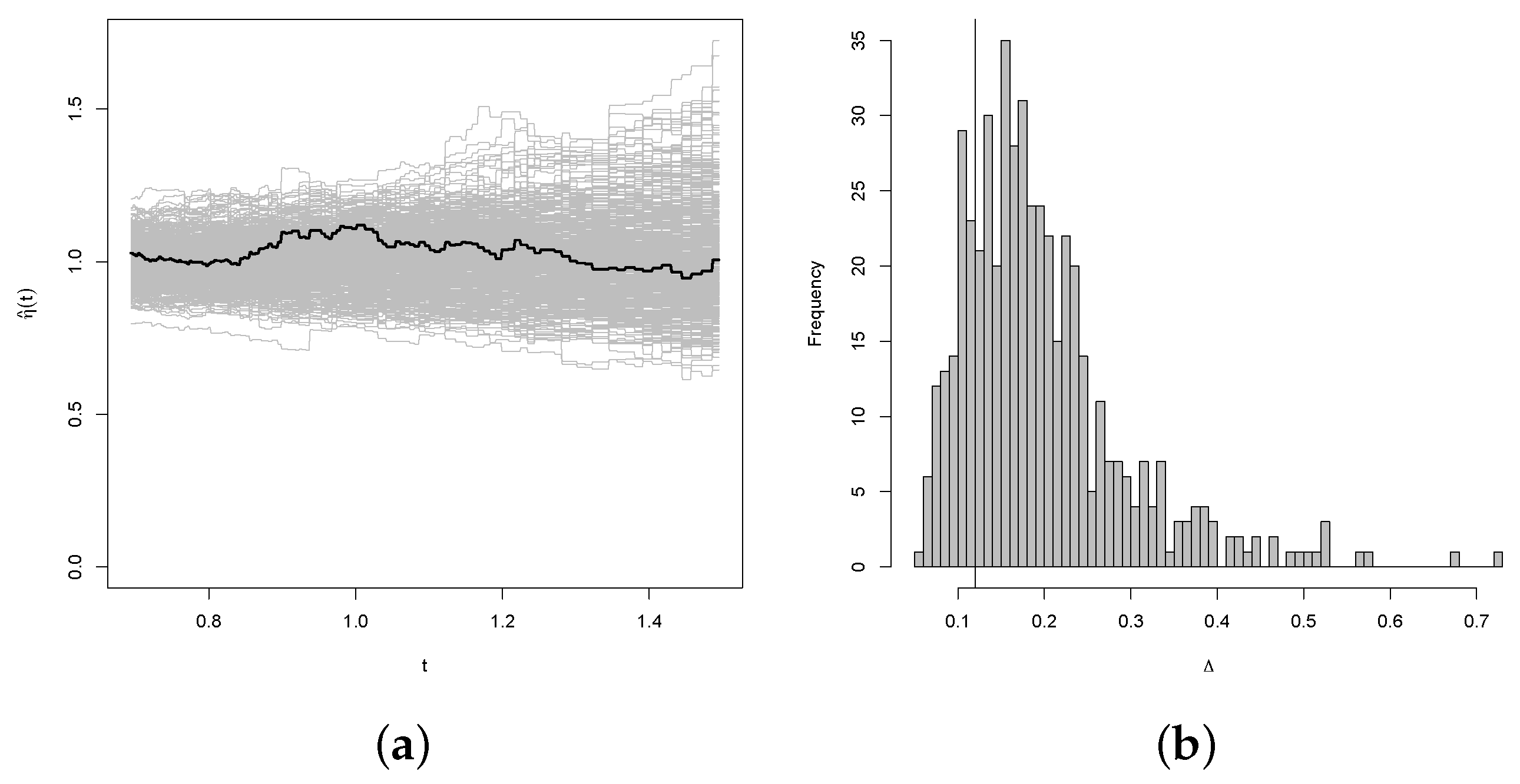
Figure 13.
Results of the bootstrap test of the null hypothesis of exchangeability for the joint distribution of Uranium and Titanium with exponential marginal distributions. The thick line in panel (a) represents the expectation of the simulation. Panel (b) represents the histogram of the simulation.

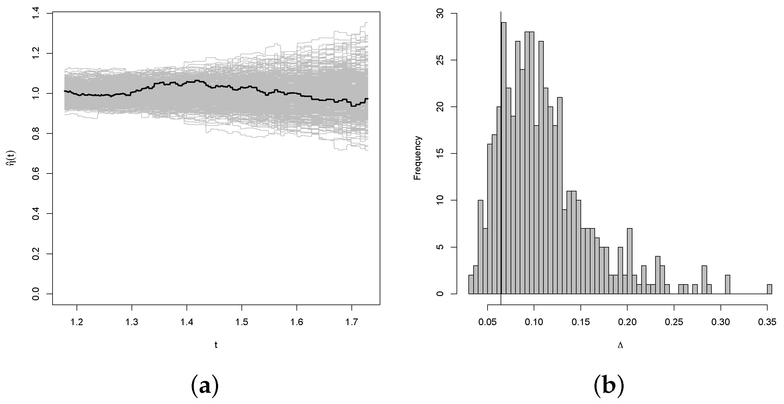
Figure 14.
Results of the bootstrap test of the null hypothesis of exchangeability for the joint distribution of Uranium and Titanium with Weibull marginal distributions. The thick line in panel (a) represents the expectation of the simulation. Panel (b) represents the histogram of the simulation.
Figure 14.
Results of the bootstrap test of the null hypothesis of exchangeability for the joint distribution of Uranium and Titanium with Weibull marginal distributions. The thick line in panel (a) represents the expectation of the simulation. Panel (b) represents the histogram of the simulation.


Table 1.
Bootstrap estimates of the p-values for testing the null hypothesis of Type I tail exchangeability for the chemical concentration data.
Table 1.
Bootstrap estimates of the p-values for testing the null hypothesis of Type I tail exchangeability for the chemical concentration data.
| Chemicals | Marginals | p-Value | |
|---|---|---|---|
| Uranium and Lithium | Pareto | 0.1903 | 0.628 |
| Exponential | 0.1201 | 0.804 | |
| Weibull | 0.0644 | 0.854 | |
| Uranium and Titanium | Pareto | 0.6182 | 0.006 |
| Exponential | 0.6090 | 0.004 | |
| Weibull | 0.4180 | 0.000 |
Disclaimer/Publisher’s Note: The statements, opinions and data contained in all publications are solely those of the individual author(s) and contributor(s) and not of MDPI and/or the editor(s). MDPI and/or the editor(s) disclaim responsibility for any injury to people or property resulting from any ideas, methods, instructions or products referred to in the content. |
© 2024 by the author. Licensee MDPI, Basel, Switzerland. This article is an open access article distributed under the terms and conditions of the Creative Commons Attribution (CC BY) license (https://creativecommons.org/licenses/by/4.0/).
Share and Cite
MDPI and ACS Style
Pramanik, P. Dependence on Tail Copula. J 2024, 7, 127-152. https://doi.org/10.3390/j7020008
AMA Style
Pramanik P. Dependence on Tail Copula. J. 2024; 7(2):127-152. https://doi.org/10.3390/j7020008
Chicago/Turabian StylePramanik, Paramahansa. 2024. "Dependence on Tail Copula" J 7, no. 2: 127-152. https://doi.org/10.3390/j7020008