Approximation of Any Particle Size Distribution Employing a Bidisperse One Based on Moment Matching

Abstract

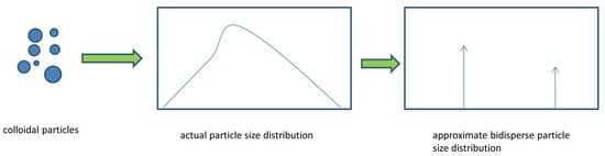
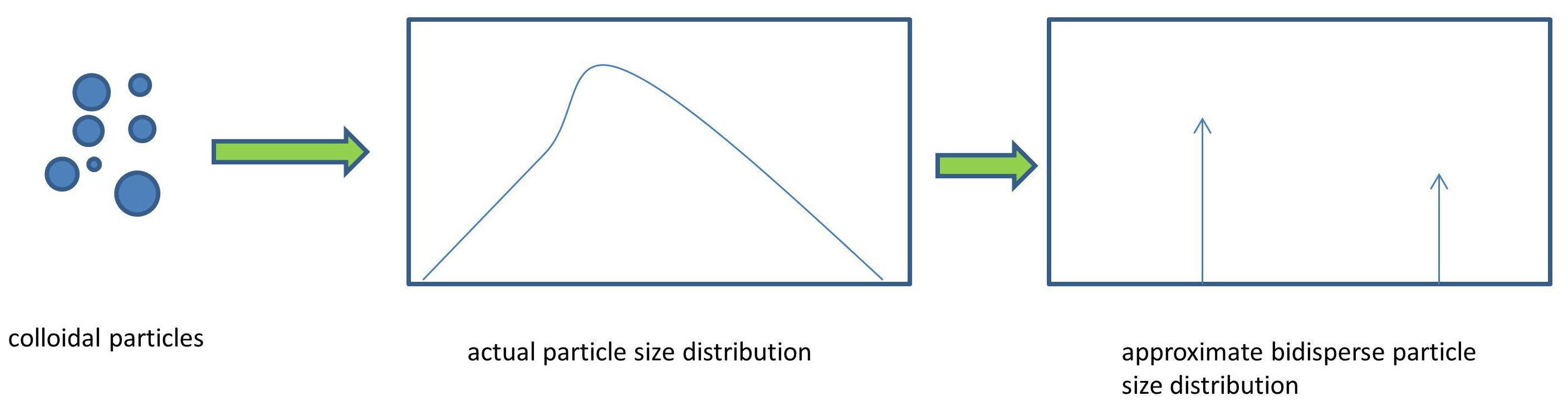
Dispersed phases like colloidal particles and emulsions are characterized by their particle size distribution. Narrow distributions can be represented by the monodisperse distribution. However, this is not the case for broader distributions. The so-called quadrature methods of moments assume any distribution as a bidisperse one in order to solve the corresponding population balance. The generalization of this approach (i.e., approximation of the actual particle size distribution according to a bidisperse one) is proposed in the present work. This approximation helps to compress the amount of numbers for the description of the distribution and facilitates the calculation of the properties of the dispersion (especially convenient in cases of complex calculations). In the present work, the procedure to perform the approximation is evaluated, and the best approach is found. It was shown that the approximation works well for the case of a lognormal distribution (as an example) for a moments order from 0 to 2 and for dispersivity up to 3.

1. Introduction

The basic feature of colloids [1], as for aerosols [2], particulate matter [3], polymers [4], etc., is that they appear in the form of a collection of discrete entities. Each entity may differ from the others in several aspects (shape, composition, etc.). However, in order to describe it, a certain number of variables is needed. These variables are called descriptors or internal coordinates of the entity. Several such descriptors have been used in the relevant literature (aspect ratio, fractal dimension, and surface area). However, in the simplest case of a single descriptor, one representative of the size of the entity is employed. Typically, this descriptor can be the length, equivalent diameter, volume, mass, or molecular weight (in the case of polymers).

Let us consider the case of a single descriptor in which the volume of the entity is selected (equivalent to particle mass for particles of constant density). The usual approach of a single descriptor refers to the choice of the entity’s (equivalent) diameter or the entity’s volume. Typically, the diameter is chosen in cases of gas–liquid dispersions [5], emulsions [6], and crystallization [7], and the volume is chosen in cases of aerosols [8] and precipitation [9]. The above comment does not refer to measurement techniques but rather how the subject of distributions and the governing equations are developed in the relevant scientific discipline. The volume is an intrinsic particle variable, and no approximation is needed to describe it (e.g., like the equivalent diameter); it is exactly conserved during a coagulation event. This renders it appropriate for use in theoretical tools, such as population balance equations. From now on, the term “entity” will be replaced by the term “particle”, as it refers to a colloidal system (dispersion or emulsion). In general, the particle population is described by a density function, which expresses how the population is distributed with respect to the internal variable (i.e., particle volume in the present case). The distributed variable can be the particle number, surface, or volume, with the number being the one most extensively used in the literature. In particular, the function f(x) is the number concentration of particles with sizes between x and x + dx. The function f(x) is a number density function, so its units are numbers per length in the sixth power, i.e., #/m⁶. According to the above discussion, the particle number and particle volume are chosen as dependent and independent variables of the particle size distribution, respectively. However, the extension of the methodology to other pairs of variables is possible.

It is common knowledge that every property of the dispersion can be computed by invoking the particle size distribution (i.e., the function f(x)). The problem with the function f(x) is that it must be known at several values of x in order to have its fine discrete representation. This creates problems for calculations regarding properties of the dispersion. The most extensively discussed example in the literature is a case where f(x) is a local flow field variable, which implies that it depends on the spatial coordinate and on time. In general, knowledge of the discrete form of f(x) can be replaced by knowledge of its main features. The particle size distribution can be characterized hierarchically by three main variables: the total particle number concentration, the average particle volume, and particle polydispersity. In the case of low polydispersity, the monodisperse approximation has been proved successful in several fields of application [10]. However, in the case of high polydispersity, a measure of this polydispersity is necessary. This is achieved either by assuming a specific shape of the distribution (i.e., lognormal, Gamma, Weibull, etc. [11,12,13]) or by assuming a bidisperse distribution approximating the actual one according to the sum of two discrete particle sizes. It is noted that the above distributions have been used in the context of population balance equation solutions. Here, the aim is to compress the information contained in the actual particle size distribution. The bidisperse distribution according to the terminology of the present work is one that consists of two discrete particle sizes, and this differs from a bimodal distribution consisting of several sizes (it could be said to have two peaks, but it is subjective because the existence of peaks depends on the way of presenting the distribution (e.g., volume- or number-based).

This work intends to show how successful the bidisperse distribution is to approximate arbitrary particle size distributions. The main focus is not the best approximation of the actual distribution but the optimization of its simplest approximation. As a benchmark case, a lognormal size distribution is considered, as it is the most usual shape for the characterization of particulate distributions. The meaning of approximation must be discussed. In what sense is the actual measured distribution approximated by a bidisperse one? The answer is that the approximation must be performed with respect to the moments of the distribution. Many properties of the particulate system are expressed in terms of the moments of the distribution, e.g., the length, area, volume, scattering, etc. Knowledge of these quantities is usually more important than detailed size distribution knowledge. In addition, there are other properties that depend on integrals over the size distribution with more complex kernels. Even in this case, a good approximation of the moments of the distribution (in particular, in a finite range of orders) ensures the reliable calculation of the properties based on the approximate distribution. The structure of the present work is as follows. First, the mathematical problem is formulated, and then the numerical results are presented, followed by an extensive discussion and specific suggestions for real distribution approximation according to bidisperse one.

2. Methods

In order to simplify the analysis and to facilitate the numerical calculations, the normalized particle size distribution F(η) (where η = x/x_av and x_av is the average volume of the particles) will be employed. The way to transform the actual distribution f(x) to the normalized F(η) is the following. At first, the following moments of the actual distribution are computed:

$$\mathrm{N}={\displaystyle \underset{0}{\overset{\infty }{\int }}\mathrm{f}(\mathrm{x})\mathrm{d}\mathrm{x}}, \mathrm{M}={\displaystyle \underset{0}{\overset{\infty }{\int }}\mathrm{x}\mathrm{f}(\mathrm{x})\mathrm{d}\mathrm{x}}$$

(1)

Then, x_av = M/N is computed, and the normalized distribution is found from the relation F(η) = x_avf(ηx_av)/N. The normalized moments of order i (i can be any rational number and not necessarily an integer) of the particle size distribution are defined as

$${\mathrm{M}}_{\mathrm{i}}={\displaystyle \underset{0}{\overset{\infty }{\int }}{\mathsf{\eta }}^{\mathrm{i}}\mathrm{F}(\mathsf{\eta })\mathrm{d}\mathsf{\eta }}$$

(2)

By constructing the two moments, M_o and M₁ are equal to unity. The whole particle population is characterized now by two numbers N, x_av and the function F(η), instead of the function f(x) alone. As a prototype to assess the validity of the bidisperse distribution, the lognormal distribution will be considered here. The reason for this particular choice is that this distribution is the most extensively used in the literature of dispersions, and its parameters are directly related to specific features of the distribution (e.g., average particle volume, polydispersity). This is not the case for other candidate distributions, such as the Gamma one.

The normalized shape of the lognormal distribution is the following [8]:

$$\mathrm{F}(\mathsf{\eta })=\frac{1}{\sqrt{2\mathsf{\pi }\mathrm{s}}}\frac{1}{\mathsf{\eta }}\exp (-\frac{1}{2\mathrm{s}}{(\ln (\mathsf{\eta })+\frac{\mathrm{s}}{2})}^2)$$

(3)

The parameter s is called “dispersivity”, and it is the measure of the polydispersity of the distribution. Using the above expression, the moments of the distribution can be computed in closed form as:

$${\mathrm{M}}_{\mathrm{i}}=\exp (\frac{{\mathrm{i}}^2-\mathrm{i}}{2}\mathrm{s})$$

(4)

The simplest approximation of the distribution is the monodisperse one in which F(η) = δ(η − 1), where δ is the so-called Dirac delta function. This approximation suggests that all of the particles have a size equal to the average size of the distribution. This approximation has been proved to be useful in several cases; however, the lack of any information regarding the broadness of the distribution is evident. The next level of approximation is the bidisperse distribution. It is important to clarify here the meaning of the terms “unimodal/bimodal” and “monodisperse/bidisperse” distributions. The first term refers to the number of peaks of the distribution (which holds for smooth distributions only), whereas the second refers to the number of different sizes of particles.

The concept of the bidisperse distribution has been extensively used (although it is not recognized as such) by the so-called quadrature methods of moments used for the solution of population balance equations [14,15]. The equation is integrated numerically using the bidisperse distribution to advance four moments of the distribution. At each time step, the four features of the bidisperse distribution are found by matching the four moments. A specific algorithm exists for this second step (i.e., the product difference algorithm), but here it is preferred to keep the original algebraic structure of the problem for generality.

The bidisperse distribution has the form F(η) = w₁δ(η − η₁) + w₂δ(η − η₂), where the four unknowns (w₁, w₂, η₁, and η₂) have to be found considering the known moments of the distribution. Let us assume that moments in the range 0 ≤ i ≤ 2 are of interest. This choice refers to reliable calculations not only of the moments themselves but also for integral properties containing more complex kernels not locally exceeding the range of i. The next step is to choose the four moments for the matching procedure. In principle, any quartet of moments with no orders that are very close to each other can be used. The moments of order i = 0 and i = 1 are chosen here due to their physical meaning (the total particle number and mass), and the moment i = 2 because it is at the end of the i-domain of interest. One moment is missing, and there is not an obvious choice. Let us call k the order of the fourth moment. The system of equations to be solved for the bidisperse parameters is

$${\mathrm{w}}_1+{\mathrm{w}}_2=1$$

(5)

$${\mathrm{w}}_1{\mathsf{\eta }}_1+{\mathrm{w}}_2{\mathsf{\eta }}_2=1$$

(6)

$${\mathrm{w}}_1{\mathsf{\eta }}_1^2+{\mathrm{w}}_2{\mathsf{\eta }}_2^2={\mathrm{e}}^{\mathrm{s}}$$

(7)

$${\mathrm{w}}_1{\mathsf{\eta }}_1^{\mathrm{k}}+{\mathrm{w}}_2{\mathsf{\eta }}_2^{\mathrm{k}}={\mathrm{e}}^{\frac{{\mathrm{k}}^2-\mathrm{k}}{2}\mathrm{s}}$$

(8)

In case of arbitrary particle size distribution, the above system holds, but the right-hand sides of Equations (7) and (8) are M₂ and M_k, respectively, where M_i is the i-th moment of the distribution, numerically computed.

Fortunately, one can proceed analytically with the above system. The first two equations comprise a linear system for w₁, w₂, which can be solved to give

$${\mathrm{w}}_1=\frac{{\mathsf{\eta }}_2-1}{{\mathsf{\eta }}_2-{\mathsf{\eta }}_1}$$

(9)

$${\mathrm{w}}_2=\frac{1-{\mathsf{\eta }}_1}{{\mathsf{\eta }}_2-{\mathsf{\eta }}_1}$$

(10)

Substitution of the above Equations (9) and (10) in Equation (7), after some algebra, a trinomial equation for η₂ results. Upon solving this equation and retaining only the one root with an addition sign (because only the root with η₂ > 1 is of interest), the following relations result:

$${\mathsf{\eta }}_2=\frac{-\mathrm{A}+{({\mathrm{A}}^2-4\mathsf{\Gamma })}^{1/2}}{2}$$

(11)

where

$$\mathrm{A}=\frac{{\mathsf{\eta }}_1^2-{\mathrm{e}}^{\mathrm{s}}}{1-{\mathsf{\eta }}_1}$$

(12)

$$\mathsf{\Gamma }=\frac{{\mathrm{e}}^{\mathrm{s}}{\mathsf{\eta }}_1-{\mathsf{\eta }}_1^2}{1-{\mathsf{\eta }}_1}$$

(13)

After substituting Equations (11)–(13) to Equation (8), a single transcendental equations for η₁ arises. This single equation has to be solved numerically. The different scenarios of moment matching presented in the results will be named to facilitate the discussion. The four moments matching with k = 0.5 are named Case 1. A similar scenario with k = 1.5 (instead of k = 0.5) is called Case 2.

Other ways of performing moment approximation with simple matching are also examined here. In order to present them, let us define the measure P denoting the total quality of approximation of moments in the range of i between 0 and 2.

$$\mathrm{P}=\frac{1}{2}{\displaystyle \underset{0}{\overset{2}{\int }}\left|1-\frac{{\mathrm{M}}_{\mathrm{b}\mathrm{i}}}{{\mathrm{M}}_{\mathrm{i}}}\right|}\mathrm{d}\mathrm{i}$$

(14)

where M_bi is the normalized moment of the bidisperse distribution computed as

$${\mathrm{M}}_{\mathrm{b}\mathrm{i}}={\mathrm{w}}_1{\mathsf{\eta }}_1^{\mathrm{i}}+{\mathrm{w}}_2{\mathsf{\eta }}_2^{\mathrm{i}}$$

(15)

The reason for which the integrand is not just the difference between exact and approximate moments is that the moments increase abruptly in the region of i = 2, so there would be a bias to reduce the deviation mostly at this region. The normalized deviation used ensures uniform approximation through the domain of i from 0 to 2. The measure P can be decomposed to measures P₁ and P₂ (2P = P₁ + P₂), defined as follows:

$${\mathrm{P}}_1={\displaystyle \underset{0}{\overset{1}{\int }}\left|1-\frac{{\mathrm{M}}_{\mathrm{b}\mathrm{i}}}{{\mathrm{M}}_{\mathrm{i}}}\right|}\mathrm{d}\mathrm{i}$$

(16)

$${\mathrm{P}}_2={\displaystyle \underset{1}{\overset{2}{\int }}\left|1-\frac{{\mathrm{M}}_{\mathrm{b}\mathrm{i}}}{{\mathrm{M}}_{\mathrm{i}}}\right|}\mathrm{d}\mathrm{i}$$

(17)

The scenario of Case III includes matching for i = 0, 1 (i.e., use of Equations (9) and (10)) and minimization of P with respect to variables η₁, η₂. Finally, the scenario of Case 4 refers to matching for i = 0, 1, 2 (i.e., use of Equations (11)–(13)) and minimizing the expression $\mathrm{P}+\left|{\mathrm{P}}_1-{\mathrm{P}}_2\right|$ with respect to η₁.

3. Results

A lognormal distribution with dispersivity s is assumed, and it is approximated according to a bidisperse one using one of the procedures for Cases 1–4. Then, the moments of order i for 0 ≤ i ≤ 2 are calculated for the bidisperse distribution and compared to those of the lognormal distribution. The range of dispersivity used in the calculations is from 0.3 to 3, with s = 0.3 corresponding to a very narrow distribution and s = 3 corresponding to a very broad distribution.

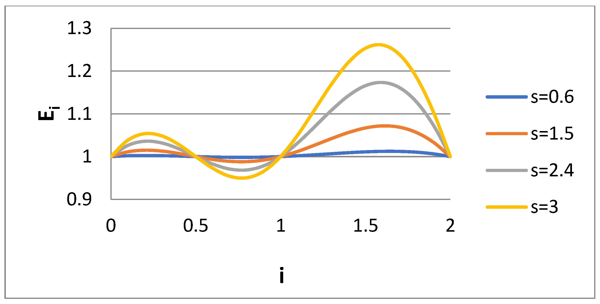
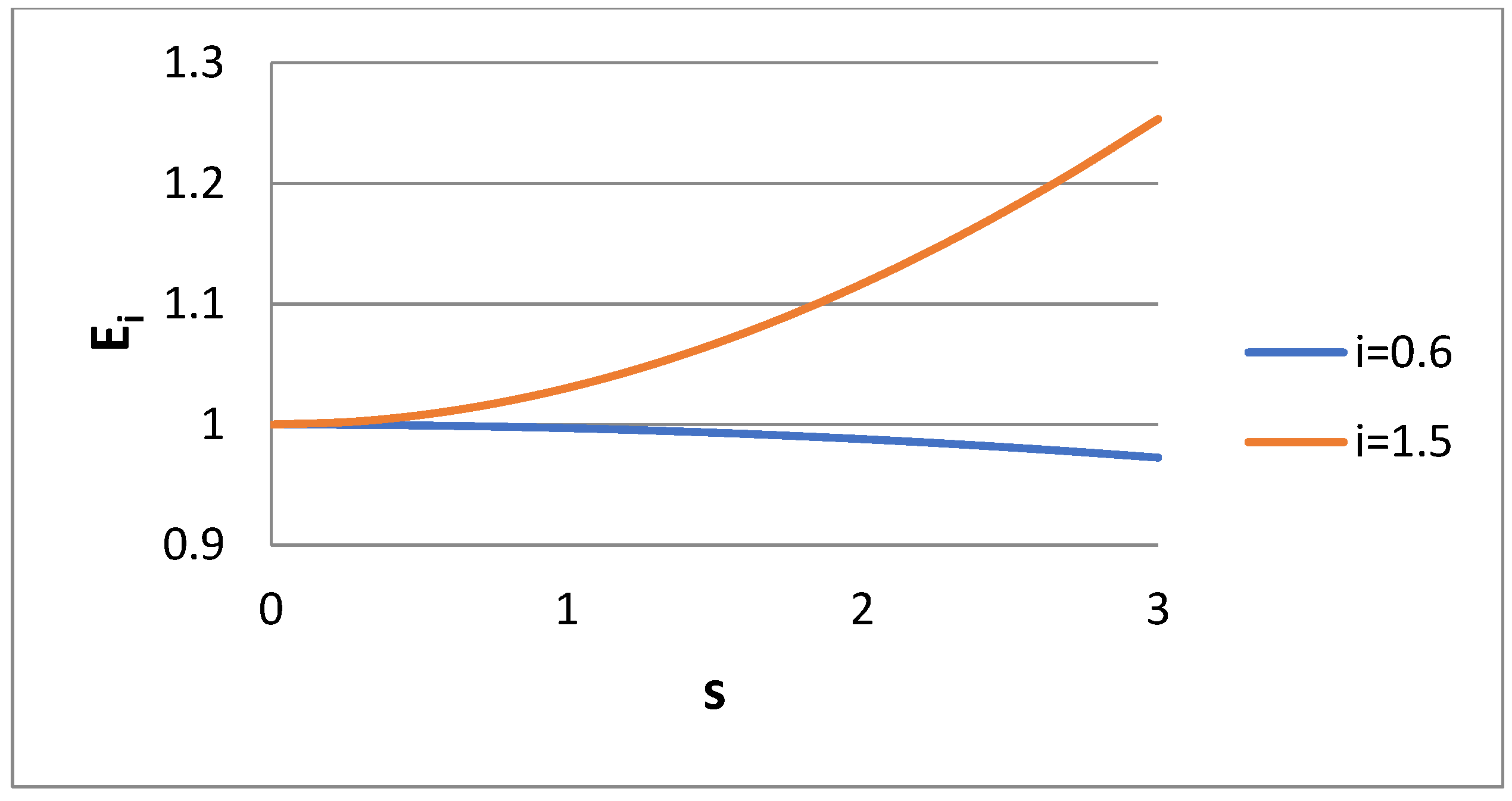
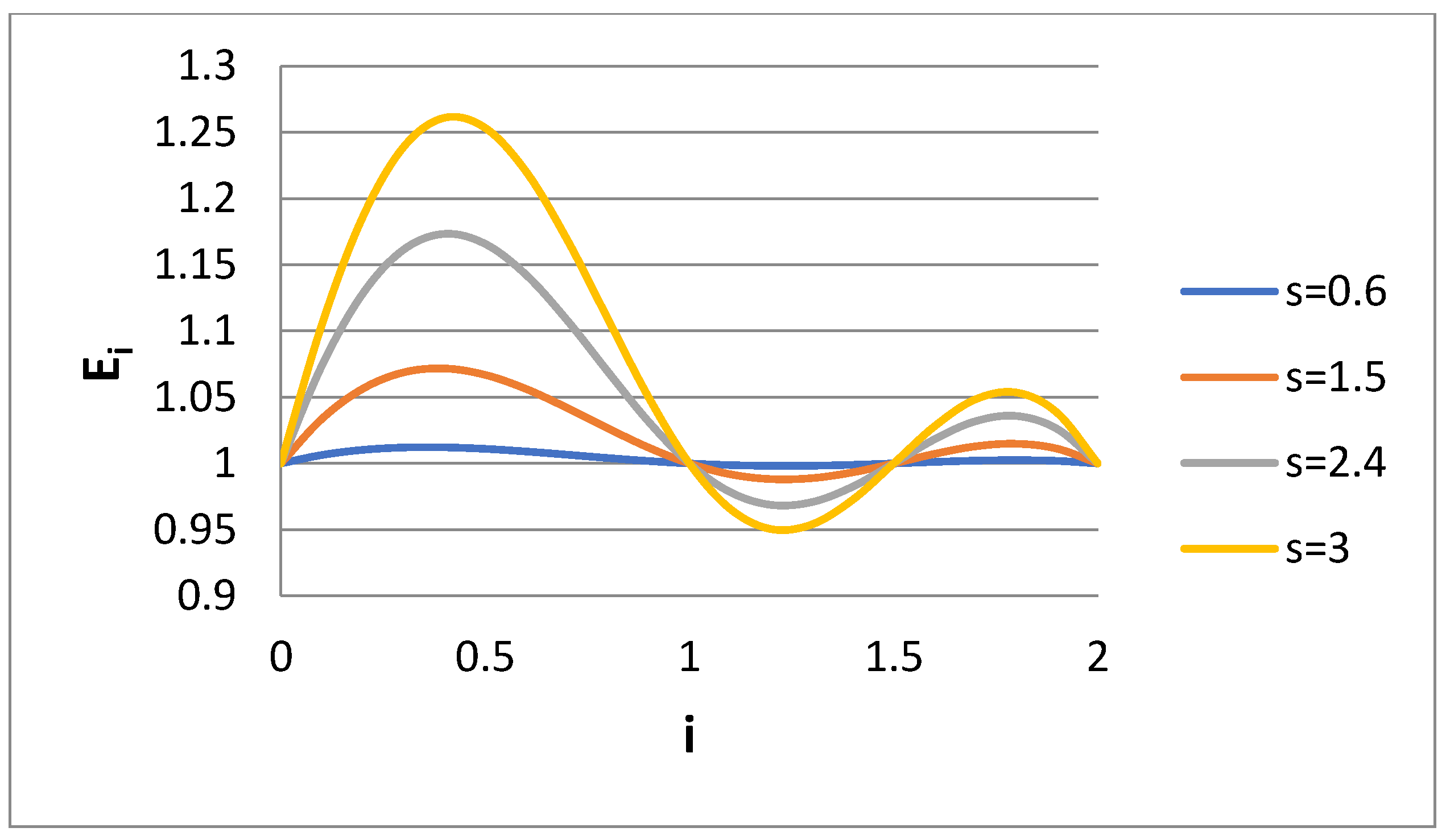
A basic variable presented in the results is the ratio of approximate (bidisperse) to exact (log normal) moment of order I, i.e., E_i = M_bi/M_i. This ratio is shown versus i in Figure 1 for the Case 1 scenario and for several values of dispersivity s of the lognormal distribution. The error of approximating the lognormal distribution according to a bidisperse one is zero for the moments i = 0, 1, 2, 0.5, as expected. Also, the error increases as the spread of the lognormal distribution (i.e., s) increases. The interesting thing is that whereas the error in the range 0 < I < 1 is kept low (due to the choice k = 0.5), the error in region 1 < i < 2 is much higher, with a peak at i = 1.5. The variable E_i is shown as the function of dispersivity for i = 0.6 and i = 1.5 in Figure 2. In line with Figure 1, it seems that E_i decreases with s for i = 0.6 and increases with s for i = 1.5.

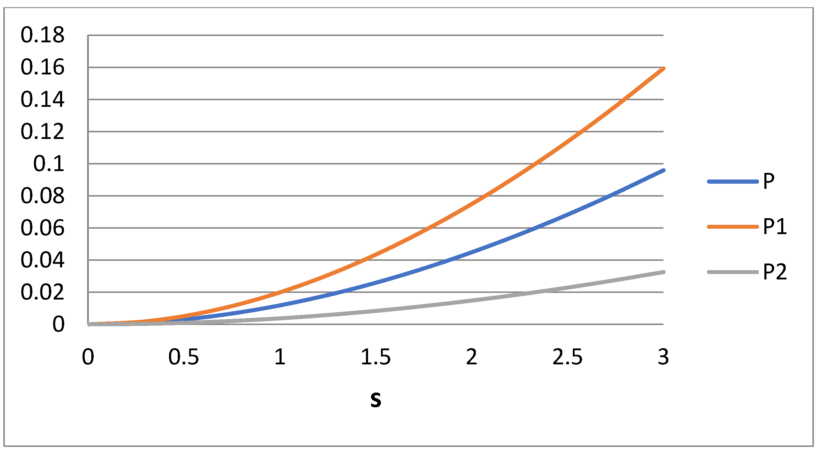
Given the above behavior of E_i for the Case 1 scenario, it would be of interest to check what happens in the Case 2 scenario (k = 1.5). The variable E_i is presented versus i for several s values for Case 2 in Figure 3. The value E_i = 1 in i = 0.5 has been replaced by the value E_i = 1 at i = 1.5. It appears that Figure 1 and Figure 3 show some kind of symmetry (e.g., rotation around axis i = 1). It is obvious that the choice of the fourth matching moment is quite crucial for the accuracy of the calculated moments through bidisperse approximation. If one is interested in the computation of the specific moment i = m, then the matching must be performed for the moments i = 0, 1, 2, m. The question is what is the right choice in a case where no specific moment is of interest but rather a whole range of moments. Let us observe how the integral error measures P, P₁, and P₂ behave in Case 2. The dependence of variables P, P₁, and P₂ on s for Case 2 is shown in Figure 4. It can be said that P denotes the total error of the approximation in the moment region 0 ≤ i ≤ 2, whereas P₁ and P₂ denote the errors at i intervals 0 ≤ i ≤ 1 and 1 ≤ i ≤ 2, respectively. The average error in the moments approximation does not exceed 10% (i.e., 0.1). The problem is that this error is quite unevenly distributed in the domain of interest. The curves for P₁ and P₂ reveal that the error in domain 1 (0 ≤ i ≤ 1) is about five times larger than the error in domain 2 (1 ≤ i ≤ 2). The opposite trend appears in Case 1.

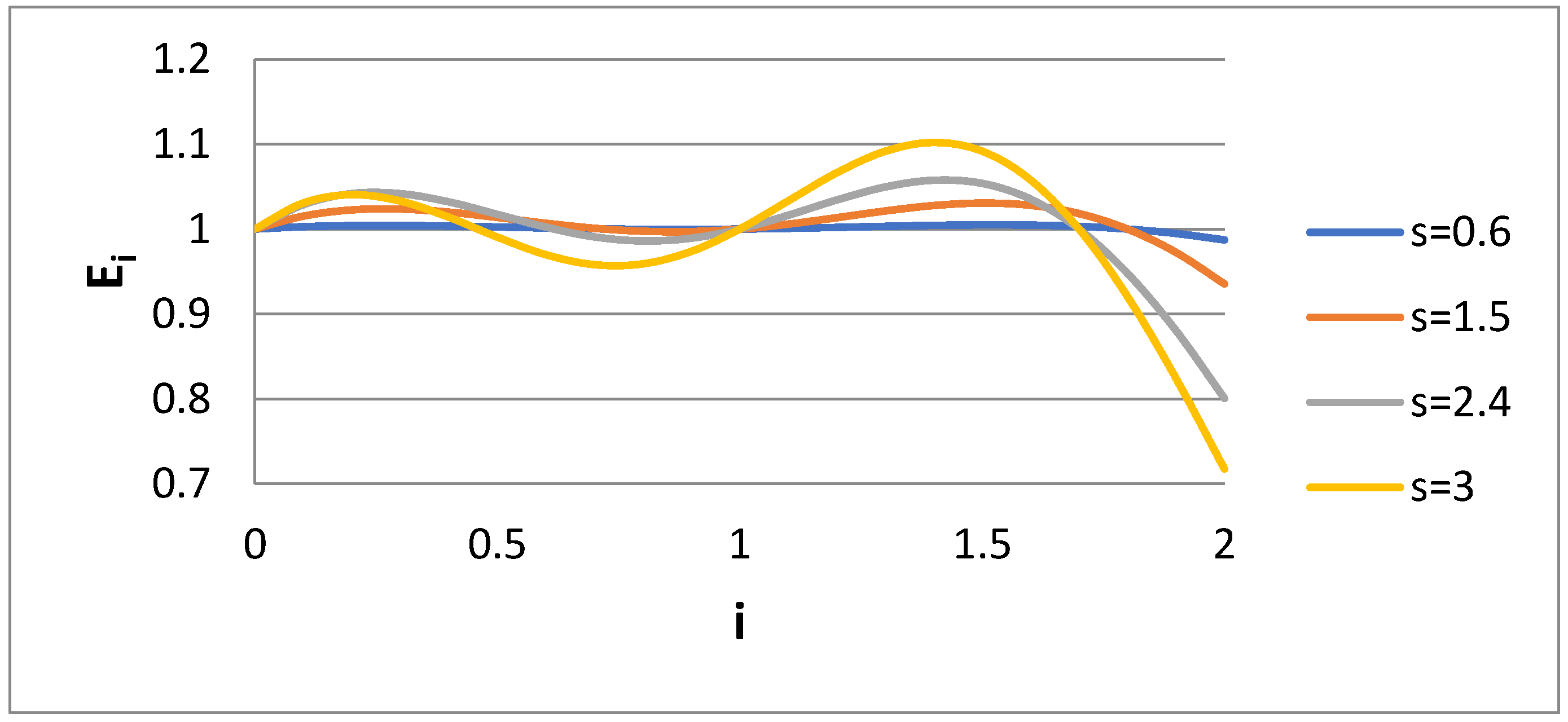
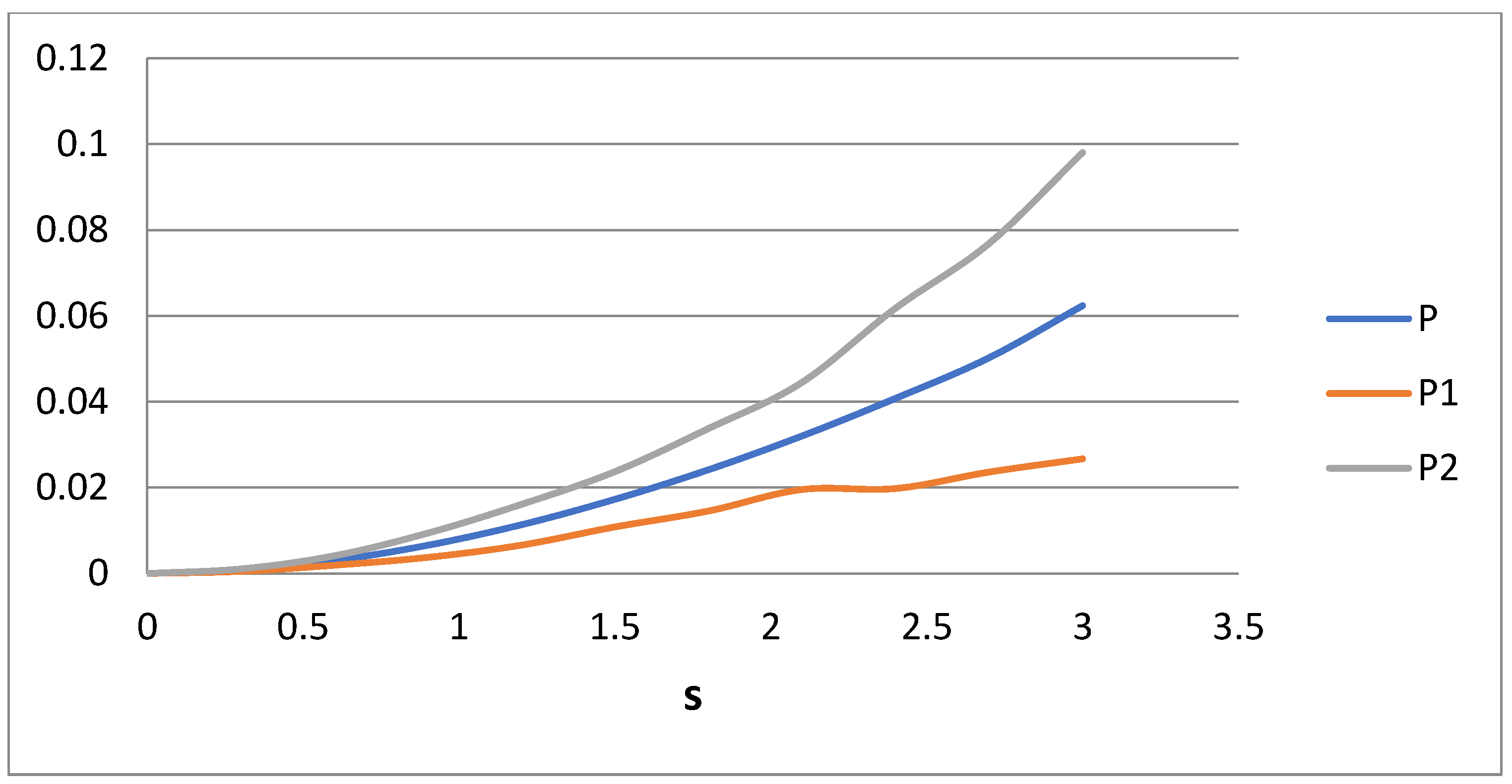
The next step is to explicitly require the minimization of P instead of matching the moments. In order to increase the versatility of the minimization scheme, matching is performed only for i = 0 and 1, and the minimization of P is achieved with respect to the two parameters η₁ and η₂. The values of E_i versus i for Case 3 are shown in Figure 5. In Figure 6, the measures for P, P₁, and P₂ are shown versus s. It appears that Case 3 leads to smaller overall error, but the non-uniformity of the error is still uneven. The most important thing is that according to Figure 6, the largest deviation appears at the value i = 2. There are some slope discontinuities at the P curves, possibly due to the trapping of the minimization process at local shallow minimums close to the global one.

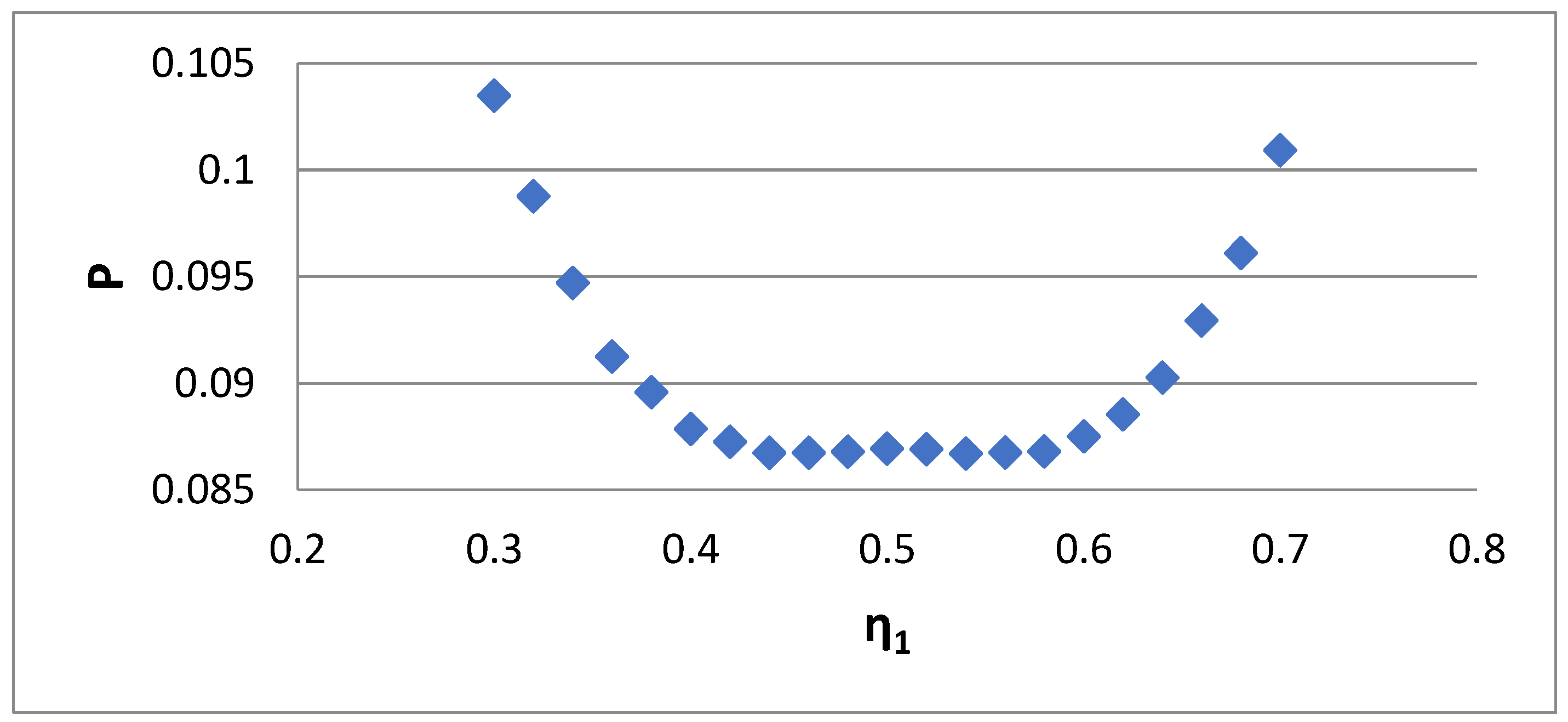
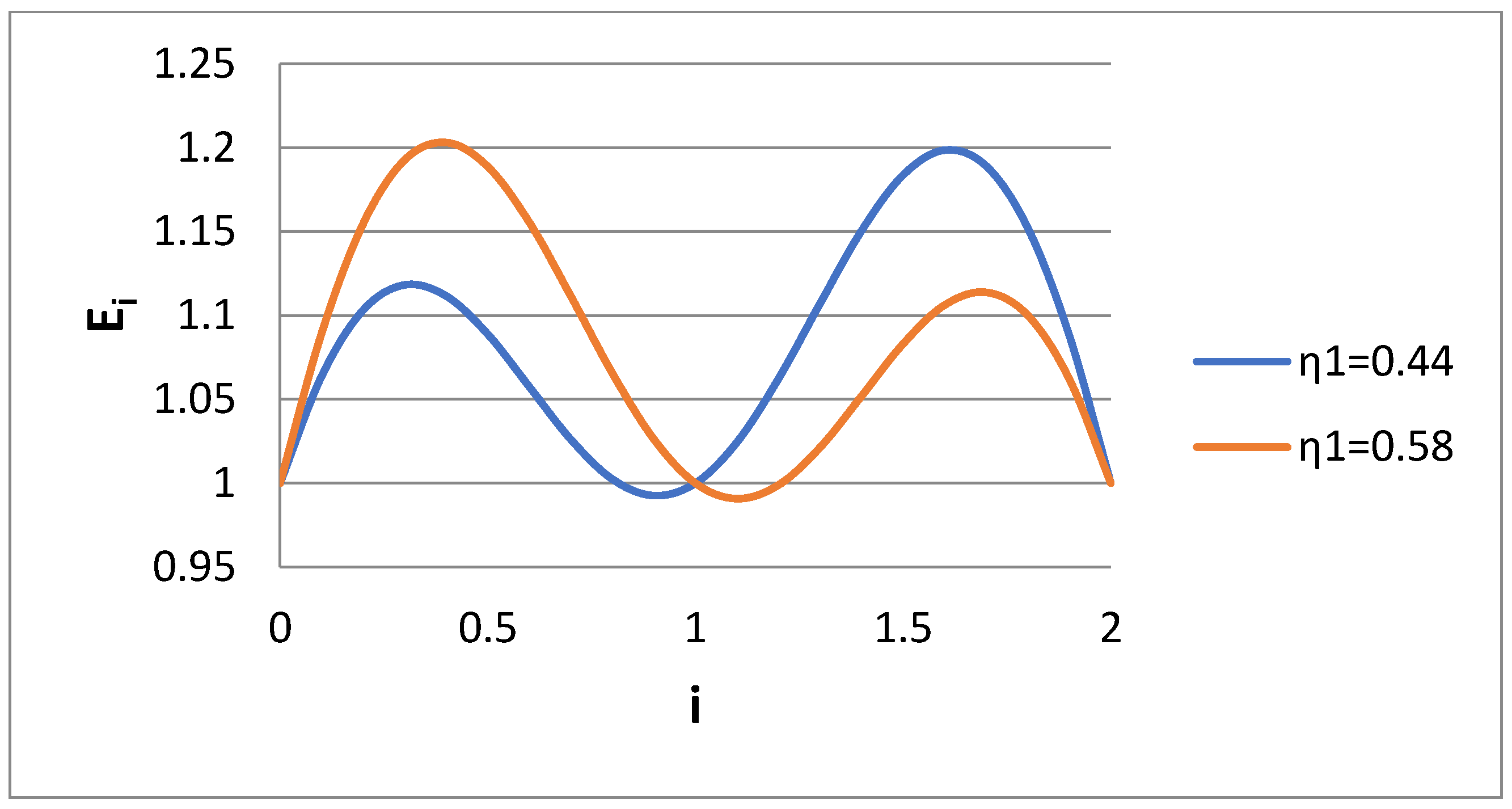
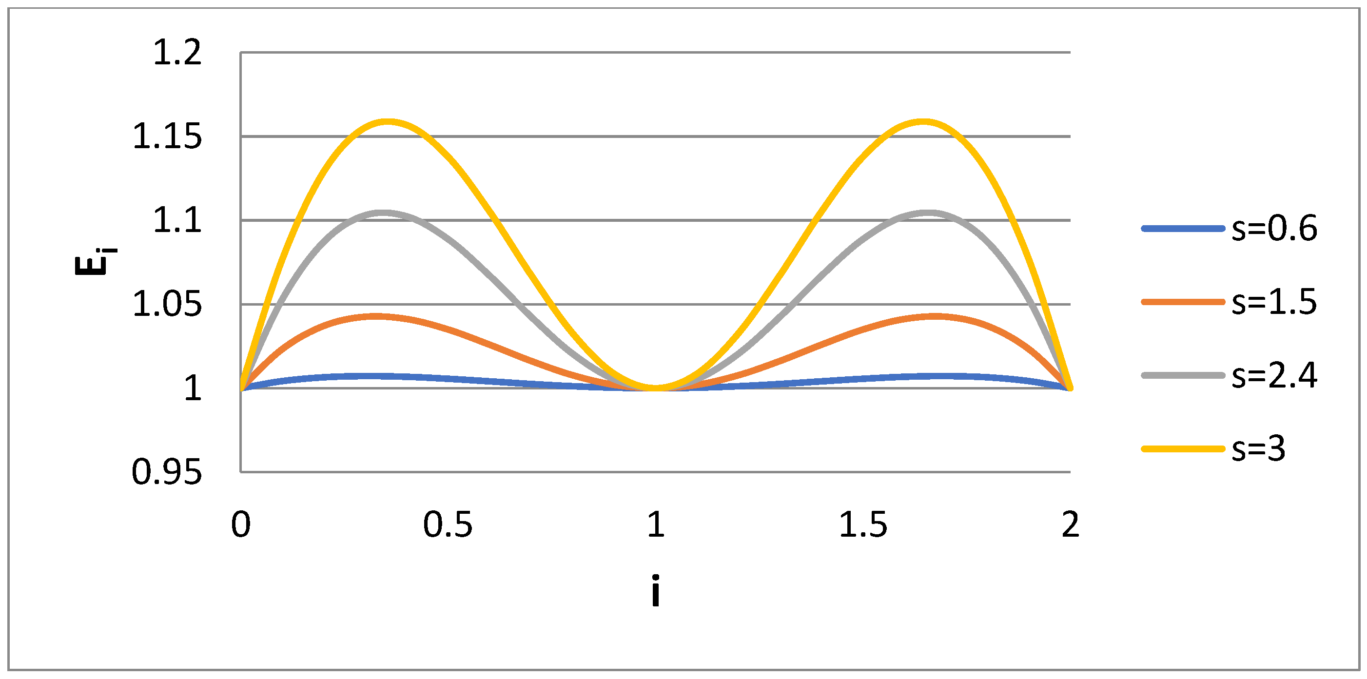
So, Case 3 is the best choice for extracting bidisperse distribution properties, except if one has a special interest in the i = 2 moment. In this situation, the scenario of Case 4 is followed. The matching is performed for i = 0, 1, 2, and the variable η₁ is found from the minimization of some objective function. This function cannot be P because, as shown in Figure 7, there is a whole region of η₁ in which P is almost constant. The absolute minimum values correspond to uneven errors. For example, the error distribution for two values of η₁ appears in Figure 8. The uneven error distribution is obvious. The symmetric error actually occurs at a local maximum of the P function (see Figure 7). The symmetric error distribution appears in Figure 9. The particular value of η₁ is found by minimizing the function:

$$\mathsf{\Phi }=\mathrm{P}+\left|{\mathrm{P}}_1-{\mathrm{P}}_2\right|$$

(18)

The same result can also be obtained through minimization of the function:

$$\mathsf{\Psi }={\displaystyle \underset{0}{\overset{2}{\int }}{\left(1-\frac{{\mathrm{M}}_{\mathrm{b}\mathrm{i}}}{{\mathrm{M}}_{\mathrm{i}}}\right)}^2}\mathrm{d}\mathrm{i}$$

(19)

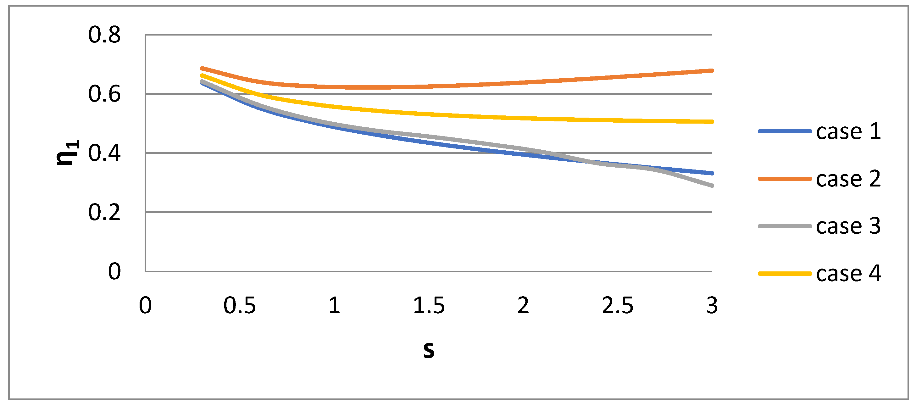
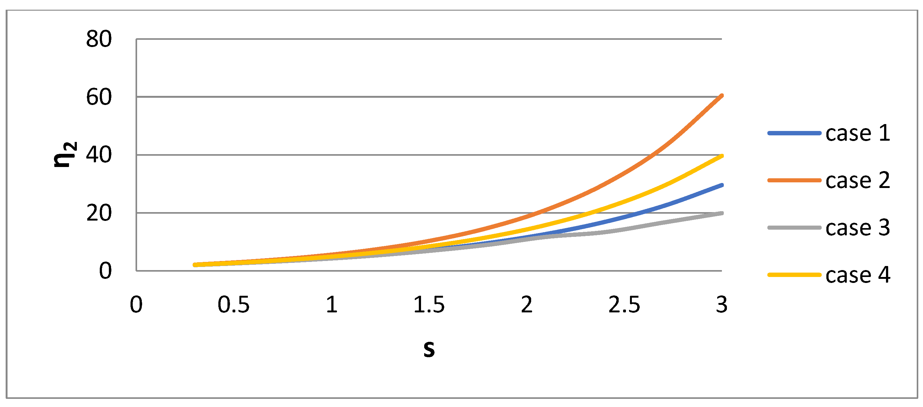
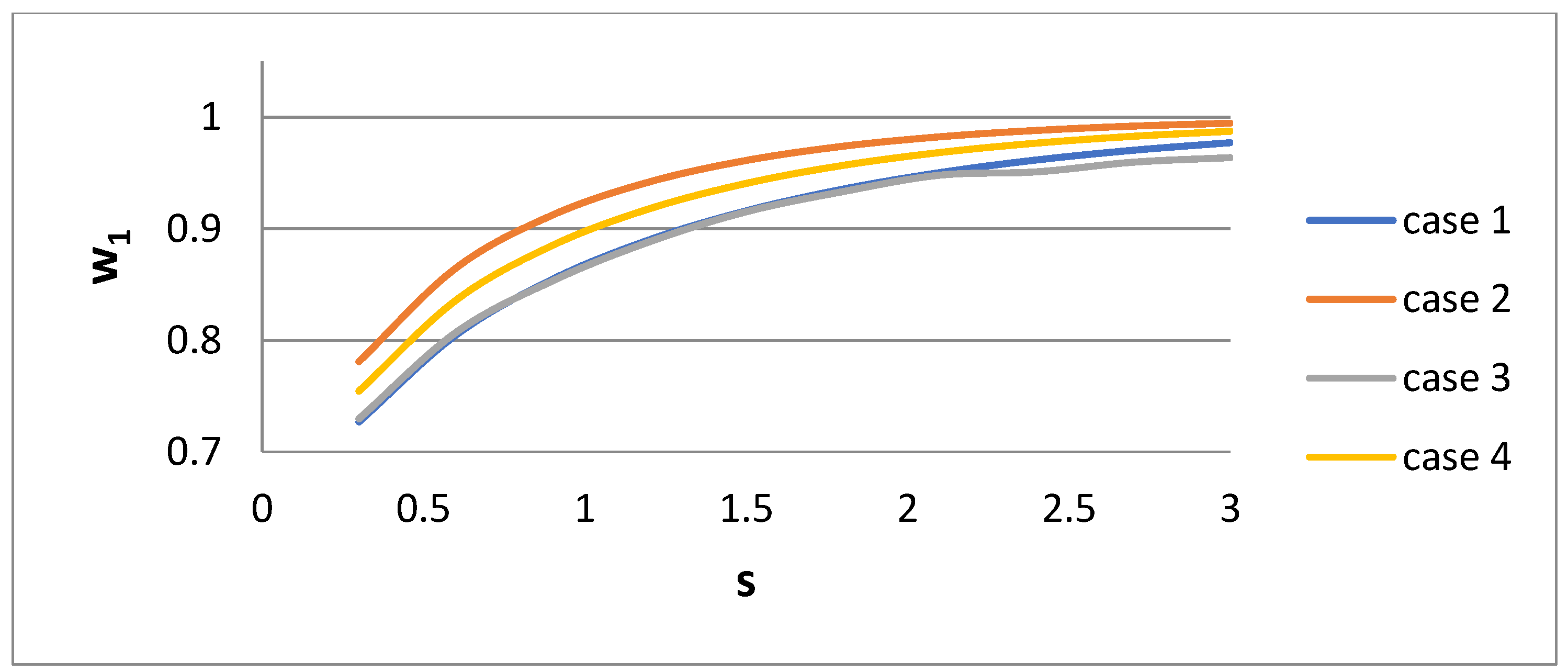
The parameters w₁, η₁, and η₂ of the bidisperse distribution versus dispersivity s for the four cases of their derivation are presented in Figure 10, Figure 11 and Figure 12, respectively. It is interesting that the parameter values are very sensitive to the procedure of their derivation. The parameter η₂ increases rapidly with s. The parameter η₁ exhibits a more complex behavior. It decreases with s for Cases 1, 3, and 4, and there is a non-monotonic behavior for Case 2. It is expected that as the polydispersity increases, the distance between the two sizes of the bidisperse distribution increases. The parameter w₁ increases towards unity as s increases.

The Newton–Raphson technique was used for the algebraic equation solution, and the conjugate gradient method was used for the minimization [16]. There are severe convergence problem in both cases. The convergence was ensured in the present work through an analytical continuation approach. The problem is solved for s = 0.3, and then s starts to increase stepwise when using as initial values for the calculation the convergent values of the parameters from the previous step of s.

The suggested choice for derivation of the bidisperse distribution is Case 4. The average error of the moments 0 < i < 2 is 10% (i.e., 0.1), but the local error can reach 15% (i.e., 0.15) at the maximum distance from the matching moments. In general, the local error decreases for moment order close to the matching values i = 0, 1, 2. In order to get rid of any numerical analysis calculation, the following fitting is performed for the value of η₁ (0 < s < 3):

$${\mathsf{\eta }}_1=0.00977{\mathrm{s}}^4-0.0822{\mathrm{s}}^3+0.262{\mathrm{s}}^2-0.3904\mathrm{s}+0.7574$$

(20)

4. Further Discussion

In this section, the extension of the approach to arbitrary particle size distribution is presented. In addition, the benefit of using the bidisperse approximation in Monte Carlo simulations for computing quantities associated with the distribution, is pointed out. Although the above development and derivation have been made for a lognormal distribution as the prototype, the results of the present work can be generalized to arbitrary particle size distributions. The above procedure of deriving a bidisperse approximation appears complicated because it includes several normalization and mathematical steps. In order to render the results useful for anyone, an example of application of the procedure is given here. Let us say that the dimensional volumes x_j of N particles (j = 1, 2,… N) have been measured. The average volume x_av and the dispersivity s can be found as:

$${\mathrm{x}}_{\mathrm{a}\mathrm{v}}=\frac{{\displaystyle \sum _{\mathrm{j}=1}^{\mathrm{N}}{\mathrm{x}}_{\mathrm{j}}}}{\mathrm{N}}$$

(21)

$$\mathrm{s}=\ln (\frac{\mathrm{N}{\displaystyle \sum _{\mathrm{j}=1}^{\mathrm{N}}{\mathrm{x}}_{\mathrm{j}}^2}}{{({\displaystyle \sum _{\mathrm{j}=1}^{\mathrm{N}}{\mathrm{x}}_{\mathrm{j}}})}^2})$$

(22)

In a case where s < 3, no numerical analysis is needed. The parameter η₁ is found from Equation (20), the parameter η₂ is found from Equations (11)–(13), and the parameter w₁ is found from Equation (9). For s > 3, the minimization problem of Function (18) must be solved combined with Equations (9)–(13). Finally, the two characteristic volumes of the bidisperse distribution are η₁x_av and η₂x_av. The number fraction of the type “1” particles is w₁. It is noted that the above approach is based on the assumption that the actual distribution has a shape close to the lognormal one. Otherwise, the procedure must be performed by assuming the numerically computed moments of the actual distribution in Equation (14) instead of those of the lognormal distribution.

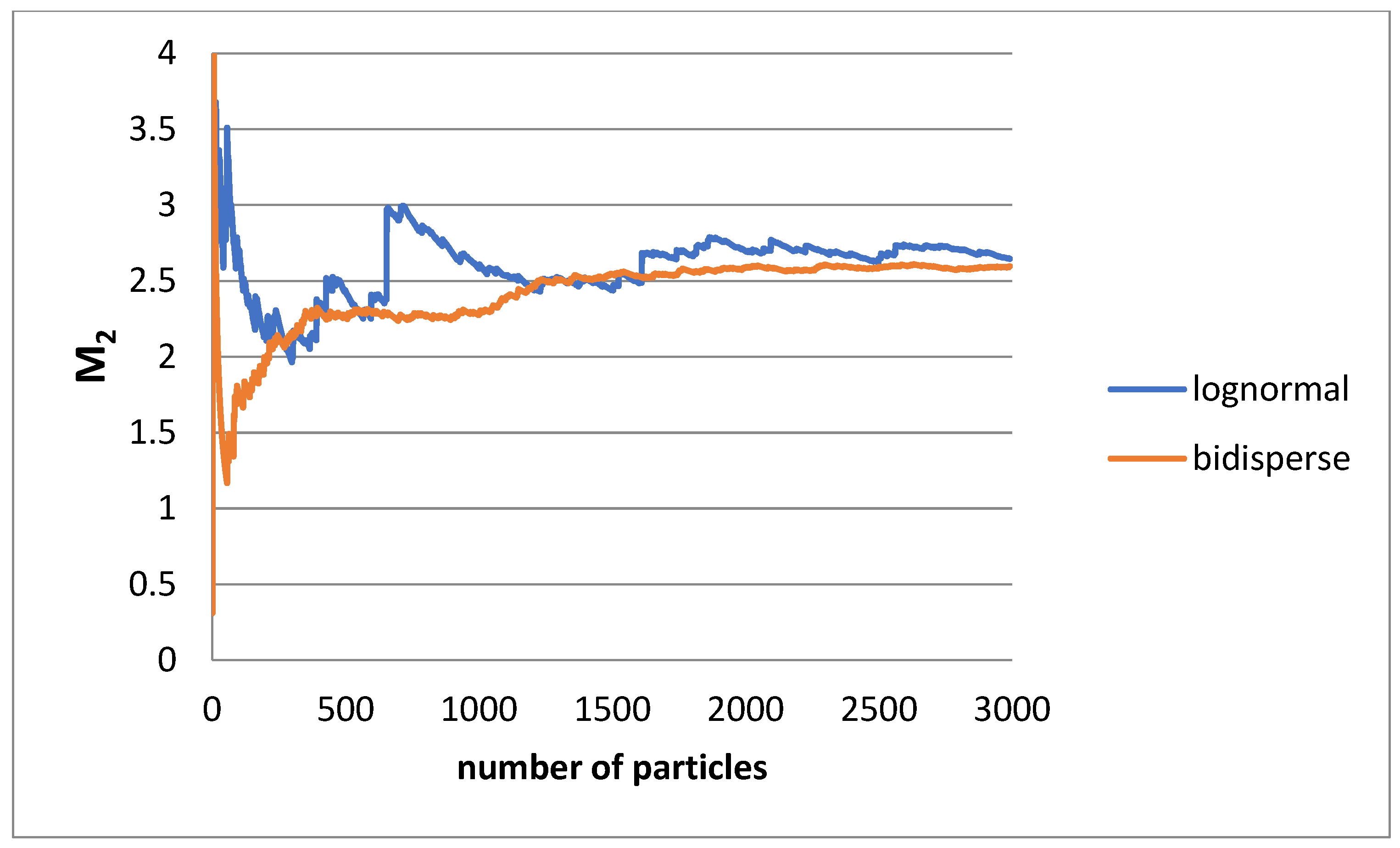
An important aspect of approximating the actual distribution with the bidisperse one is the smoother and faster convergence in the case of a Monte Carlo simulation. The unit problem must be solved several times (for instance, for a lognormal distribution) but only two times (for the two sizes) for the bidisperse distribution. In addition, the convergence for the bidisperse distribution occurs faster. This can be crucial in cases where complex calculations are needed (e.g., light scattering, diffusing wave spectroscopy [17,18]. It is well known that the broader the distribution is, the larger the number of particles that must be considered [19,20]. As an example, the computed normalized second moment of the distribution using a Monte Carlo method is presented in Figure 13 for a lognormal distribution with s = 1 and the corresponding bidisperse distribution versus the computational particles number. Pseudorandom numbers are generated using as a probability density function the lognormal and its bidisperse approximation, respectively, and the normalized second moments are calculated. The smoother behavior of the bidisperse case is evident. There are spikes in cases of lognormal distribution due to the finite possibility of introducing very large particles into the system. So, it is convenient to perform the Monte Carlo simulation (as long as moments with an order no higher than two are engaged in the computation) by using the bidisperse analog of the actual particle size distribution.

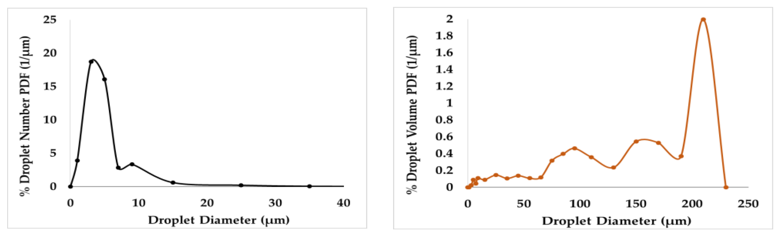
While the bidisperse approximation can be used to approximate any kind of particle size distribution, it is ideally suited for the case of a bimodal one. It is quite difficult to define what a bimodal distribution is. The existence of two peaks is a rather restrictive factor. It is believed that the more accurate feature of the bimodal distribution is the quite different range between the number-based and the volume-based distributions. As an example, the two forms of the probability density function (number and volume) for a dispersion of MCT oil taken in our laboratory (through image processing) appear in Figure 14. The bidisperse approximation analysis leads to small and large particle diameters of 5.3 and 128 μm, respectively, with number fractions of small and large sizes of 0.99 and 0.01, respectively. The employed matching moments are i = 0, 1/3, 2/3, and 1. The example, of course, is not based on the specific optimized recipe of the present work; however, it is a good description of the bidisperse approximation in practice.

5. Conclusions

It appears that for computational reasons, it is very convenient to replace a relatively broad actual measure of the particle size distribution with a bidisperse one. The approximation of the actual distribution according to the bidisperse one must be conducted in terms of moments in a finite region of orders. The best choice for the matching moments is to divide the region of moment order to three equal size intervals. However, this is not always possible because some moment orders are imposed by the physics of the problem. In this case, a hybrid approach of matching some moments and minimizing a global measure of deviation between moments of the distribution is proposed. It was shown that the approach works well for lognormal distribution up to dispersivity equal to three and for a moment order from one to two. In the case of unimodal distributions, the bidisperse approximation can be found analytically from Equations (20)–(22) and (9)–(13). In case of arbitrary distributions, the Equations (9)–(13) can be employed with numerically computed M₂ in place of e^s, and Equation (18) must be minimized with numerically computed moments of the distribution M_i. The proposed technique will be applied to proper parameterizing size distributions of emulsions taken in the laboratory.

References

- Hiemenz, P.C.; Rajagopalan, R. Principles of Colloids and Surface Chemistry; CRC Press: New York, NY, USA, 1997. [Google Scholar]
- Friedlander, S.K. Smoke, Dust and Haze. Fundamentals of Aerosol Dynamics; Oxford University Press: New York, NY, USA, 2000. [Google Scholar]
- Randolph, A.D.; Larson, M.A. Theory of Particulate Processes: Analysis and Techniques of Continuous Crystallization; Academic Press: London, UK, 1971. [Google Scholar]
- Flory, P.J. Principles of Polymer Chemistry; Cornell University Press: New York, NY, USA, 1953. [Google Scholar]
- Solsvik, J.; Jakobsen, H.A. Solution of the dynamic population balance equation describing breakage–coalescence systems in agitated vessels: The least-squares method. Can. J. Chem. Eng. 2014, 92, 266–287. [Google Scholar] [CrossRef]
- Lyklema, J. Fundamentals of Interface and Colloid Science Volume V: Soft Colloids; Academic Press: London, UK, 2005. [Google Scholar]
- Lakatos, B.G.; Sapundzhiev, T.J.; Garside, J. Stability and dynamics of isothermal CMSMPR crystallizers. Chem. Eng. Sci. 2007, 62, 4348–4364. [Google Scholar] [CrossRef]
- Williams, M.M.R.; Loyalka, S.K. Aerosol Science, Theory and Practice; Pergamon Press: Oxford, UK, 1991. [Google Scholar]
- Kostoglou, M.; Karabelas, A.J. Comprehensive modeling of precipitation and fouling in turbulent pipe flow. Ind. Eng. Chem. Res. 1998, 37, 1536–1550. [Google Scholar] [CrossRef]
- Kostoglou, M.; Karabelas, A.J. Modeling scale formation in flat-sheet membrane modules during water desalination. AIChE J. 2013, 59, 2917–2927. [Google Scholar] [CrossRef]
- Lee, K.W. Conservation of particle size distribution parameters during Brownian coagulation. J. Colloid Interface Sci. 1985, 108, 199–206. [Google Scholar] [CrossRef]
- Williams, M.M.R. On the modified gamma distribution for representing the size spectra of coagulating aerosol particles. J. Colloid Interface Sci. 1985, 103, 516–527. [Google Scholar] [CrossRef]
- Kostoglou, M.; Karabelas, A.J. An assessment of low order methods for solving the breakage equation. Powder Technol. 2002, 127, 116–127. [Google Scholar] [CrossRef]
- McGraw, R. Description of atmospheric aerosol dynamics by the quadrature method of moments. Aerosol Sci. Technol. 1997, 27, 255–265. [Google Scholar] [CrossRef]
- Singh, D.K.; Brito-Parada, P.R.; Bhutani, G. An open-source computational framework for the solution of the bivariate population balance equation. Comput. Chem. Eng. 2022, 161, 107780. [Google Scholar] [CrossRef]
- Press, W.; Flannery, B.; Teukolski, S.; Vetterling, W. Numerical Recipes: The Art of Scientific Computing; Cambridge University Press: New York, NY, USA, 1986. [Google Scholar]
- Lorusso, V.; Orsi, D.; Salerni, F.; Liggieri, L.; Ravera, F.; McMillin, R.; Ferri, J.; Cristofolini, L. Recent developments in emulsion characterization: Diffusing Wave Spectroscopy beyond average values. Adv. Colloid Interface Sci. 2021, 288, 102341. [Google Scholar] [CrossRef] [PubMed]
- Salerni, F.; Orsi, D.; Santini, E.; Liggieri, L.; Ravera, F.; Cristofolini, L. Diffusing wave spectroscopy for investigating emulsions: II. Characterization of a paradigmatic oil-in-water emulsion. Colloids Surf. A Physicochem. Eng. Asp. 2019, 580, 123724. [Google Scholar] [CrossRef]
- Caserta, S.; Simeone, M.; Guido, S. Evolution of drop size distribution of polymer blends under shear flow by optical sectioning. Rheol. Acta 2004, 43, 491–501. [Google Scholar] [CrossRef]
- Caserta, S.; Simeone, M.; Guido, S. A parameter investigation of shear-induced coalescence in semidilute PIB-PDMS polymer blends: Effects of shear rate, shear stress volume fraction and viscosity. Rheol. Acta 2006, 45, 505–512. [Google Scholar] [CrossRef]
Figure 1.
Ratio Ei of approximate to exact moment of order i for several values of lognormal distribution dispersivity s (Case 1).
Figure 2.
Ratio Ei of approximate to exact moment of order i = 0.6 and i = 1.5 for lognormal distribution dispersivity s (Case 1).
Figure 3.
Ratio Ei of approximate to exact moment of order i for several values of lognormal distribution dispersivity s (Case 2).
Figure 4.
Integrals P, P1, and P2 versus lognormal distribution dispersivity s (Case 1).
Figure 5.
Ratio Ei of approximate to exact moment of order i for several values of lognormal distribution dispersivity s (Case 3).
Figure 6.
Integrals P, P1, and P2 versus lognormal distribution dispersivity s (Case 3).
Figure 7.
Integral P versus small size of the bidisperse distribution η1 (Case 4).
Figure 8.
Ratio Ei of approximate to exact moment of order i for two values of the small size of the bidisperse distribution η1.
Figure 9.
Ratio Ei of approximate to exact moment of order i for several values of lognormal distribution dispersivity s (Case 4).
Figure 10.
Small size of the bidisperse distribution η1 versus lognormal distribution dispersivity s.
Figure 11.
Large size of the bidisperse distribution η2 versus lognormal distribution dispersivity s.
Figure 12.
Weight w1 of the bidisperse distribution versus lognormal distribution dispersivity s.
Figure 13.
Convergence of the second moment through Monte Carlo simulation using the lognormal and the corresponding bidisperse distributions (s = 1).
Figure 14.
Number and volume probability density functions of droplet diameter for a liquid–liquid dispersion.
Disclaimer/Publisher’s Note: The statements, opinions and data contained in all publications are solely those of the individual author(s) and contributor(s) and not of MDPI and/or the editor(s). MDPI and/or the editor(s) disclaim responsibility for any injury to people or property resulting from any ideas, methods, instructions or products referred to in the content. |
© 2024 by the authors. Licensee MDPI, Basel, Switzerland. This article is an open access article distributed under the terms and conditions of the Creative Commons Attribution (CC BY) license (https://creativecommons.org/licenses/by/4.0/).
Share and Cite
MDPI and ACS Style
Kostoglou, M.; Karapantsios, T.D. Approximation of Any Particle Size Distribution Employing a Bidisperse One Based on Moment Matching. Colloids Interfaces 2024, 8, 7. https://doi.org/10.3390/colloids8010007
AMA Style
Kostoglou M, Karapantsios TD. Approximation of Any Particle Size Distribution Employing a Bidisperse One Based on Moment Matching. Colloids and Interfaces. 2024; 8(1):7. https://doi.org/10.3390/colloids8010007
Chicago/Turabian StyleKostoglou, Margaritis, and Thodoris D. Karapantsios. 2024. "Approximation of Any Particle Size Distribution Employing a Bidisperse One Based on Moment Matching" Colloids and Interfaces 8, no. 1: 7. https://doi.org/10.3390/colloids8010007