1. Introduction
Structural analysis in aerospace, mechanical and civil fields often considers complex geometries with any kind of boundary and load conditions, materials and, in the case of multilayered structures, lamination sequences. These problems have the possibility to be solved by means of even more refined numerical models, whose target is to draw more and more precisely the behavior of the structure taken into consideration, emphasizing its salient characteristics, thus allowing a parallel decrease of the weights involved and an increase in safety. A certain degree of confidence is acquired by a numerical model once it has been deeply validated by means of an opportune juxtaposition with an exact 3D model [
1,
2]. Plates and shells are the common geometries used by these exact models because of their particular simplicity and specific load and boundary conditions. They allow the closed solution of the differential equilibrium equations that govern the phenomenon. The closed solution is essential in this validation process as it is the only way to obtain a punctual description of displacement, strain and stress fields without any numerically-related deviations. Several 3D solutions for plates and shells have been proposed in the literature; however, all of them are characterized by a dedicated solution for the specific geometry involved. The present 3D solution poses the problem in orthogonal mixed curvilinear coordinates, thus allowing a unique formulation for the equations of motion for rectangular and square plates, cylindrical and spherical panels and closed cylinders. No simplifications are introduced; the equations are written and solved in the most general case, the spherical panel, and they automatically degenerate into the ones for simpler configurations. The differential equations are solved using the exponential matrix method [
3,
4]. This approach needs constant coefficients. Several mathematical layers must be introduced in shell geometries to consider constant curvature-related terms.
Some of the most important 3D models proposed in the literature were developed for specific geometries. Pagano deeply analyzed the problem of the mechanical response of composite laminated structures. The cylindrical bending of composite laminated plates was studied in [
5] while an exact solution for rectangular and square, composite and sandwich plates was proposed in [
6], where the maximum stresses and deflections were investigated. More general load cases in cylindrical bending were considered in [
7]. Demasi [
8] found the exact three-dimensional solution for isotropic rectangular plates using the mixed form of Hooke’s law, and he showed the closed form expression for stresses and displacements of a rectangular plate under sinusoidal load. Fan and Ye [
9] analyzed the statics and the dynamics of plates with orthotropic layers overcoming the problem of increasing the number of equations to be solved with the number of the layers. Actually, the free vibration analysis of multilayered plates was proposed by several authors. Srinivas et al. [
10] proposed a three-dimensional solution for the free vibration of simply-supported, homogeneous and thick laminated rectangular plates made of isotropic materials. Circular and annular plates were studied by Taher et al. [
11]; the first frequencies were found for different thickness ratios and boundary conditions. Hosseini-Hashemi et al. [
12] used two different displacement fields to study the in-plane and the out-of-plane vibrations of a rectangular homogeneous plate, coated by a functionally graded layer. Messina [
13] used the exponential matrix method to solve the three-dimensional equations of equilibrium, written in a Cartesian coordinate system, for cross-ply laminated rectangular plates. The free vibration frequencies, stresses and deflections were presented. On the other side, Ye [
14] preferred to start from the recursive solution proposed in [
9] to study the free vibration of cross-ply plates. Other authors proposed different formulations valid for shells with an unavoidable increase in complexity with respect to the ones developed for flat cases. Varadan and Bhaskar [
15] studied the effects of harmonic loads applied to cross-ply cylinders; Fan and Zhang [
16] looked for an exact solution of the equations of elasticity in a curvilinear coordinate system. Also in these cases, several solutions have been proposed for the free vibration analysis. The free frequencies of simply supported composite mono and doubly-curved shells were found by Huang [
17] using the power series method. A further example for the use of the exponential matrix method to solve the 3D equilibrium equations may be found in [
18], where Soldatos and Ye wrote the equations in cylindrical coordinates, in order to calculate the free frequencies of angle-ply multilayered cylinders. Khalili et al. [
19] solved the free vibration problem for isotropic cylinders with different boundary conditions by means of the Galerkin method and writing the equations using the Hamilton’s principle.
Although several solutions were already proposed, all of them were written for a specific kind of geometry, with a lack of universality. In the present 3D solution, the equilibrium equations are written in orthogonal mixed curvilinear coordinates. The first author’s past works extensively described all the details of the proposed 3D formulation used for the free vibration analysis of one-layered and multilayered spherical, cylindrical and flat one-layered panels [
20,
21]. The same idea was extended to the static problem of shells subjected to harmonic loads on the top and bottom surfaces in [
22]. More general load combinations were considered in [
23]. In conclusion, this formulation can be used for the static and dynamic analysis of plates, cylinders and cylindrical/spherical shell panels. The method involves some parametric coefficients that depend on the radii of curvature and on the thickness coordinate
z. These coefficients allow the equations to degenerate into the ones for simpler geometries when one or both the radii of curvature are infinite. The exact/closed solution is obtained assuming a harmonic form for displacement components and loads, and considering the structure as simply supported. A simple stratagem of redoubling the number of variables allows the reduction to a system of first order partial differential equations. The exponential matrix method is then used to solve the reduced equation system across the thickness coordinate
z. In order to reach the solution, an opportune expansion order
N must be chosen for the exponential matrix. This method has constant coefficients for the first order partial differential equations in the plate case. When at least one radius of curvature is different from infinite, the parametric coefficients become functions of the thickness coordinate
z, and the coefficients for equations in each physical layer vary in
z. In these cases, several mathematical layers
M must be introduced to approximate the curvature terms and to solve the system. A convergence analysis for the introduced number
M of mathematical layers and for the order
N used in the expansion of the exponential matrix in the case of plates and shells (with different dimensions, thickness ratios, lamination sequences and geometries) is proposed in this paper. A similar study was already proposed for the free vibration analysis of sandwich and multilayered plates, cylinders and cylindrical/spherical shell panels in [
24] and for functionally graded plates and shells in [
25]. Theopportune combination of
M and
N values is essential in order to guarantee the convergence and to optimize the model in terms of convergence speed. As shown in [
25,
26], the use of mathematical layers is also useful when functionally graded materials are taken into consideration because it allows for better considering the evolution of the mechanical properties through the thickness.
2. Three-Dimensional Equilibrium Equations for Static Analysis
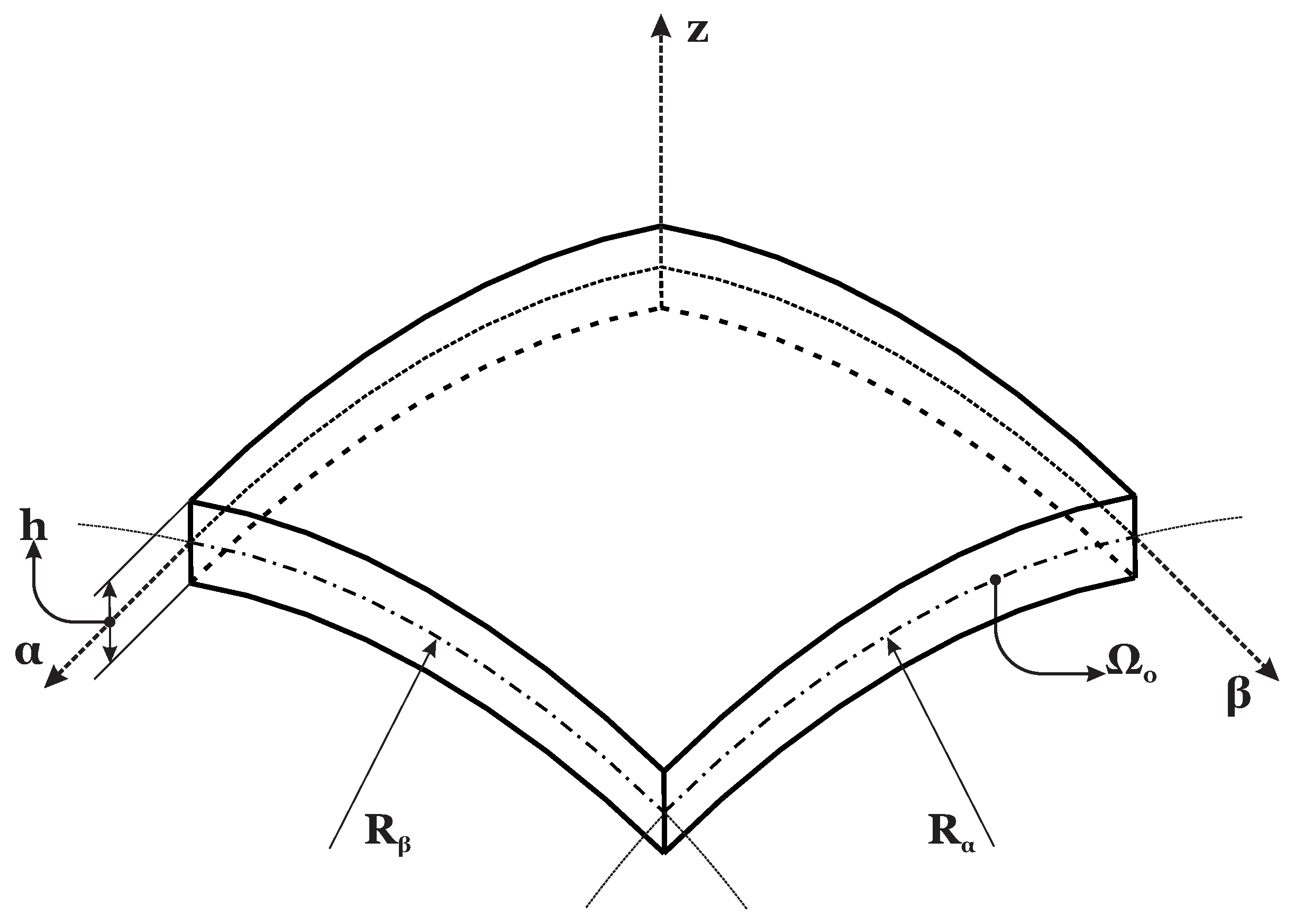
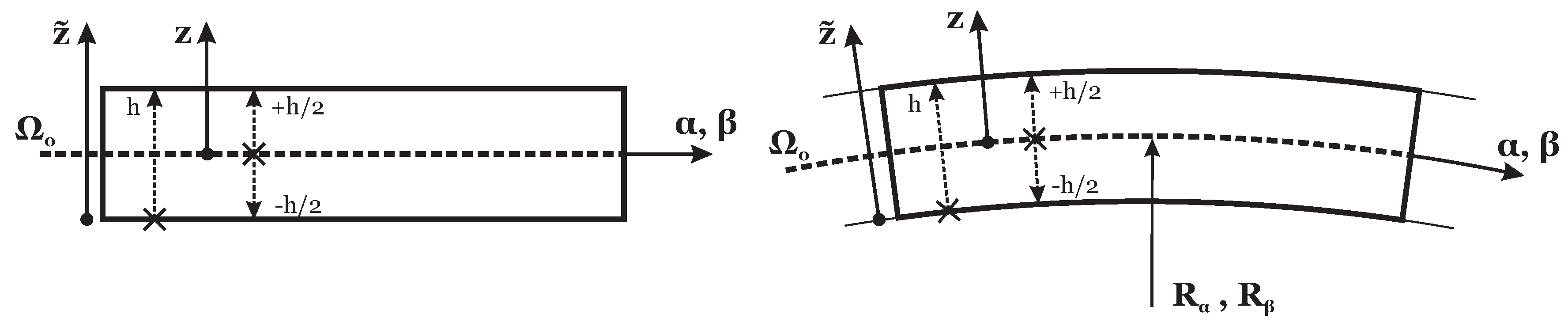
Notations, reference systems and geometrical parameters for shell structures in the most general case are indicated in
Figure 1 and
Figure 2.
is the middle surface of the shell, defined as the locus of points that fall midway between the bottom and the top surfaces. The reference system
is mixed curvilinear and orthogonal. Its origin is located in a corner.
z is normal to the middle surface, heading towards the upper surface.
and
lie on it.
h is the thickness of the shell,
z varies from –
h/2 to
h/2. For shells with constant radii of curvature in both directions, the following parametric quantities can be defined:
In Equation (
1),
and
are the radii of curvature referred to the mid-surface evaluated in
and
directions, respectively.
and
continuously vary across the thickness following the thickness coordinate
z or
.
Using the above coefficients, the static analysis of a spherical shell with a constant radii of curvature in
and
directions, made of a generic number
of layers, can be done writing for each
k layer the following differential equations of equilibrium:
k indicates the physical layer, so it may vary between 1 (at the bottom) and
(at the top); symbol ∂ stands for the partial derivatives. (
are the six stress components.
,
and
,
have been described before. A less specialized form of Equations (
2)–(
4), valid for shells with variable radii of curvature, may be found in [
2,
27]. In order to write Equations (
2)–(
4) in displacement form, the geometrical relationships and the constitutive equations must be introduced. A simplified expression of the geometrical relationships in orthogonal mixed curvilinear coordinates (see [
27,
28]) is possible when they are written for shells with constant radii of curvature. (
are the six strain components when the three displacement components
u,
v, and
w in direction
,
,
z, respectively, have been introduced:
The field covered by Equations (
5)–(
10) is wide. They are written for a generic spherical shell with constant radii of curvature. When one of the two radii of curvature
or
is infinite (
or
equal to 1), they automatically degenerate into equations for cylinders and cylindrical shells. When
(so
), they work for the plate case. The connection between the six stress components and the six strain components is obtained by means of the linear elastic constitutive equations. A closed form solution of Equations (
2)–(
4) is possible only considering orthotropic materials, with fibre orientation angle
equal to
or
in the structure reference system. These conditions lead to a simplified link between stress and strain vectors:
Details about the full version of the matrix of elastic coefficients may be found in [
29,
30].
For the closed solution of the Equations (
2)–(
4), a harmonic form for the three displacement components is assumed:
U,
V and
W, are the displacement amplitudes in
,
and
z directions, respectively.
a and
b are the shell dimensions, evaluated in the mid-surface
, in
and
directions, respectively.
p and
q are the half-wave numbers in the same directions. The coefficients of the two trigonometric functions are defined as
and
. Combining the constitutive Equation (
11) with the geometrical relations (
5)–(
10) and the harmonic form of the three displacements (
12)–(
14) into Equations (
2)–(
4), a displacement form of the equilibrium equations may be obtained in terms of the amplitudes of the displacements and their appropriate derivatives. Expressing in a compact form the partial derivatives
,
and
with the subscripts
,
and
, the differential equations of equilibrium in displacement form for a generic
n layer are:
As already seen for the geometrical relationships, the field covered by Equations (
15)–(
17) is wide because they are written for a generic spherical shell, but when one radius of curvature
or
is infinite (
or
equal to 1), they automatically degenerate into equations for cylinders and cylindrical shells. Likewise, when
(
), they work for the plate case.
The whole formulation that leads to Equations (
15)–(
17) takes into consideration the shell geometry via the parametric coefficients
and
, which depend on the thickness coordinate
z. As a result, the coefficients that multiply displacements and their derivatives in
z are not constant. Just in the plate case, as both the radii of curvature
and
are infinite and
, the coefficients of Equations (
15)–(
17) become constant and the exponential matrix method may be used directly to solve the system. In order to calculate
and
, each physical layer
k is divided in a certain number
M of mathematical layers
j. This makes the structure being constituted by
layers, where total index may be expressed by
. The coefficients are thus constant as they are evaluated with
and
measured on the mid-surface of the whole shell
, and
and
are calculated in the middle of each
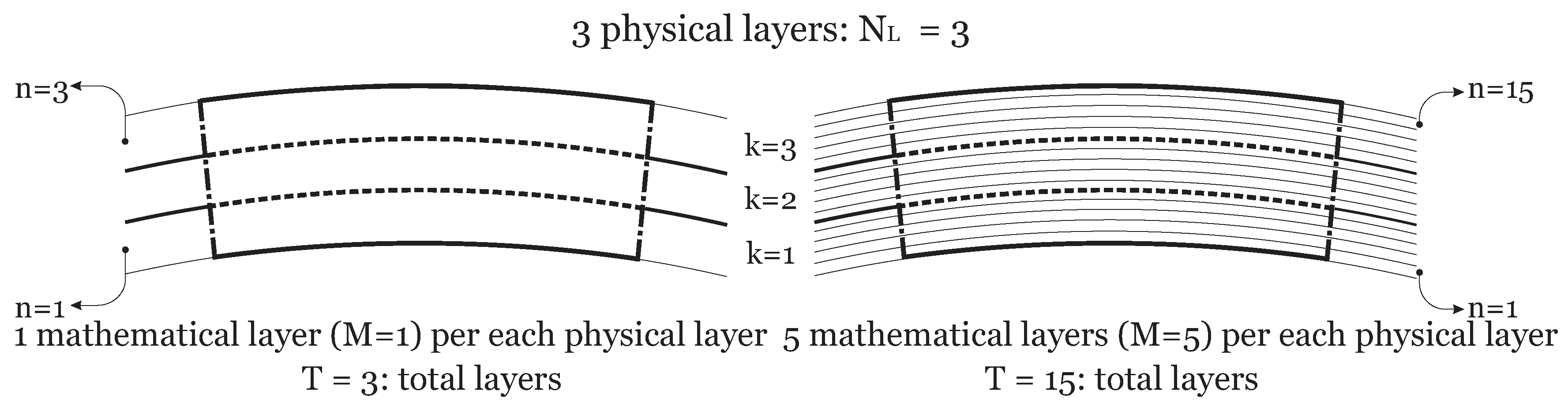
n layer. An example of the introduction of mathematical layers into the shell geometry is presented in
Figure 3, a three layered shell (three physical layers) is shown considering a number
M = 1 and
M = 5 of mathematical layers for each physical layer.
3. Use of the Exponential Matrix and Mathematical Layers in the Solution of 3D Equilibrium Equations
Assigning to each block in parentheses of Equations (
15)–(
17) a coefficient A
(with
s varying from 1 to 19), the system may compacted as:
These equations constitute a system of second order differential equations. A simple method of reducing its order to the first one is described in [
3,
31] and it may be summarized as a redoubling of the involved variables. In the first author’s past works [
20,
21], a detailed description of this approach can be found. The compact form of the reduced system of first order partial differential equations is:
where
and
. A further development of Equation (
21) is:
where
.
Equation (
22) is a system of first order differential equations that can be easily solved as shown in [
31,
32] with the exponential matrix method:
is the thickness coordinate of each mathematical layer and it varies from 0 at its bottom to
h at its top (see
Figure 2). The exponential matrix for each
n layer, with constant coefficients
A, is calculated with
=
h:
is the
identity matrix. The fast convergence ratio for increasing values of
N and its low computational time consumption were shown in [
4].
The relation in Equation (
23), evaluated at
, allows for linking the displacements (and their derivatives) within the bottom and the top of the same layer
n. The interlaminar continuity of displacements and transverse shear and normal stresses may be imposed at each interface. These quantities evaluated at the bottom of the
n layer must be the same as those evaluated at the top of the
layer:
Conditions in Equations (
25) and (
26) may be expressed via
transfer matrices
calculated for each interface. Details about their determination can be found in the first author’s past works [
20,
21,
22,
23,
24,
25,
26].
Plates and shells taken into consideration are supposed to have simply supported edges; moreover they can be loaded at the top (subscript
t) and/or at the bottom (subscript
b) of the whole laminated structure:
Grouping the loads applied on the bottom and the ones applied on the top in two separate vectors and specifying the stresses in terms of displacements and their derivatives, Equations (
29) and (
30), may be written as:
where
and
,
are
vector calculated at the bottom of the whole mutilayered structure (which means layer 1 and coordinate
), and at the top of the entire structure (which means layer
T and
).
Introducing recursively Equations (
25) and (
26) into Equation (
23), Equations (
31) and (
32) may be grouped into a general algebraic system:
with
.
Equation (
34) allows for finding the vector
, containing the values of the three displacement components and their respective derivatives at the bottom. The values assumed by vector
can be calculated at each value of the thickness coordinate
z by means of Equations (
23), (
25) and (
26). All of the details and the missing steps to reach the final solution may be found in the first author’s past works [
22,
33].
4. Results
The results presented in this section are given in order to find the best combination between the order of expansion
N of the exponential matrix
and the number
M of mathematical layers used to solve the differential equations written for shell geometries with assumed constant coefficients. Depending on the case, the structure may have a certain number of physical layers; each physical layer can be divided into
M mathematical layers, having the same thickness. An example on how a three-layered structure may be divided into a certain number of mathematical layers is presented in
Figure 3.
Results are presented in terms of no-dimensional displacements and/or stresses, with a specific factor for each case. When the present 3D solution converges, the results are indicated in bold. The cases presented hereinafter consider simply supported rectangular plates, cylindrical shell panels, cylinders and spherical shell panels. A summary of the loads, geometrical data and materials for the analyzed cases can be found in
Table 1 and
Table 2. All these geometries have been considered as multi-layered embedding a fibre reinforced composite material, whose properties are indicated in
Table 1. Different lamination sequences were considered, a symmetric cross ply laminate is taken into account in Cases 1, 3 and 4; an antisymmetric case is investigated in Case 2.
Case 1 was proposed by Pagano in [
6] for the exact 3D solution of a simply supported rectangular composite laminated plate. The material properties are indicated in
Table 1. The load, the geometry and the lamination scheme are indicated in the first column of
Table 2. Results are expressed in terms of no-dimensional displacements and stresses:
Case 2 was proposed by Ren in [
34] for the exact 3D solution of a simply supported composite laminated cylindrical panel. The dimensions, thickness values, load conditions and lamination scheme are proposed in the second column of
Table 2. Each layer has the elastic properties as proposed in
Table 1. Results are shown in terms of no-dimensional displacements and stresses:
Case 3 was investigated by Varadan and Bhaskar in [
15] for the exact 3D solution of a simply supported composite laminated cylinder. The in-plane dimensions, the considered thickness values, the mechanical load and the given values of half-wave numbers
are shown in the third column of
Table 2.
Table 1 shows the material properties. Results are calculated in terms of no-dimensional displacements and stresses:
The last considered geometry for the Case 4 was proposed by Fan and Zhang in [
35] for the exact 3D solution of a simply supported composite laminated spherical shell. The radii of curvature, the in-plane dimensions, the considered thickness values, the mechanical load and the half-wave numbers
are proposed in the fourth column of
Table 2 (see
Table 1 for elastic material properties). Results are expressed in terms of no-dimensional displacements:
Table 3 shows the displacement
and the stress
for the three-layered rectangular plate. Both of the quantities are given as dimensionless values and calculated in the middle. The displacement is evaluated for a plate whose thickness ratio is
, while the stress is for a structure with
. In this case, the introduction of
M mathematical layer is unnecessary. Actually, when
, the convergence is reached just by means of an opportune increase of the order of expansion
N. For the thinner plate,
is sufficient for the stress to reach the convergence; the thicker plate needs an higher value (
). The introduction of a certain number
M of mathematical layers helps to reduce the expansion order
N. However, for the computational point of view, the first procedure is more convenient. The comparison underlines the fact that an increase in
N value is needed as the thickness increases with respect to the shell dimensions. The convergence of the stress
with increasing values of
M is shown in
Figure 4 for several orders of expansion
N.
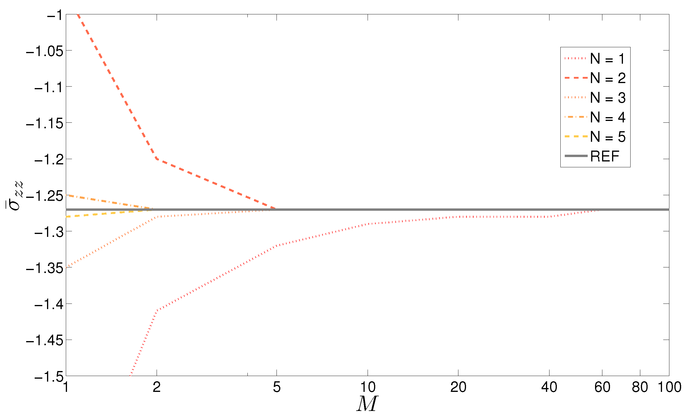
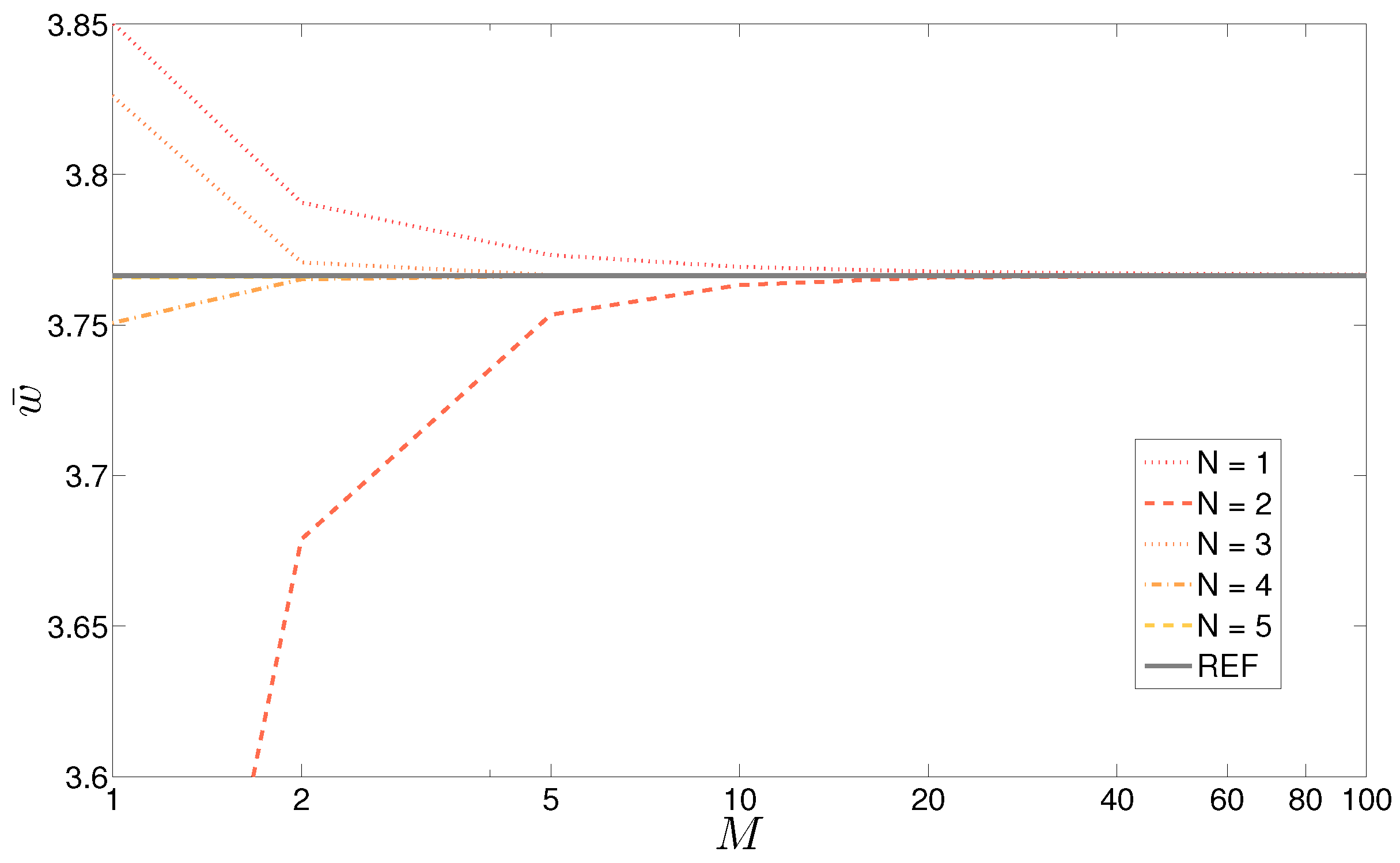
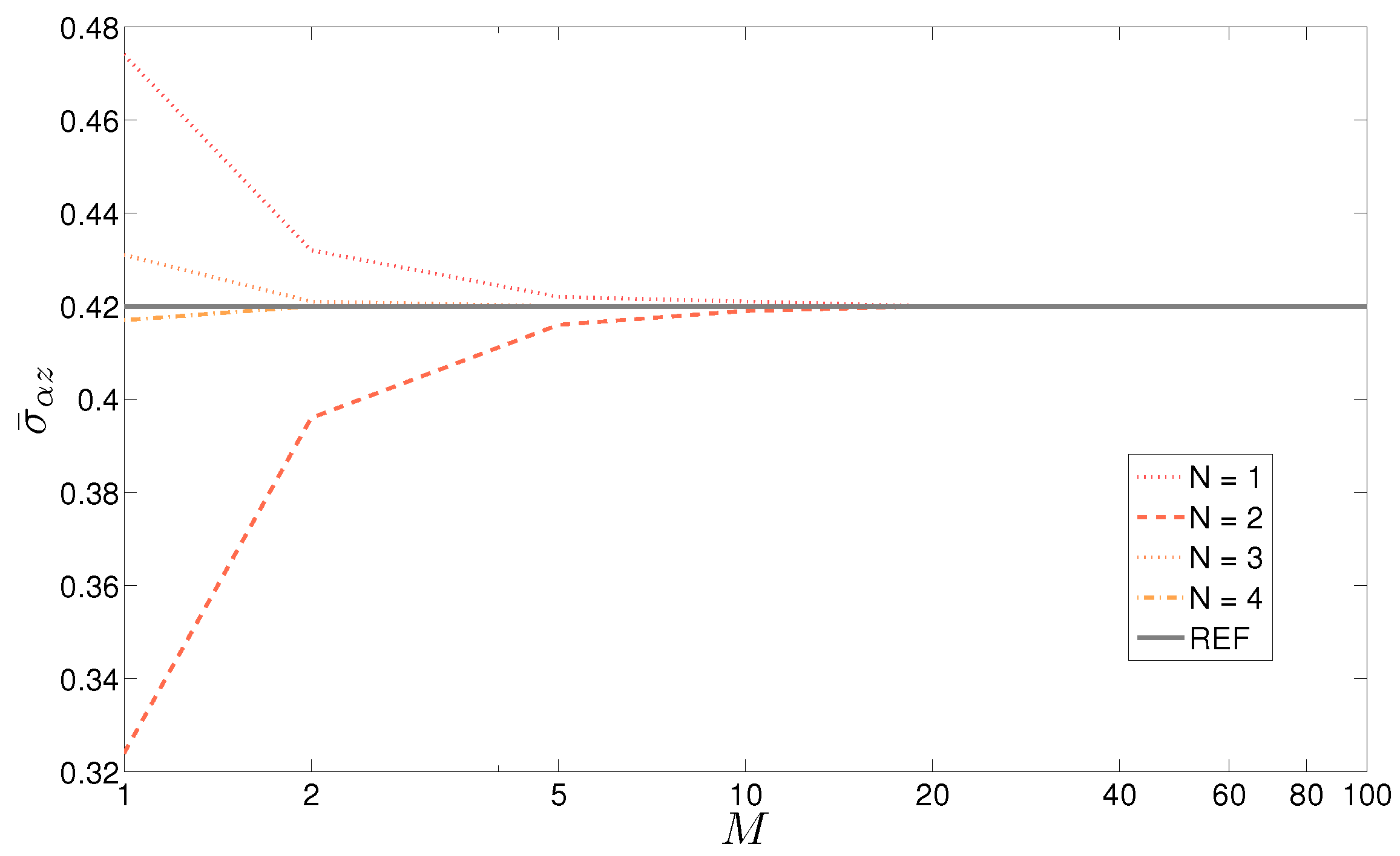
The displacement
and the stress
for the two layered cylindrical shell are shown in
Table 4. The displacement is considered in the middle, and the stress is on the top surface of the shell. A thick (
) and a moderately thick (
) panel are considered. All the values are given as dimensionless. This case remarks on the need for the introduction of mathematical layers when the curvature is introduced. In both cases, an increase in the order of expansion
N of the exponential matrix until 12 is totally ineffective until
mathematical layers are introduced into each physical layer. Under these circumstances,
is then sufficient to get the exact result for both moderately thick and thick shells. Convergence speed seems to be the same for different thickness ratios, while a slower convergence would have been expected for the thicker shell. This effect is tempered by the fact that the comparison is made on two heterogeneous quantities. As the displacements are a direct output of this formulation, they would generally converge faster than the stresses, which come from a combination of displacements and their derivatives. The results presented in
Table 4 are shown in
Figure 5 for the stress
with a progressive increase of the order of expansion for the exponential matrix until
.
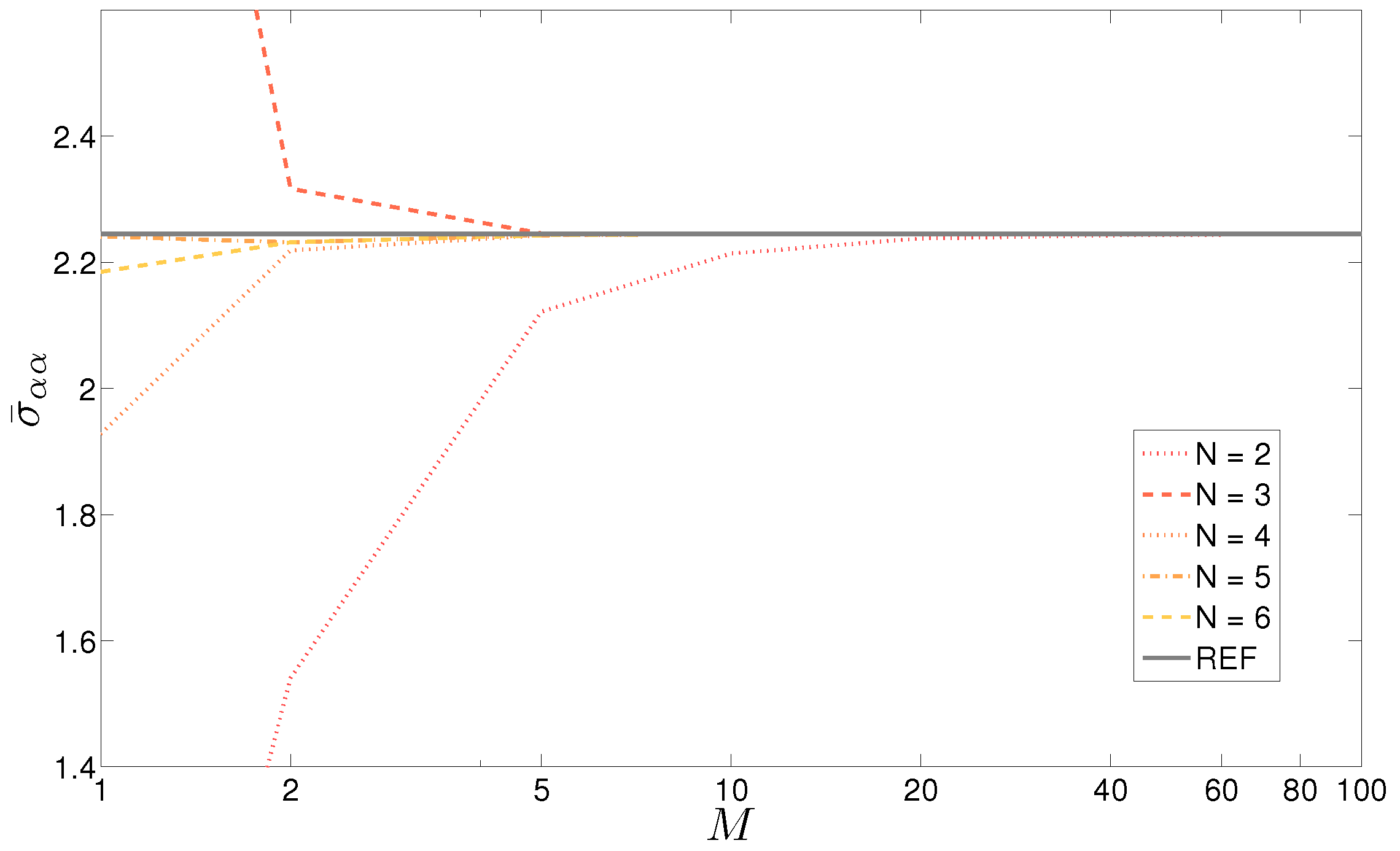
The results presented in
Table 5 are quite interesting. The considered case is the three-layered cylinder, with two different thickness ratios, which are
and
. The dimensionless displacement
and stress
are considered in the middle. These results show a faster convergence than that seen for the cylindrical panel. The moderately thick shell does not need the mathematical layers to be introduced, being convergent with just an expansion order of
. At the same time, the solution for the thick cylinder converges with just
mathematical layers coupled with an expansion order equal to
. On the contrary, the cylindrical panel needed
mathematical layers coupled with
for the displacement and the stress to be convergent. For these effects, an important role is played by the symmetry of the cylinder geometry and its related bigger rigidity due to the closed geometrical form. The effect of the thickness in the convergence speed is clear in this case despite the fact that heterogeneous quantities are investigated. Some of the results of
Table 5 are also shown in
Figure 6 for the thinner shell. The curves were drawn for different and increasing values of order of expansion
N.
Table 6 is for the last case about a three-layered spherical shell. Only the displacement
is investigated. The dimensionless values are given for a thick (
) and for a thin (
) structure. An increase in the expansion order of the exponential matrix is not sufficient without the introduction of a certain number of mathematical layers. As the investigated quantity is the same in both cases (the displacement), this study easily investigates the effect of the thickness. The coupled values of
M and
N needed to obtain a better description of the phenomenon increase with the thickness. When the thickness is small (compared to the shell dimensions),
mathematical layers coupled with
allows for the solution to be reached. On the other side, the thicker shell needs at least
mathematical layers with an expansion of the exponential matrix equals
.
Figure 7 confirms the trend shown in
Table 6 for the displacement
of the thinner shell: the results move close to the exact value as the order of expansion is increased.


