Article

Harnessing the Power of Remote Sensing and Unmanned Aerial Vehicles: A Comparative Analysis for Soil Loss Estimation on the Loess Plateau

by
Narges Kariminejad
1,
Mohammad Kazemi Garajeh
2,
Mohsen Hosseinalizadeh
3,
Foroogh Golkar
4 and
Hamid Reza Pourghasemi
5,*
1
Department of Natural Resources and Environmental Engineering, College of Agriculture, Shiraz University, Shiraz 71441-13131, Iran
2
Department of Civil, Constructional and Environmental Engineering, Sapienza University of Rome, 00138 Rome, Italy
3
Department of Arid Zone Management, Gorgan University of Agricultural Sciences and Natural Resources, Gorgan 49138-15739, Iran
4
Department of Water Engineering & Oceanic and Atmospheric Research Center, College of Agriculture, Shiraz University, Shiraz 71441-13131, Iran
5
Department of Soil Science, College of Agriculture, Shiraz University, Shiraz 71441-13131, Iran
*
Author to whom correspondence should be addressed.
Drones 2023, 7(11), 659; https://doi.org/10.3390/drones7110659
Submission received: 3 October 2023 / Revised: 29 October 2023 / Accepted: 30 October 2023 / Published: 4 November 2023
(This article belongs to the Topic Advances in Earth Observation and Geosciences)

Abstract

:
This study explored the innovative use of multiple remote sensing satellites and unmanned aerial vehicles to calculate soil losses in the Loess Plateau of Iran. This finding emphasized the importance of using advanced technologies to develop accurate and efficient soil erosion assessment techniques. Accordingly, this study developed an approach to compare sinkholes and gully heads in hilly regions on the Loess Plateau of northeast Iran using convolutional neural network (CNN or ConvNet). This method involved coupling data from UAV, Sentinel-2, and SPOT-6 satellite data. The soil erosion computed using UAV data showed AUC values of 0.9247 and 0.9189 for the gully head and the sinkhole, respectively. The use of SPOT-6 data in gully head and sinkhole computations showed AUC values of 0.9105 and 0.9123, respectively. The AUC values were 0.8978 and 0.9001 for the gully head and the sinkhole using Sentinel-2, respectively. Comparison of the results from the calculated UAV, SPOT-6, and Sentinel-2 data showed that the UAV had the highest accuracy for calculating sinkhole and gully head soil features, although Sentinel-2 and SPOT-6 showed good results. Overall, the combination of multiple remote sensing satellites and UAVs offers improved accuracy, timeliness, cost effectiveness, accessibility, and long-term monitoring capabilities, making it a powerful approach for calculating soil loss in the Loess Plateau of Iran.

1. Introduction

Spatial and temporal data drawn from global quantitative research have shown that erosion rates are much higher than soil production rates [1]. Soil nutrients discharge faster during soil erosion (SE) than they form, which threatens the sustainability of agroecosystems [2]. SE has been happening for hundreds of years, allowing the soil regeneration and regaining of its nutritional value. Additionally, it increases sediment transport (estimated to be 2.3 ± 0.6 BMT of sediment every year) beyond agricultural fields [3]. Due to climate change and land use changes, many areas are at risk of SE worldwide, including arid and semi-arid regions as well as humid ones [4,5]. Therefore, it is essential to detect and monitor soil loss in susceptible regions in order to ensure human health.
Space-born remote sensing images are most frequently used to obtain features of erosion on large scales with coarse spatial resolution [6,7,8,9]. However, some soil landforms (erosion features) are not as large as others; therefore, they are high-resolution remote sensing images [10,11]. During the last few decades, high-resolution and fine-grained data using unmanned aerial vehicle (UAV) images have become on-demand from low-altitude airspaces and are rarely distributed in developing countries [12]. Additionally, data from these soil landforms (e.g., sinkholes) are not publicly available in developing countries [13]. Therefore, different methods must be tested to derive spatial information regarding the erosional features, including sinkholes and gully heads.
As a result of increased data availability and thus a deeper knowledge of SE mechanisms, prediction equations have been developed based on some indicators such as soil properties, climate, vegetation cover, and topography [14,15]. Several mathematical and geospatial models (e.g., Revised Universal Soil Loss Equation-RUSLE) have also been proposed to forecast SE distribution at various temporal and spatial resolutions [16,17,18]. However, some uncertainties in outputs have resulted from nonlinear relationships between driving factors and related erosion processes, as well as the difficulty of upscaling the model results from a local scale to a larger scale [19]. Recently, data-driven machine learning methods have been increasingly applied to analyze the spatial distribution of SE [20,21]. In areas without observed field data, numerical models based on computational intelligence can provide probability-based distribution of erosion. These models are based on developing mathematical patterns between erodible areas and other properties [22]. Deep learning is the most effective machine learning approach and has attracted significant research attention [23,24,25,26]. Recently, the CNN method has been widely used to obtain more accurate earth feature mapping and modelling [27]. It can handle complex modeling well and use a large number of resources for training [28,29]. In the domain of deep learning data-driven networks, there is a regression relationship between input and output variables, which involves neurons [29]. The weights for the inputs from the first layer to the other layer are generated based on the connections between neurons. The weighted inputs are then adopted to produce a reliable output using a bias term [30]. To generate a desirable output, an activation function is applied to the neurons [31].
Several studies have resulted in fast and accurate outputs when using UAV for erosional feature modeling and mapping in remote and complex regions [32,33,34,35,36,37,38,39]. Although UAV data have recently been used to calculate erosional landforms [8,40], these studies calculated soil losses using three different images. In other words, this study proposed a novel deep-learning approach for calculating soil loss in the Loess Plateau of Iran, where a convolutional neural network was employed for the task of interest. In the proposed method, data from UAV, Sentinel-2, and SPOT-6 satellites were employed for model development and validation. Furthermore, this study intended to expand on previous research [24] and test the issues as follows: (1) a UAV image was applied to prepare high-resolution data in the region of losses of the Plateau of Iran; (2) multi-sources of remote sensing data (SPOT-6 and Sentinel-2) were used in the same region to detect soil maps of susceptible landforms; (3) the maps prepared from UAV and two remote sensing data were studied and compared; (4) finally, we examined the efficiency of CNN for detecting and mapping soil landforms.

2. Materials and Methods
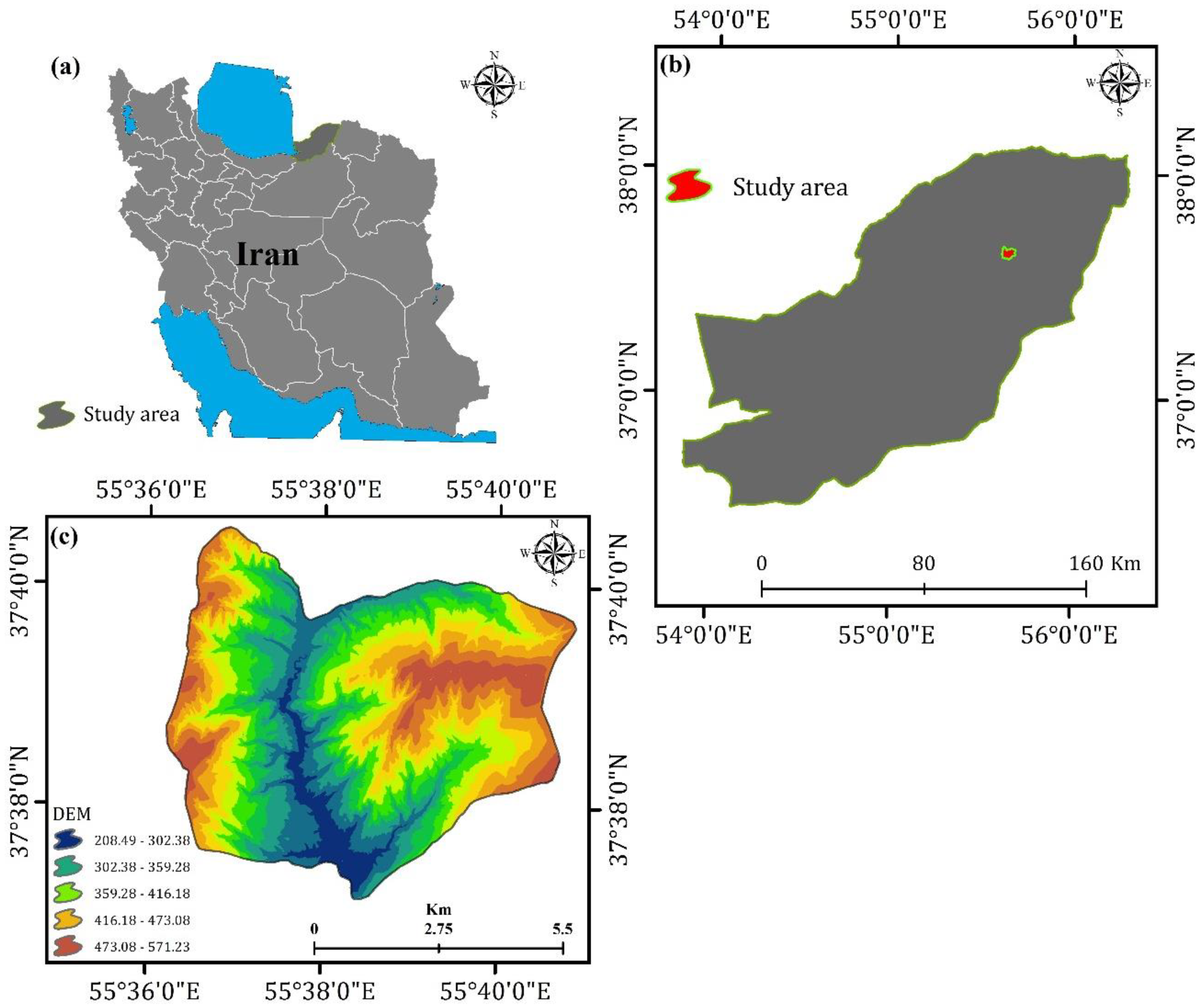
2.1. Study Region

The study area is located in northeast Iran (Golestan Province) (37°36′40″ N to 37°38′40″ N latitudes, and 55°39′40″ E to 50°41′40″ E longitudes), with approximately 500 hectares of a dominantly semi-arid climatic region. The study was conducted in loess-driven soils with a mean of 265 mm precipitation per year. The min and max altitudes are 210 m and 550 m above sea level (Figure 1), respectively, with the dominant “silt loam” texture of the soil surface and the whole region covered by loess soils.

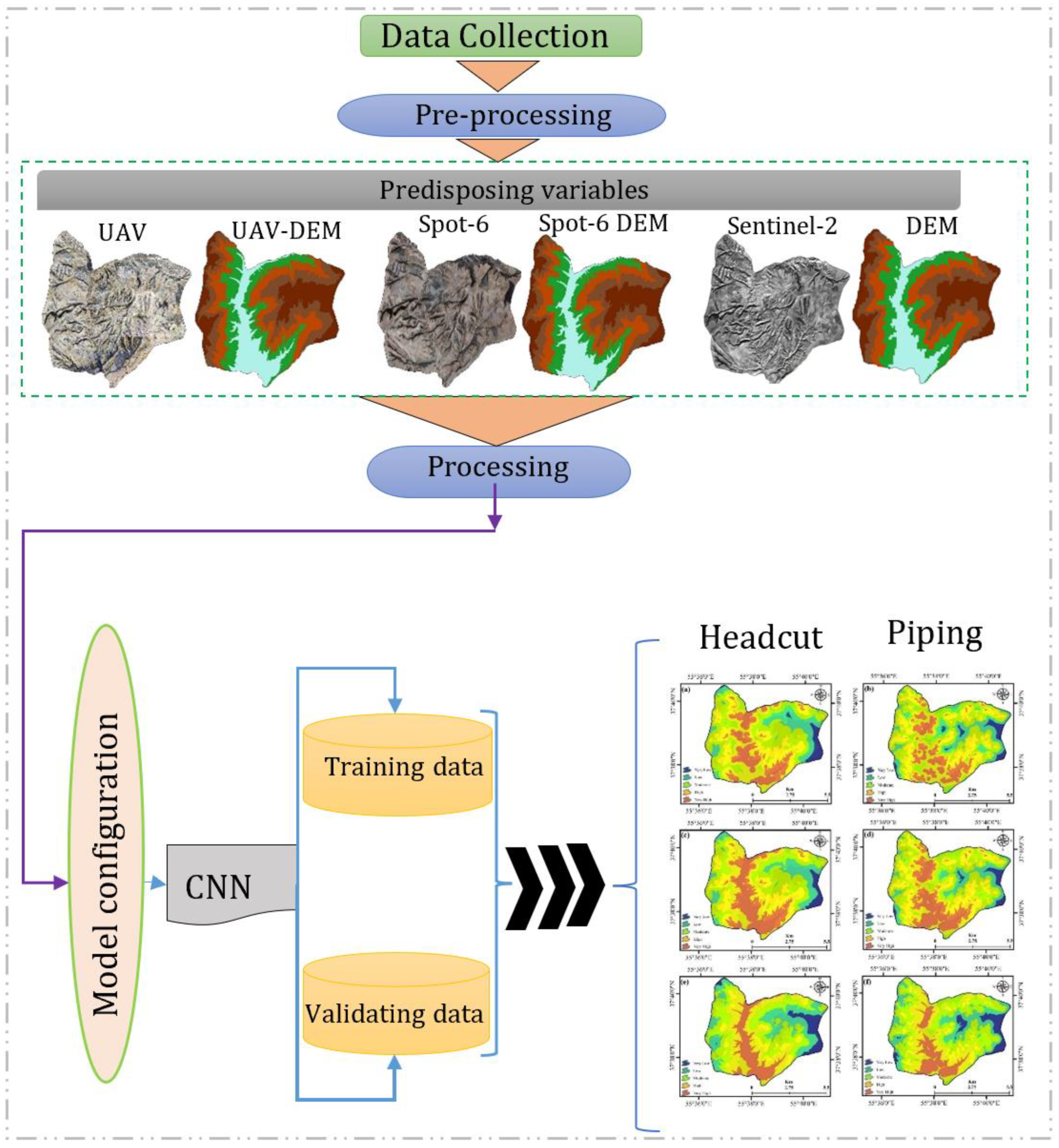
2.2. Flowchart and Framework of the Present Research

Information regarding the UAV and two remote sensing datasets (SPOT-6 and Sentinel-2) were prepared and applied in the present study. We collected the UAV, SPOT-6, and Sentinel-2 datasets on three different dates: 18 August 2019 for both the UAV and SPOT-6, and 14 September 2019 for Sentinel-2. The soil landforms (erosion features) in the loess region were computed by applying a deep learning model called CNN (Figure 2). The first step was to prepare, gather data sources, and digitize the location of two erosion features, including the sinkhole and the gully head. To this end, 48 ground control points, GCPs, were gathered from the study area: 70% of the data were allocated for the training section and 30% for testing the model. Elevation data and topographic information were collected using SPOT-6, Sentinel-2 remote sensing, and UAV images (Table 1). The next step involved image processing of the remote sensing and UAV data that were entered as the inputs of SE susceptibility maps. The images of the UAV with a pixel size of 0.2 m were processed using Pix4D software (Versions 3.3). The land surface/subsurface maps were processed in ArcGIS 10.8, and the main indices/factors were extracted from UAV-DEM. Next, susceptibility maps were computed and validated applying the CNN method. In the fourth step, erosional landform maps were prepared and validated using two remote sensing datasets named SPOT-6 and Sentinel-2. In the final step, we analyzed and compared the results calculated from the UAVs and two different remote sensing satellites (Figure 2).

2.3. The Preparation of the UAVs and Two Satellite Images

Soil erosional features, including sinkholes and the gully head, were calculated and detected using UAV data and remote sensing satellite images. Phantom 4RTK was equipped with a C4K camera, 1-inch CMOS sensor that can shoot 20MP photos and an 8-element lens with an 84-degree FOV. Video was recorded in H. 264 or H. 265 and C4K resolution of 4096 × 2160 up to 60 fps for excellent results. It had a 1/2.3-inch sensor that is comparable in size to that of a camera phone. The Phantom 4’s remote control and live feed are based on DJI Lightbridge technology, providing an effective control range of up to 3.1 mi (5 km) in unobstructed areas that are free from interference. At this stage, the digital model of the area’s height was prepared from the images and point clouds prepared by the UAV in pixels of 0.2 m. The images were taken in an area (2700 hectares) with a flight height of 200 m from the ground and a flight speed of 10 m per second with an overlap of the flight paths of 75%. The flight path was specified by the Pix4D software, and the bird moved automatically according to the defined air paths. After the flight operation, the processes included automatic internal, relative, and absolute justifications, which led to the preparation of point clouds of the area and a digital height model.
Before conducting aerial photography, BM stations and non-permanent signs of ground control points were designed, and their approximate locations were determined. Owing to the non-flatness of the area, BM points were positioned at intervals of at least 1 km using the Differential Global Positioning System (DGPS) method with a triple set of Global Navigation Satellite System (GNSS) receivers. The DGPS network was positioned with at least one reference point (mapping organization or the Shamim system). The marking of non-permanent ground control points was performed before the flight, and their quality was such that they could be seen and measured in all aerial images. The density of these signs can vary between 150 and 400 m depending on the presence or absence of the GNSS/Inertial Measurement unit (IMU) sensor, the flight height, and the quality of the images. Landmarks were located by Real Time Kinematic (RTK)-GNSS method from the nearest BM. One of the essential parts of a drone mapping project is flight and aerial imaging. Therefore, the proper functioning of the bird was ensured to have the correct flight and quality images, as well as to prevent all kinds of financial losses or even lives. In addition, before the flight operation, the parameters related to photography, including shutter speed, ISO (the sensitivity of the camera’s sensor), focus, and aperture, were adjusted to obtain high-quality images and proper lighting. Quality products were obtained during the processing stages.

2.4. Definition of CNN Method for Detecting Soil Erosional Features

To reduce land degradation and mitigate the adverse effects of erosion on ecosystem services, it is necessary to accurately predict SE susceptibility. Several theoretical and empirical models, including RUSLE (Revised Universal Soil Loss Equation), USLE (Universal Soil Loss Equation), WEPP (Water Erosion Prediction Project), SWAT (Soil and Water Assessment Tool), and WaTEM/SEDEM (Water and Tillage Erosion Model and Sediment Delivery Model), can be employed to study soil erosion [41,42]. In contrast to the traditional soil erosion modelling approach, which requires a physically or empirically based model for prediction and collection of field data to verify the accuracy of the model, a machine learning-based approach does not require prior modelling. Additionally, a new approach is essential to address the diverse factors influencing land degradation and soil erodibility [43]. Instead, field measurements are used directly to formulate rules and draw generalizations from the data, leading to predictions using semi-automated and automated approaches, such as learning-based techniques [44,45]. Deep learning, a subset of machine learning, has found practical applications in modeling and mapping various earth features. Among the prevalent deep learning techniques utilized for this purpose are Convolutional Neural Network (CNN), Recurrent Neural Network (RNN), Denoising Autoencoder (DAE), Deep Belief Network (DBN), and Long Short-Term Memory (LSTM) networks. Notably, CNN is a fully connected feedforward neural network celebrated for its ability to effectively reduce the number of parameters while preserving model quality compared to other deep learning methods [46]. This attribute is particularly advantageous when working with high-dimensional data, such as images, where each pixel serves as a feature, making it well-suited for harnessing the power of a CNN [47]. Utilizing CNN for soil erosion modeling can also lead to cost and time savings in preparation and classification processes. In recent years, several researchers have used the CNN model to accurately map the dynamic features of the Earth [40,48,49]. A CNN is a feed-forward type of neural network that utilizes convolutional calculation and a depth structure, which is a representative algorithm for depth learning. A CNN consists of a hidden layer and an input layer which can include a pooling layer, a convolution layer, a whole connection layer, and finally an output layer. The input layer comprises an m × n matrix with the respective feature value at each node. Our input layers for detecting soil erosional features were the DEM, satellite images, and training datasets. A convolutional layer immediately adjacent to the input layer is sometimes referred to as the feature extractor. This is because it is applied to extract the features of an image. Several convolutional kernels were used in the convolutional layer, which was optimized by a back-propagation algorithm. The input for the next layer is the output of the convolutional layer [50,51,52,53]. In general, six convolutional layers were used to detect soil erosional features (Table 2). We constructed CNN models with a two-layer depth for soil erosional features. This means that for each separated dataset (UAV, SPOT-6, and Sentinel-2), a two-layer depth consisting of DEM and satellite images was constructed for detecting the gully head and the sinkhole. Each two-layer depth CNN model was fed predisposing variables (DEM and satellite images). In this study, we applied multiple convolutions with different filters ( 2 × 2 ), resulting in feature maps. All the feature maps were then gathered, and the results of the convolutional layers were produced.
Each convolutional layer consists of a pooling layer, an activation function, and multiple weights [54]. A down-sampling algorithm is used in the pooling layer to reduce overfitting and minimize dimensionality [55]. Max pooling is employed as a maximum operator to down sample the feature maps in the encoder. The feature maps must be manipulated using maximum pooling “to split them into several rectangular regions” to generate maximum values for the regions. A fully connected layer is used to reduce the loss function and subsequently output classification results [56,57].
The previous convolutional layers must be weighed to construct a weighted sum. The weighted sum then passes through an activation function [58]. The ReLu (Rectified Linear Unit) was applied in the current study, which is defined according to Equation (1). In the field of deep learning, ReLu is very popular. The function considers negative values (below zero) as zero, positive values (greater than zero), and values equal to zero as its own. As its relationship is linear, it is faster than the sigmoid and Tanh functions owing to its computational efficiency.
f x = { 0 ,   x < 0   x ,   x 0 .
A back-propagation algorithm is then applied to optimize all parameters in a CNN model, which is applied to decrease the value of the loss function. The cross-entropy loss was used when adjusting the model weights during training. Therefore, the aim was to minimize the loss because the best model has a smaller loss. In general, a cross-entropy loss of zero considered a perfect model [30]. The optimizer was calculated as follows:
L y ,   y ^ = 1 N i = 1 N y i   l o g   l o g   y ^ i + 1 y i l o g   l o g   1 y ^ i ,
where N is the total number of obtained quantitative samples from the study area, y i is the natural result of sample i , y ^ i is the predicted likelihood of sample i , whose output is 1, and y and y i reveal the accurate output vectors and predicted probabilities, respectively.

2.5. Output Validation

The result’s classification validation is a critical phase in image analysis to complete a preliminary assessment of the structural model and conceptual framework [59,60,61]. This study utilized ROC curves to assess the accuracy of the flood models. In the ROC curve, there are two crucial axes: vertical and horizontal. The vertical axis corresponds to true positives (TP), indicating correctly labelled flood-affected pixels. Conversely, the horizontal axis represents false positives (FP), indicating incorrectly labelled flood-affected pixels. The Area Under the Curve (AUC) serves as a metric to quantify the accuracy of prediction model results [61]. The outputs of the accuracy assessment for detecting gully heads and sinkholes are represented in Table 3. According to Table 3, the CNN model performed well with an AUC of >0.89 for gully head and sinkhole detection, respectively.
We also applied loss, validation loss, accuracy, and validation accuracy in Python-based Spyder software (version 3.7) to estimate classification accuracy. Table 4 shows the results of the accuracy assessment using Python-based Spyder software.

3. Results and Discussion

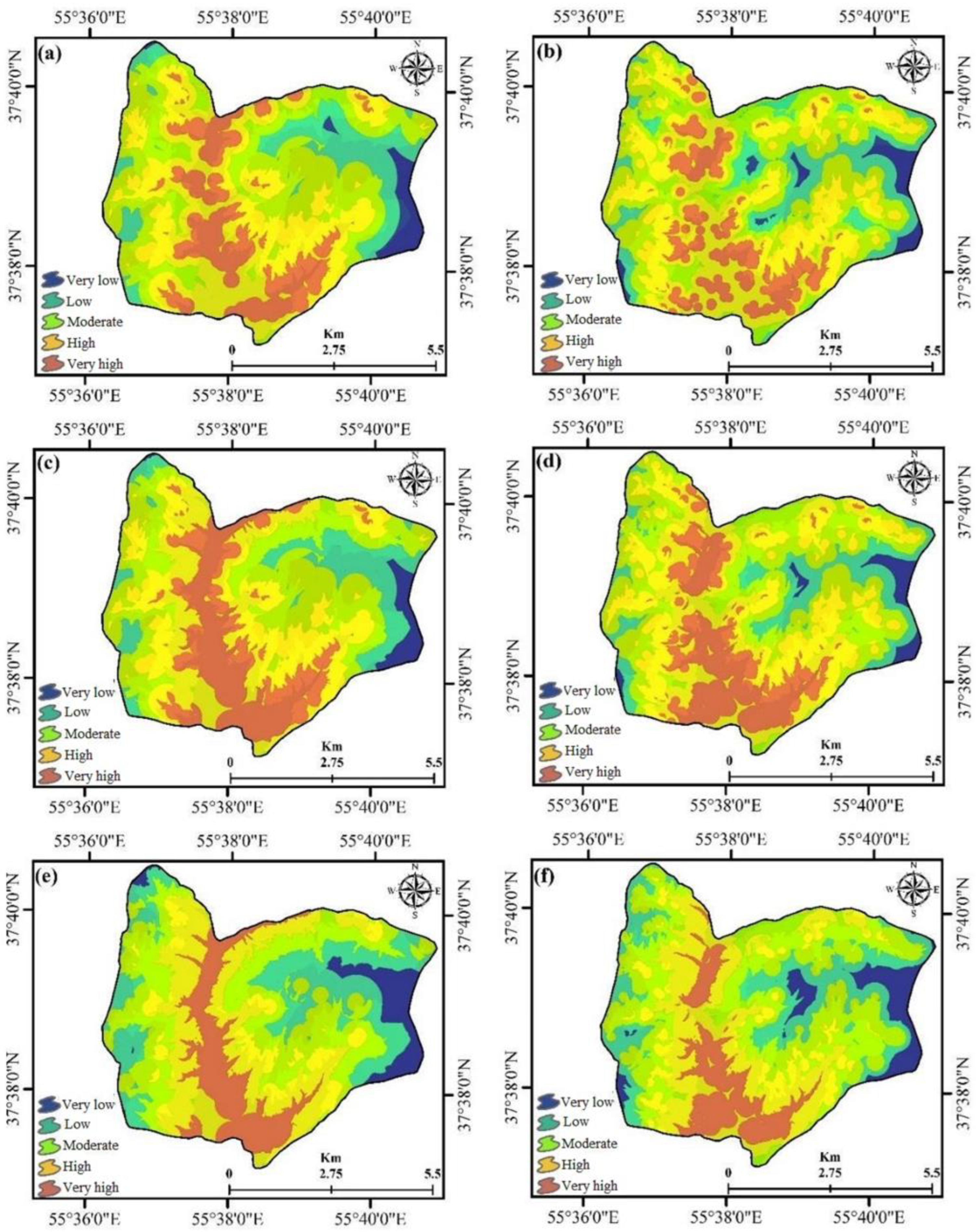
3.1. The Detected Maps of UAV, SPOT-6 and Sentinel-2 Using CNN Method

This study employed an automated CNN data-driven approach to compare the results of different UAV, SPOT-6, and Sentinel-2 images and their derived DEMs for detecting and mapping gully head and sinkhole. In other words, the main contribution of this work is the development of an approach using deep learning and convolutional neural networks (CNN) to compare and detect soil landforms, specifically sinkholes and gully heads, in hilly regions. For detecting erosional features, UAV, SPOT-6 and Sentinel-2 images with pixel sizes of 0.2, 6, and 10 m, respectively, were employed. ReLu, cross-entropy, and Adam were applied as activation, loss, and optimization functions for detecting the gully head and the sinkhole in the CNN models. In Figure 3, the CNN results for detecting soil erosion features are presented. Our results showed the highest performance of the CNN based on UAV datasets for detecting and mapping soil erosional features (Table 3). The results of this research show that the gully head was detected using CNN with an AUC of 0.9247, 0.91.05, and 0.89.78 for UAV, SPOT-6, and Sentinel-2, respectively (Table 3). Our findings also show that CNN performed well for detecting sinkholes with AUC of 0.9189, 0.9123, and 0.9001 for UAV, SPOT-6, and Sentinel-2, respectively (Table 3). To better understand the performance of the CNN, we employed four functions including loss, validation loss, accuracy, and validation accuracy in Python-based Spyder software, as shown in Table 4. According to Table 4, CNN performed well in gully head detection with accuracies of 0.9452, 0.9214, and 0.9012 for UAV, SPOT-6, and Sentinel-2, respectively. It also achieved accuracies of 0.9324, 0.9201, and 0.9135 in sinkhole detection for UAV, SPOT-6, and Sentinel-2, respectively, as shown in Table 4. The results of this study emphasize the dependency of soil erosional feature accuracy on the resolution and quality of DEM data. Overall, by combining the detected maps obtained from the UAV, SPOT-6, and Sentinel-2 imagery, we can create a comprehensive and multi-scale analysis of the study area. This integration offers a holistic view, capturing fine details from the UAV data, broader coverage from SPOT-6, and spectral richness from Sentinel-2. Such combined maps can provide valuable insights for diverse applications, enabling informed decision making and accurate assessment of the study area.

3.2. Disadvantages and Advantages of UAVs in Using the CNN Model

In this research, recently published findings [24] were extended to detect sinkhole collapses and gully heads using UAV, SPOT-6, and Sentinel-2. Because the pixel size of the satellite images was not at the same fine resolution as UAVs, it was difficult to obtain soil loss information continuously. Considering the importance of satellite data, data at various spatial or temporal resolutions can be used in environmental studies. However, these data should be compared and checked with the acceptable spatial resolution of UAV images, and the present study must study and assess this issue. However, this study showed that the UAV and two satellite images had acceptable accuracies. It is challenging to use satellite images in studies of soil loss size (i.e., volume, width, and height) [30]. Therefore, to ensure good results from different methods, especially to detect information regarding the size of erosional features, UAVs are much better than the others.
Elevation data obtained from UAVs remote sensing has various benefits, including the high spatial resolution of the region and its flexibility [21]. A very high resolution is an essential advantage of UAVs, and because of the low altitude of UAV flights, imaging problems from the atmosphere have decreased [32,62]. Therefore, highly accurate information regarding erosional landforms and elevation values can be easily generated from UAVs. In addition, UAV deployment has become critical in terms of accessibility. In developing countries, several data barriers and limitations, such as inaccessibility to high-resolution/up-to-date satellite imagery in areas prone to land degradation, have limited the wider dissemination of existing data sources, and there is a need to use other means, such as drone imagery. This has motivated the search for new techniques to obtain spatial information about erosional characteristics. It should be noted that land subsurface/surface information and much more quantitative data from more significant regions (i.e., studied on national scales) can be obtained from the SE sources gathered by remote sensing satellite images, including SPOT-6 and Sentinel-2. In addition, UAV-driven data are much more expensive; for instance, having soil loss data with satellite imagery data from 500 hectares is about one twentieth that of gathering UAV data in the same region size. The UAV also has more limitations. For instance, it is not feasible to obtain different hydro-geomorphologic variables (i.e., flow velocity, and water depth) from UAVs, although they can be easily obtained from satellite data [63,64]. In addition, UAV remote sensing has a restricted range, such as the possibility of flying, only in clear sky conditions. Moreover, as UAVs become more popular and demand for them increases, they become increasingly vulnerable to a number of security attacks [65]. Although the capabilities of drones will expand in the coming decades, social organizations and governments must be aware of the security aspects of drone communications [66]. Overall, although UAVs offer significant advantages in utilizing the CNN model for various applications, it is essential to consider the limitations of flight endurance, weather dependency, regulatory compliance, and data management. By addressing these challenges, UAVs can effectively enhance the performance of the CNN model and enable the accurate and timely analysis of high-resolution aerial imagery.

3.3. The Positive and Negative Points of Multiple Remote Sensing Sources in Using the CNN Method

Multiple sources of remote sensing have increased the usage of the “CNN” method. Other data from satellite images can be applied to detect soil losses [67]. In the current research, the two-satellite data were gathered at the time when we obtained UAVs in the fields, and it means that there were more data accessible to support the soil losses in the Loess Plateau of “Golestan” province. The SPOT-6 and the Sentinel-2 data were equally efficient for computing soil losses in the studied region. Then, they offered good results for spatially detecting erosional landforms. Therefore, we achieved well-calculated soil loss map (Figure 2) outputs from multiple satellite sources, both due to the spatial resolution and because erosional landforms in the region were very large for detection with different satellite images. Recently, we expanded the application of the CNN model by applying data from multiple satellite images.
We are aware that data from multiple satellite sources have excellent temporal resolution in contrast to UAVs. In future research, we must be able to combine much deeper learning methods with multiple satellite platforms on large scales. After the detection of soil loss, the changes in the dimensions of soil landforms can be monitored in the short-term. Long-time detection of other soil landforms, including gullies and mass movements, can be managed using UAV or data from multi-platform satellites, such as LiDAR [68], thermal infrared remote sensing [69], and optical remote sensing (e.g., Landsat [70]). Overall, the use of multiple remote sensing sources in conjunction with the CNN method offers great potential for improving performance and accuracy. However, it is important to be mindful of the challenges associated with data fusion and the computational requirements. With careful consideration and proper techniques, the benefits can outweigh the drawbacks, leading to a more accurate and detailed remote sensing analysis.

4. Conclusions

The research paper highlights the importance of using drones and satellite images to identify sinkholes and gully heads so that soil losses in the form of erosion can be calculated. In the present study, we applied UAV and multiplatform satellite-acquired data, such as SPOT-6 and Sentinel-2, to detect erosional landforms in the Loess Plateau of Iran. RC values obtained from the UAVs were 0.89 (sinkhole) and 0.88 (gully head), respectively. We then calculated the RC values of soil losses with the SPOT-6 data, which were 0.87 (gully head), and 0.86 (sinkhole). The RC values calculated with the Sentinel-2 were 0.86 (gully head), and 0.85 (sinkhole). The results showed the excellent performance of the proposed method, which can be considered a potential solution for practical use. However, to effectively manage SE, especially in erosion-susceptible soils, more hydro-geomorphological information is required over time. The UAVs prepared accurate information that was subsequently applied to compute soil losses. The UAVs offered very good results in detecting soil losses, although Sentinel-2 and SPOT-6 provided good results, too. The use of UAV images in SE mapping confirms some benefits in comparison to the sensing and orbital acquisition methods. Some characteristics such as flying in lower altitudes, less atmospheric interference, and, importantly, quite lesser expense are the benefits of this acquisition system in both scientific and commercial explorations. With the CNN method, the UAV and other satellite remote sensing data confirmed accurate values, and we believe that this model will be beneficial for SE research groups and managers worldwide. However, it is recognized that one of the significant motivations behind CNN popularity these days is the large amount of accessible data to acquire knowledge. The basis is a CNN which uses images as inputs and provides a feature map that illustrates the image with semantic features. Future research on geospatial–temporal hazard analysis should be considered using other deep learning models for satellite imagery.

Author Contributions

Conceptualization, N.K.; methodology, M.K.G.; software, M.K.G.; validation, N.K.; formal analysis, M.H.; investigation, N.K.; resources, N.K.; data curation, M.H.; writing—original draft preparation, N.K.; writing—review and editing, H.R.P.; visualization, F.G.; supervision, H.R.P.; project administration, H.R.P. All authors have read and agreed to the published version of the manuscript.

Funding

This work was supported by the College of Agriculture, Shiraz University (Grant No. IGRC1M27143).

Data Availability Statement

Not applicable.

Acknowledgments

We express our gratitude to the Italian National Research Council (CNR), specifically Mauro Rossi and Alessandro Mondini, for their valuable assistance in preparing satellite data in collaboration with Shiraz University.

Conflicts of Interest

The authors declare that they have no competing interest.

References

  1. Montgomery, D.R. Soil erosion and agricultural sustainability. Proc. Natl. Acad. Sci. USA 2007, 104, 13268–13272. [Google Scholar] [CrossRef] [PubMed]
  2. Li, X.; Shi, Z.; Xing, Z.; Wang, M.; Wang, M. Dynamic evaluation of cropland degradation risk by combining multi-temporal remote sensing and geographical data in the Black Soil Region of Jilin Province, China. Appl. Geogr. 2023, 154, 102920. [Google Scholar] [CrossRef]
  3. Kulimushi, L.C.; Bashagaluke, J.B.; Prasad, P.; Heri-Kazi, A.B.; Kushwaha, N.L.; Masroor, M.D.; Choudhari, P.; Elbeltagi, A.; Sajjad, H.; Mohammed, S. Soil erosion susceptibility mapping using ensemble machine learning models: A case study of upper Congo river sub-basin. Catena 2023, 222, 106858. [Google Scholar] [CrossRef]
  4. Poesen, J. Soil erosion in the Anthropocene: Research needs. Earth Surf. Process. Landf. 2018, 43, 64–84. [Google Scholar] [CrossRef]
  5. Sinshaw, B.G.; Belete, A.M.; Mekonen, B.M.; Wubetu, T.G.; Anley, T.L.; Alamneh, W.D.; Atinkut, H.B.; Gelaye, A.A.; Bilkew, T.; Tefera, A.K.; et al. Watershed-based soil erosion and sediment yield modeling in the Rib watershed of the Upper Blue Nile Basin, Ethiopia. Energy Nexus 2021, 3, 100023. [Google Scholar] [CrossRef]
  6. Wang, Z.; Zhang, G.; Wang, C.; Xing, S. Assessment of the gully erosion susceptibility using three hybrid models in one small watershed on the Loess Plateau. Soil Tillage Res. 2022, 223, 105481. [Google Scholar] [CrossRef]
  7. Zhao, C.S.; Zhang, C.B.; Yang, S.T.; Liu, C.M.; Xiang, H.; Sun, Y.; Yang, Z.Y.; Zhang, Y.; Yu, X.Y.; Shao, N.F.; et al. Calculating e-flow using UAV and ground monitoring. J. Hydrol. 2017, 552, 351–365. [Google Scholar] [CrossRef]
  8. Bernatek-Jakiel, A.; Kondracka, M. Detection of soil pipe network by geophysical approach: Electromagnetic induction (EMI) and electrical resistivity tomography (ERT). Land Degrad. Dev. 2022, 33, 1002–1014. [Google Scholar] [CrossRef]
  9. Mohimi, A.; Esmaeily, A. Spatiotemporal analysis of urban sprawl using a multi-technique approach and remote sensing satellite imagery from 1990 to 2020: Kerman/Iran. Environ. Dev. Sustain. 2023. [Google Scholar] [CrossRef]
  10. Zerihun, M.; Mohammedyasin, M.S.; Sewnet, D.; Adem, A.A.; Lakew, M. Assessment of soil erosion using RUSLE, GIS and remote sensing in NW Ethiopia. Geoderma Reg. 2018, 12, 83–90. [Google Scholar] [CrossRef]
  11. Golkarian, A.; Khosravi, K.; Panahi, M.; Clague, J.J. Spatial variability of soil water erosion: Comparing empirical and intelligent techniques. Geosci. Front. 2023, 14, 101456. [Google Scholar] [CrossRef]
  12. Zhao, C.; Shen, Y.; Su, N.; Yan, Y.; Liu, Y. Gully Erosion Monitoring Based on Semi-Supervised Semantic Segmentation with Boundary-Guided Pseudo-Label Generation Strategy and Adaptive Loss Function. Remote Sens. 2022, 14, 5110. [Google Scholar] [CrossRef]
  13. Yang, S.; Guan, Y.; Zhao, C.; Zhang, C.; Bai, J.; Chen, K. Determining the influence of catchment area on intensity of gully erosion using high-resolution aerial imagery: A 40-year case study from the Loess Plateau, northern China. Geoderma 2019, 347, 90–102. [Google Scholar] [CrossRef]
  14. Hu, Y.; Zhang, F.; Luo, Z.; Badreldin, N.; Benoy, G.; Xing, Z. Soil and water conservation effects of different types of vegetation cover on runoff and erosion driven by climate and underlying surface conditions. Catena 2023, 231, 107347. [Google Scholar] [CrossRef]
  15. Zingg, A.W. Degree and length of land slope as it affects soil loss in run-off. Agric. Eng. 1940, 21, 59–64. [Google Scholar]
  16. Wischmeier, W.H. Predicting rainfall erosion losses from cropland east of the Rocky Mountain. Agric. Handb. 1965, 282, 47. [Google Scholar]
  17. Brandolini, F.; Kinnaird, T.C.; Srivastava, A.; Turner, S. Modelling the impact of historic landscape change on soil erosion and degradation. Sci. Rep. 2023, 13, 4949. [Google Scholar] [CrossRef]
  18. Nearing, M.A. Soil erosion and conservation. Environ. Model. Find. Simplicity Complex. 2013, 365–378. [Google Scholar] [CrossRef]
  19. Teng, H.; Rossel, R.A.; Shi, Z.; Behrens, T.; Chappell, A.; Bui, E. Assimilating satellite imagery and visible–near infrared spectroscopy to model and map soil loss by water erosion in Australia. Environ. Model. Softw. 2016, 77, 156–167. [Google Scholar] [CrossRef]
  20. Roy, J.; Saha, S.; Arabameri, A.; Blaschke, T.; Bui, D.T. A novel ensemble approach for landslide susceptibility mapping (LSM) in Darjeeling and Kalimpong districts, West Bengal, India. Remote Sens. 2019, 11, 2866. [Google Scholar] [CrossRef]
  21. Lou, H.; Wang, P.; Yang, S.; Hao, F.; Ren, X.; Wang, Y.; Shi, L.; Wang, J.; Gong, T. Combining and comparing an unmanned aerial vehicle and multiple remote sensing satellites to calculate long-term river discharge in an ungauged water source region on the Tibetan Plateau. Remote Sens. 2020, 12, 2155. [Google Scholar] [CrossRef]
  22. Ghorbanzadeh, O.; Shahabi, H.; Mirchooli, F.; Valizadeh Kamran, K.; Lim, S.; Aryal, J.; Jarihani, B.; Blaschke, T. Gully erosion susceptibility mapping (GESM) using machine learning methods optimized by the multi-collinearity analysis and K-fold cross-validation. Geomat. Nat. Hazards Risk 2020, 11, 1653–1678. [Google Scholar] [CrossRef]
  23. Yu, Y.; Li, J.; Li, J.; Xia, Y.; Ding, Z.; Samali, B. Automated damage diagnosis of concrete jack arch beam using optimized deep stacked autoencoders and multi-sensor fusion. Dev. Built Environ. 2023, 14, 100128. [Google Scholar] [CrossRef]
  24. Kariminejad, N.; Hosseinalizadeh, M.; Pourghasemi, H.R.; Bernatek-Jakiel, A.; Alinejad, M. GIS-based susceptibility assessment of the occurrence of gully headcuts and pipe collapses in a semi-arid environment: Golestan Province, NE Iran. Land Degrad. Dev. 2019, 30, 2211–2225. [Google Scholar] [CrossRef]
  25. Yu, Y.; Hoshyar, A.N.; Samali, B.; Zhang, G.; Rashidi, M.; Mohammadi, M. Corrosion and coating defect assessment of coal handling and preparation plants (CHPP) using an ensemble of deep convolutional neural networks and decision-level data fusion. Neural Comput. Appl. 2023, 35, 18697–18718. [Google Scholar] [CrossRef]
  26. Farmakis, I.; DiFrancesco, P.M.; Hutchinson, D.J.; Vlachopoulos, N. Rockfall detection using LiDAR and deep learning. Eng. Geol. 2022, 309, 106836. [Google Scholar] [CrossRef]
  27. Mohammadpouri, S.; Sadeghnejad, M.; Rezaei, H.; Ghanbari, R.; Tayebi, S.; Mohammadzadeh, N.; Mijani, N.; Raeisi, A.; Fathololoumi, S.; Biswas, A. A Generalized Regression Neural Network Model for Accuracy Improvement of Global Precipitation Products: A Climate Zone-Based Local Optimization. Sustainability 2023, 15, 8740. [Google Scholar] [CrossRef]
  28. Huang, W.; Ding, M.; Li, Z.; Yu, J.; Ge, D.; Liu, Q.; Yang, J. Landslide susceptibility mapping and dynamic response along the Sichuan-Tibet transportation corridor using deep learning algorithms. Catena 2023, 222, 106866. [Google Scholar] [CrossRef]
  29. Panahi, M.; Khosravi, K.; Ahmad, S.; Panahi, S.; Heddam, S.; Melesse, A.M.; Omidvar, E.; Lee, C.W. Cumulative infiltration and infiltration rate prediction using optimized deep learning algorithms: A study in Western Iran. J. Hydrol. Reg. Stud. 2021, 35, 100825. [Google Scholar] [CrossRef]
  30. Liu, C.; Fan, H.; Jiang, Y.; Ma, R.; Song, S. Gully erosion susceptibility assessment based on machine learning-A case study of watersheds in Tuquan County in the black soil region of Northeast China. Catena 2023, 222, 1067. [Google Scholar] [CrossRef]
  31. Liu, Q.; He, L.; Guo, L.; Wang, M.; Deng, D.; Lv, P.; Wang, R.; Jia, Z.; Hu, Z.; Wu, G.; et al. Digital mapping of soil organic carbon density using newly developed bare soil spectral indices and deep neural network. Catena 2022, 219, 106603. [Google Scholar] [CrossRef]
  32. Colomina, I.; Molina, P. Unmanned aerial systems for photogrammetry and remote sensing: A review. ISPRS J. Photogramm. Remote Sens. 2014, 92, 79–97. [Google Scholar] [CrossRef]
  33. Stöcker, C.; Eltner, A.; Karrasch, P. Measuring gullies by synergetic application of UAV and close range photogrammetry—A case study from Andalusia, Spain. Catena 2015, 132, 1–11. [Google Scholar] [CrossRef]
  34. Cucchiaro, S.; Cavalli, M.; Vericat, D.; Crema, S.; Llena, M.; Beinat, A.; Marchi, L.; Cazorzi, F. Monitoring topographic changes through 4D-structure-from-motion photogrammetry: Application to a debris-flow channel. Environ. Earth Sci. 2018, 77, 1–21. [Google Scholar] [CrossRef]
  35. Sepuru, T.K.; Dube, T. An appraisal on the progress of remote sensing applications in soil erosion mapping and monitoring. Remote Sens. Appl. Soc. Environ. 2018, 9, 1–9. [Google Scholar] [CrossRef]
  36. Igbokwe, J.I.; Akinyede, J.O.; Dang, B.; Alaga, T.; Ono, M.N.; Nnodu, V.C.; Anike, L.O. Mapping and monitoring of the impact of gully erosion in Southeastern Nigeria with satellite remote sensing and Geographic Information System. Int. Arch. Photogramm. Remote Sens. Spat. Inf. Sci. 2008, 37, 865–872. [Google Scholar]
  37. Xu, Q.; Kou, P.; Wang, C.; Yunus, A.P.; Xu, J.; Peng, S.; He, C. Evaluation of gully head retreat and fill rates based on high-resolution satellite images in the loess region of China. Environ. Earth Sci. 2019, 78, 465. [Google Scholar] [CrossRef]
  38. North, H.; Amies, A.; Dymond, J.; Belliss, S.; Pairman, D.; Drewry, J.; Schindler, J.; Shepherd, J. Mapping bare ground in New Zealand hill-country agriculture and forestry for soil erosion risk assessment: An automated satellite remote-sensing method. J. Environ. Manag. 2022, 301, 113812. [Google Scholar] [CrossRef]
  39. Abuzaid, A.S.; El-Shirbeny, M.A.; Fadl, M.E. A new attempt for modeling erosion risks using remote sensing-based mapping and the index of land susceptibility to wind erosion. Catena 2023, 227, 107130. [Google Scholar] [CrossRef]
  40. Mohajane, M.; Costache, R.; Karimi, F.; Pham, Q.B.; Essahlaoui, A.; Nguyen, H.; Laneve, G.; Oudija, F. Application of remote sensing and machine learning algorithms for forest fire mapping in a Mediterranean area. Ecol. Indic. 2021, 129, 107869. [Google Scholar] [CrossRef]
  41. Borrelli, P.; Alewell, C.; Alvarez, P.; Anache, J.A.A.; Baartman, J.; Ballabio, C.; Bezak, N.; Biddoccu, M.; Cerdà, A.; Chalise, D.; et al. Soil erosion modelling: A global review and statistical analysis. Sci. Total Environ. 2021, 780, 146494. [Google Scholar] [CrossRef] [PubMed]
  42. Gebreegziabher, T.; Suryabhagavan, K.V.; Kumar Raghuvanshi, T. WebGIS-based decision support system for soil erosion assessment in Legedadi watershed, Oromia Region, Ethiopia. Geol. Ecol. Landsc. 2023, 7, 97–114. [Google Scholar]
  43. He, F.; Mohamadzadeh, N.; Sadeghnejad, M.; Ingram, B.; Ostovari, Y. Fractal Features of Soil Particles as an Index of Land Degradation under Different Land-Use Patterns and Slope-Aspects. Land 2023, 12, 615. [Google Scholar] [CrossRef]
  44. Chen, W.; Li, D.-H.; Yang, K.-J.; Tsai, F.; Seeboonruang, U. Identifying and comparing relatively high soil erosion sites with four DEMs. Ecol. Eng. 2018, 120, 449–463. [Google Scholar] [CrossRef]
  45. Kazemi Garajeh, M.; Laneve, G.; Rezaei, H.; Sadeghnejad, M.; Mohamadzadeh, N.; Salmani, B. Monitoring Trends of CO, NO2, SO2, and O3 Pollutants Using Time-Series Sentinel-5 Images Based on Google Earth Engine. Pollutants 2023, 3, 255–279. [Google Scholar] [CrossRef]
  46. Kazemi Garajeh, M.; Malaky, F.; Weng, Q.; Feizizadeha, B.; Blaschke, T.; Lakes, T. An automated deep learning convolutional neural network algorithm applied for soil salinity distribution mapping in Lake Urmia. Iran. Sci. Total Environ. 2021, 778, 146253. [Google Scholar] [CrossRef]
  47. Lee, J.; Shi, Y.R.; Cai, C.; Ciren, P.; Wang, J.; Gangopadhyay, A.; Zhang, Z. Machine learning based algorithms for global dust aerosol detection from satellite images: Inter-comparisons and evaluation. Remote Sens. 2021, 13, 456. [Google Scholar] [CrossRef]
  48. Chidi, C.L.; Zhao, W.; Thapa, P.; Paudel, B.; Chaudhary, S.; Khanal, N.R. Evaluation of traditional rain-fed agricultural terraces for soil erosion control through UAV observation in the middle mountain of Nepal. Appl. Geogr. 2022, 148, 102793. [Google Scholar] [CrossRef]
  49. Kazemi Garajeh, M.; Blaschke, T.; Hossein Haghi, V.; Weng, Q.; Valizadeh Kamran, K.; Li, Z. A comparison between sentinel-2 and landsat 8 OLI satellite images for soil salinity distribution mapping using a deep learning convolutional neural network. Can. J. Remote Sens. 2022, 48, 452–468. [Google Scholar] [CrossRef]
  50. Kazemi Garajeh, M.; Weng, Q.; Hossein Haghi, V.; Li, Z.; Kazemi Garajeh, A.; Salmani, B. Learning-based methods for detection and monitoring of shallow flood-affected areas: Impact of shallow-flood spreading on vegetation density. Can. J. Remote Sens. 2022, 48, 481–503. [Google Scholar] [CrossRef]
  51. Ahmadi, R.; Ghahremani, S.; Kivi, S.B.; Bayat, F.; Zareh, N.; Rohani, A.; Hamidi, R.; Hamidi, N.; Ghamisi, K.; Janianpour, P. Investigating Social Factors of Residential Satisfaction and the Impact on Housing Price in Spontaneous Settlements in Tehran Fringe. Open Access Libr. J. 2022, 9, e9176. [Google Scholar] [CrossRef]
  52. Goodfellow, I.; Bengio, Y.; Courville, A. Deep Learning; MIT Press: Cambridge, MA, USA, 2016; Volume 1, pp. 326–366. [Google Scholar]
  53. Zhang, P.; Shen, H.; Zhai, H. Machine learning topological invariants with neural networks. Phys. Rev. Lett. 2018, 120, 066401. [Google Scholar] [CrossRef] [PubMed]
  54. Li, H.; Xu, Q.; He, Y.; Fan, X.; Yang, H.; Li, S. Temporal detection of sharp landslide deformation with ensemble-based LSTM-RNNs and Hurst exponent. Geomat. Nat. Hazards Risk 2021, 12, 3089–3113. [Google Scholar] [CrossRef]
  55. Cai, Z.; Fan, Q.; Feris, R.S.; Vasconcelos, N. A unified multi-scale deep convolutional neural network for fast object detection. In Proceedings of the Computer Vision–ECCV 2016: 14th European Conference, Amsterdam, The Netherlands, 11–14 October 2016; Proceedings, Part IV 14. Springer International Publishing: Berlin/Heidelberg, Germany, 2016; pp. 354–370. [Google Scholar]
  56. Kazemi Garajeh, M.; Li, Z.; Hasanlu, S.; Zare Naghadehi, S.; Hossein Haghi, V. Developing an integrated approach based on geographic object-based image analysis and convolutional neural network for volcanic and glacial landforms mapping. Sci. Rep. 2022, 12, 21396. [Google Scholar] [CrossRef] [PubMed]
  57. Goodfellow, I.; Bengio, Y.; Courville, A. Bach Deep Learning (Illustrated Edition); MIT Press: Cambridge, MA, USA, 2017. [Google Scholar]
  58. Kim, P. Matlab Deep Learning with Machine Learning, Neural Networks and Artificial Intelligence; Springer: Berlin/Heidelberg, Germany, 2017. [Google Scholar]
  59. Aghazadeh, F.; Ghasemi, M.; Garajeh, M.K.; Feizizadeh, B.; Karimzadeh, S.; Morsali, R. An integrated approach of deep learning convolutional neural network and google earth engine for salt storm monitoring and mapping. Atmos. Pollut. Res. 2023, 14, 101689. [Google Scholar] [CrossRef]
  60. Tariq, A.; Mumtaz, F. Modeling spatio-temporal assessment of land use land cover of Lahore and its impact on land surface temperature using multi-spectral remote sensing data. Environ. Sci. Pollut. Res. 2023, 30, 23908–23924. [Google Scholar] [CrossRef]
  61. Fenglin, W.; Ahmad, I.; Zelenakova, M.; Fenta, A.; Dar, M.A.; Teka, A.H.; Belew, A.Z.; Damtie, M.; Berhan, M.; Shafi, S.N. Exploratory regression modeling for flood susceptibility mapping in the GIS environment. Sci. Rep. 2023, 13, 247. [Google Scholar] [CrossRef]
  62. Pajares, G. Overview and current status of remote sensing applications based on unmanned aerial vehicles (UAVs). Photogramm. Eng. Remote Sens. 2015, 81, 281–330. [Google Scholar] [CrossRef]
  63. Eugenio, F.; Marcello, J.; Martin, J. High-resolution maps of bathymetry and benthic habitats in shallow-water environments using multispectral remote sensing imagery. IEEE Trans. Geosci. Remote Sens. 2015, 53, 3539–3549. [Google Scholar] [CrossRef]
  64. Kerr, J.M.; Purkis, S. An algorithm for optically-deriving water depth from multispectral imagery in coral reef landscapes in the absence of ground-truth data. Remote Sens. Environ. 2018, 210, 307–324. [Google Scholar] [CrossRef]
  65. Ko, Y.; Kim, J.; Duguma, D.G.; Astillo, P.V.; You, I.; Pau, G. Drone secure communication protocol for future sensitive applications in military zone. Sensors 2021, 21, 2057. [Google Scholar] [CrossRef] [PubMed]
  66. Krichen, M.; Adoni, W.Y.H.; Mihoub, A.; Alzahrani, M.Y.; Nahhal, T. Security challenges for drone communications: Possible threats, attacks and countermeasures. In Proceedings of the 2022 2nd International Conference of Smart Systems and Emerging Technologies (SMARTTECH), Riyadh, Saudi Arabia, 9–11 May 2022; IEEE: New York, NY, USA, 2022; pp. 184–189. [Google Scholar]
  67. Yang, S.; Wang, J.; Wang, P.; Gong, T.; Liu, H. Low altitude unmanned aerial vehicles (UAVs) and satellite remote sensing are used to calculated river discharge attenuation coefficients of ungauged catchments in arid desert. Water 2019, 11, 2633. [Google Scholar] [CrossRef]
  68. Lim, K.; Treitz, P.; Wulder, M.; St-Onge, B.; Flood, M. LiDAR remote sensing of forest structure. Prog. Phys. Geogr. 2003, 27, 88–106. [Google Scholar] [CrossRef]
  69. Anderson, M.C.; Norman, J.M.; Diak, G.R.; Kustas, W.P.; Mecikalski, J.R. A two-source time-integrated model for estimating surface fluxes using thermal infrared remote sensing. Remote Sens. Environ. 1997, 60, 195–216. [Google Scholar] [CrossRef]
  70. Wulder, M.A.; Roy, D.P.; Radeloff, V.C.; Loveland, T.R.; Anderson, M.C.; Johnson, D.M.; Healey, S.; Zhu, Z.; Scambos, T.A.; Pahlevan, N.; et al. Fifty years of Landsat science and impacts. Remote Sens. Environ. 2022, 280, 113195. [Google Scholar] [CrossRef]
Figure 1. Location of study area: (a) Iran and (b,c) in Golestan Province.
Drones 07 00659 g001
Figure 2. A summary (af) of the methodology used for gully head and sinkhole detection.
Drones 07 00659 g002
Figure 3. Susceptibility of erosional features from very low to very high; (a,b) detected gully head and sinkhole using UAV, respectively, (c,d) detected gully head and sinkhole using SPOT-6 image, respectively, and (e,f) detected gully head and sinkhole using Sentinel-2, respectively.
Drones 07 00659 g003
Table 1. Characteristics of predisposing variables for gully head and sinkhole detection.
Predisposing Variables for Gully Head and SinkholeResolutionSourceUnit
UAV image0.2 mObtained by the teamCategorical
Spot image6 mItalian National Research Council (CNR)Categorical
Sentinel-2 image10 mhttps://scihub.copernicus.eu/dhus/#/home (accessed on 3 October 2023) Categorical
Elevation0.2 mUAVCategorical
Elevation6 mSpot 6Categorical
Elevation10 mTopographical mapCategorical
Table 2. Characteristics of employed CNN models for gully head and sinkhole detection.
ClassActivation FunctionLoss FunctionNumber of Convolutional LayersOptimizer
Gully head (UAV)ReLuCross-Entropy2ADAM
Gully head (Spot-6)ReLuCross-Entropy2ADAM
Gully head (Sentinel-2)ReLuCross-Entropy2ADAM
Sinkhole (UAV)ReLuCross-Entropy2ADAM
Sinkhole (Spot-6)ReLuCross-Entropy2ADAM
Sinkhole (Sentinel-2)ReLuCross-Entropy2ADAM
Table 3. Accuracy assessment for gully head and sinkhole detection.
Class AUC
Gully headUAV0.9247
SPOT-60.9105
Sentinel-20.89.78
SinkholeUAV0.9189
SPOT-60.9123
Sentinel-20.9001
Table 4. Estimated loss, validation loss, accuracy, and validation accuracy in Python-based Spyder software for detecting the gully head and the sinkhole.
Class LossValidation LossAccuracyValidation Accuracy
Gully headUAV0.00840.01870.94520.9401
SPOT-60.01280.02540.92140.9199
Sentinel-20.02540.03650.90120.9000
SinkholeUAV0.01450.02980.93240.9289
SPOT-60.02120.03200.92010.9175
Sentinel-20.03540.04100.91350.9035
Disclaimer/Publisher’s Note: The statements, opinions and data contained in all publications are solely those of the individual author(s) and contributor(s) and not of MDPI and/or the editor(s). MDPI and/or the editor(s) disclaim responsibility for any injury to people or property resulting from any ideas, methods, instructions or products referred to in the content.

