
In the Heat of the Night: Comparative Assessment of Drone Thermography at the Archaeological Sites of Acquarossa, Italy, and Siegerswoude, The Netherlands

 , ,
, ,
Abstract
:1. Introduction. Performing Thermography with Drones
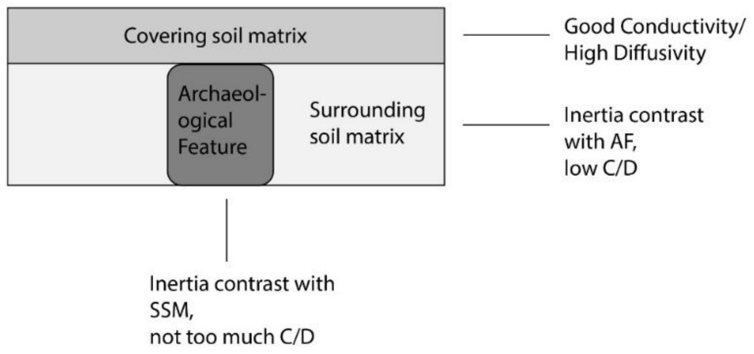
2. Theory: The Mechanics of Thermography
A Systematic Approach
3. Materials and Methods
3.1. Recording Heat
3.2. Analyzing Heat
4. Results
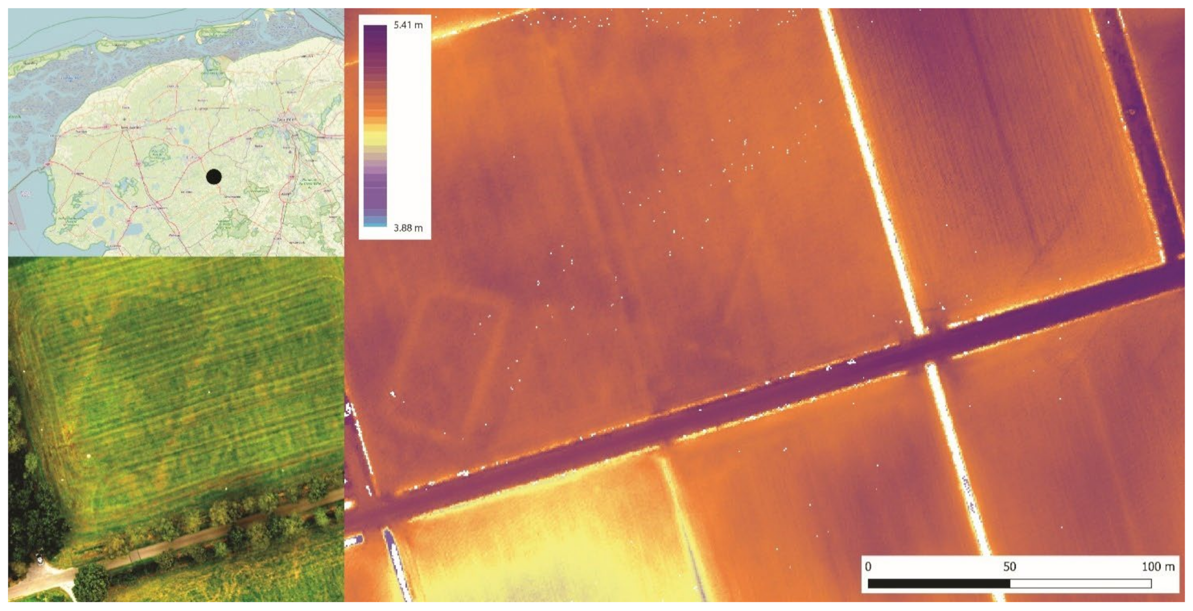
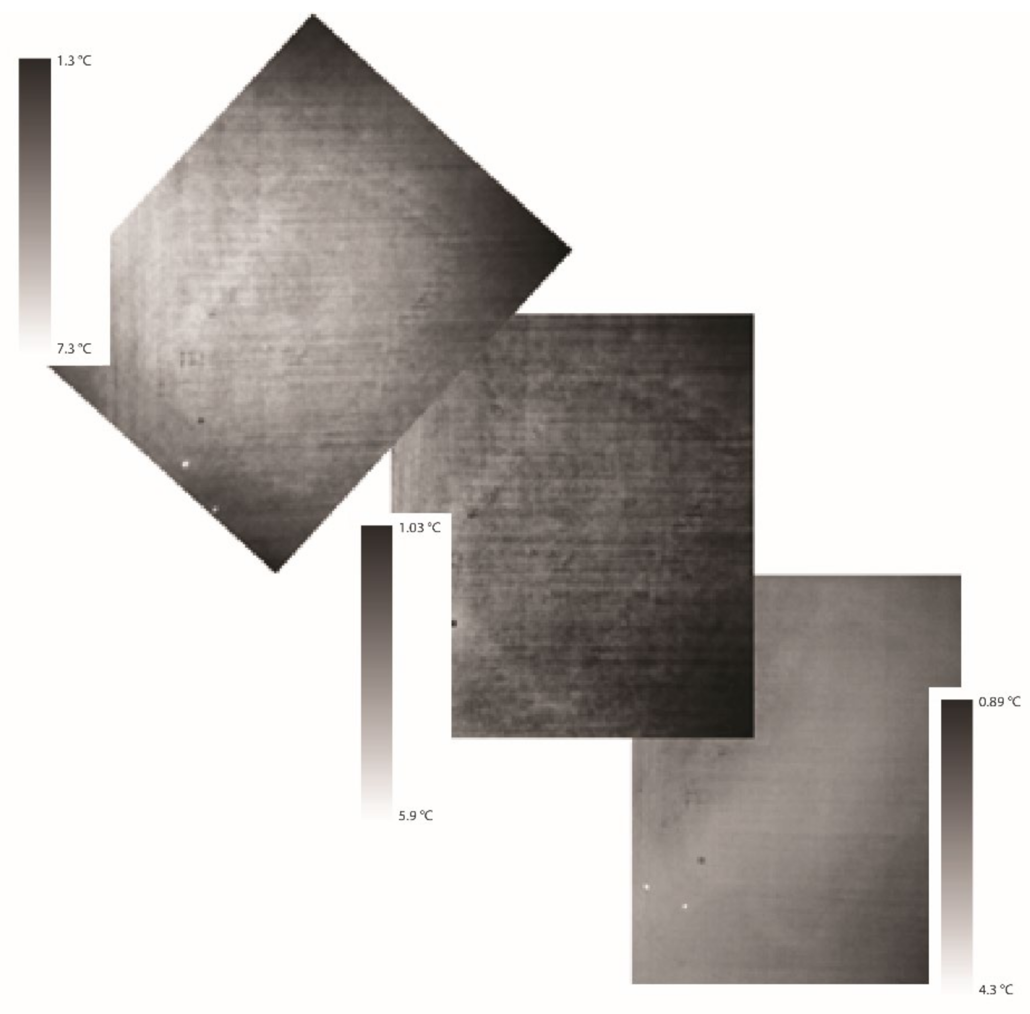
4.1. Siegerswoude
4.1.1. Thermography Capturing Strategy and Conditions
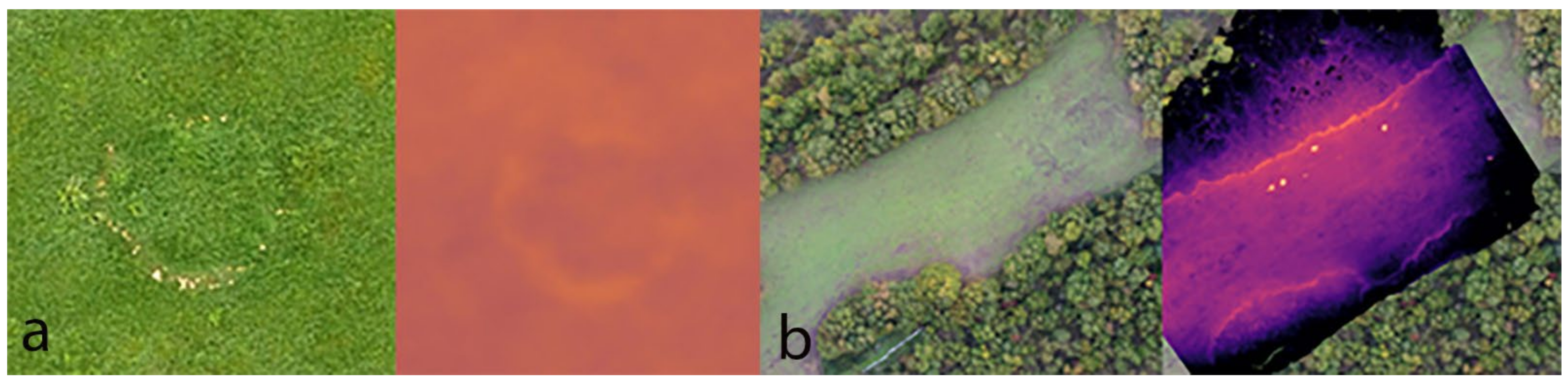
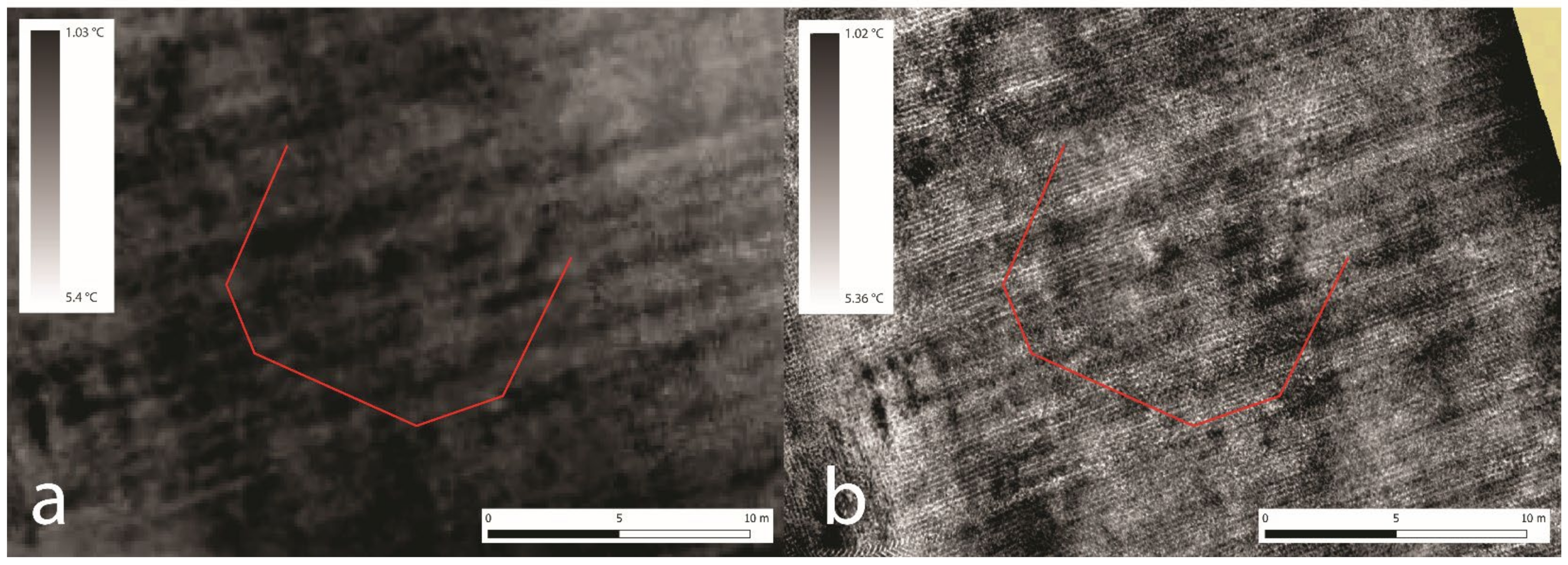
4.1.2. Spectral Marks
4.1.3. Excavations
4.1.4. Interpretations
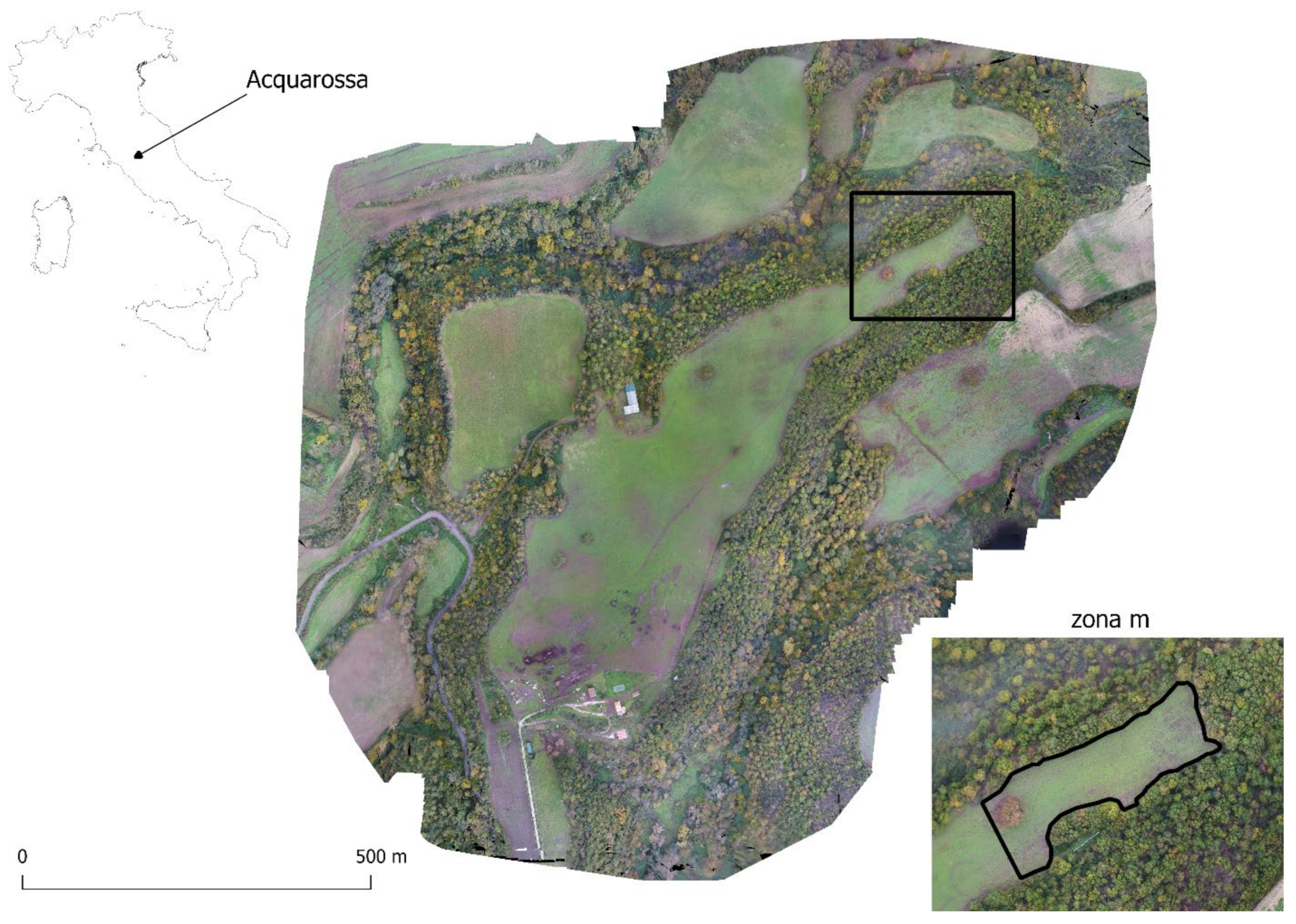
4.2. Acquarossa
4.2.1. Thermography Capturing Strategy and Conditions
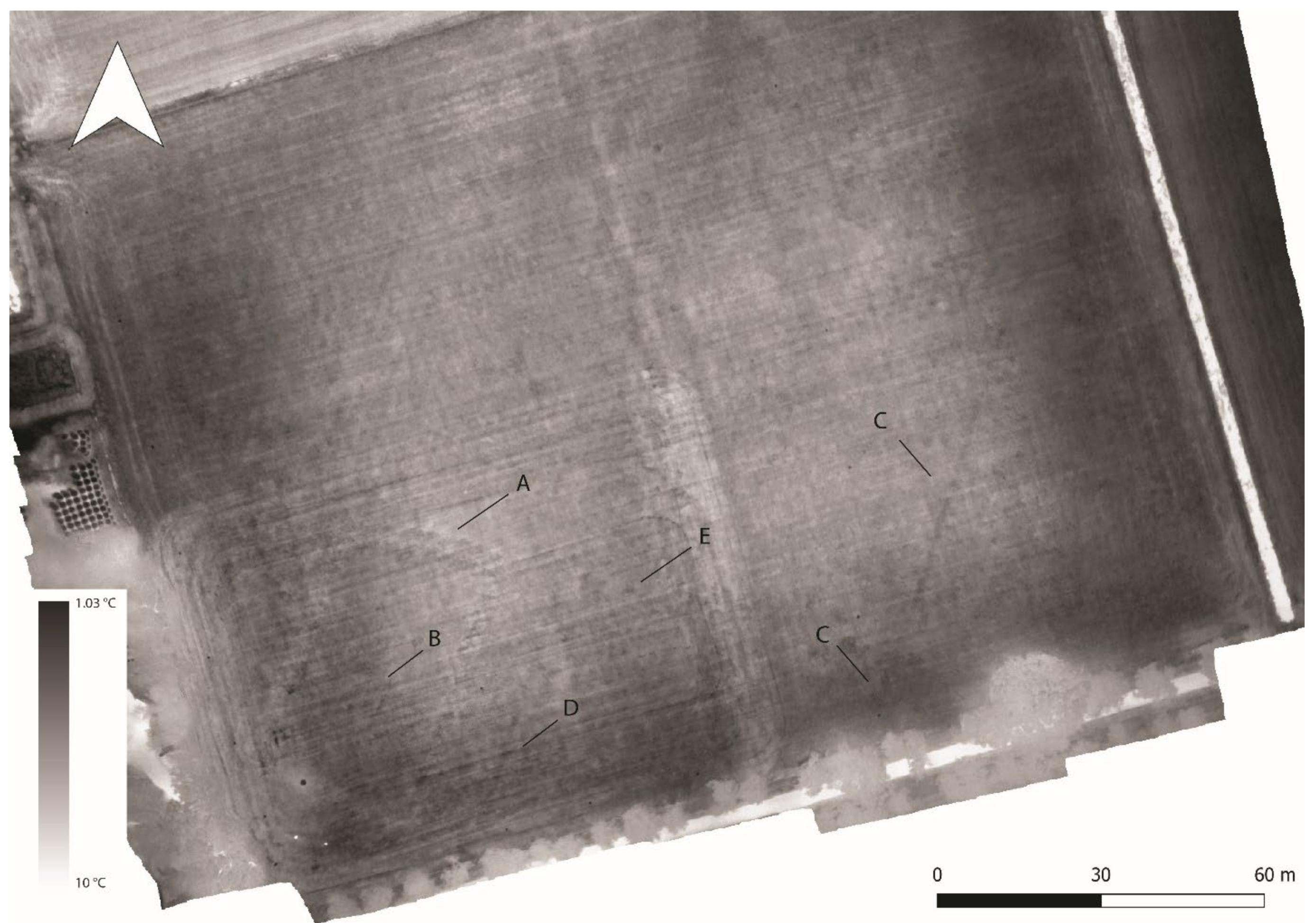
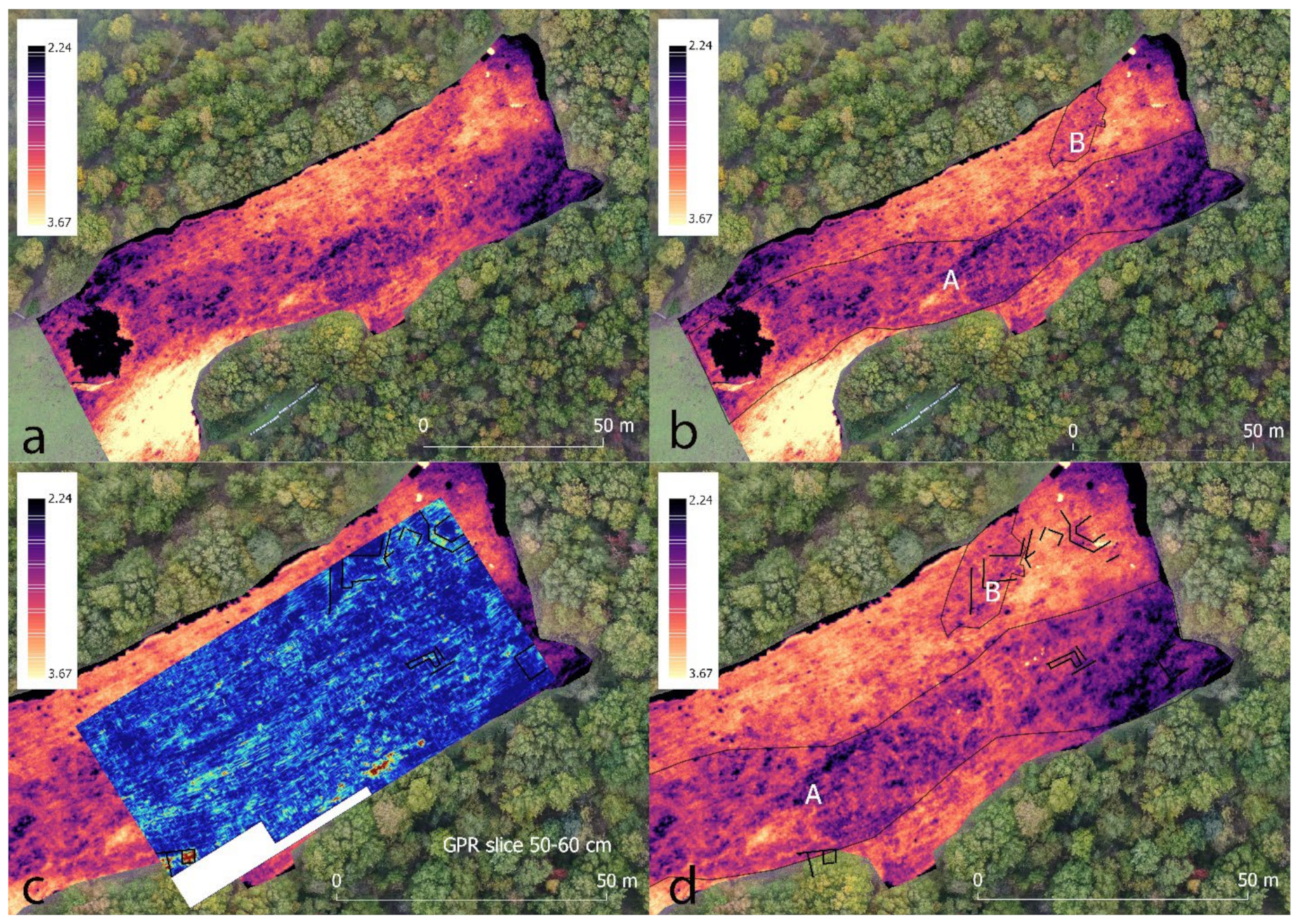
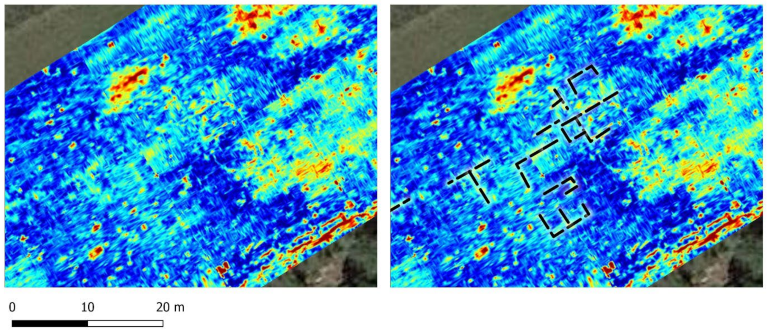
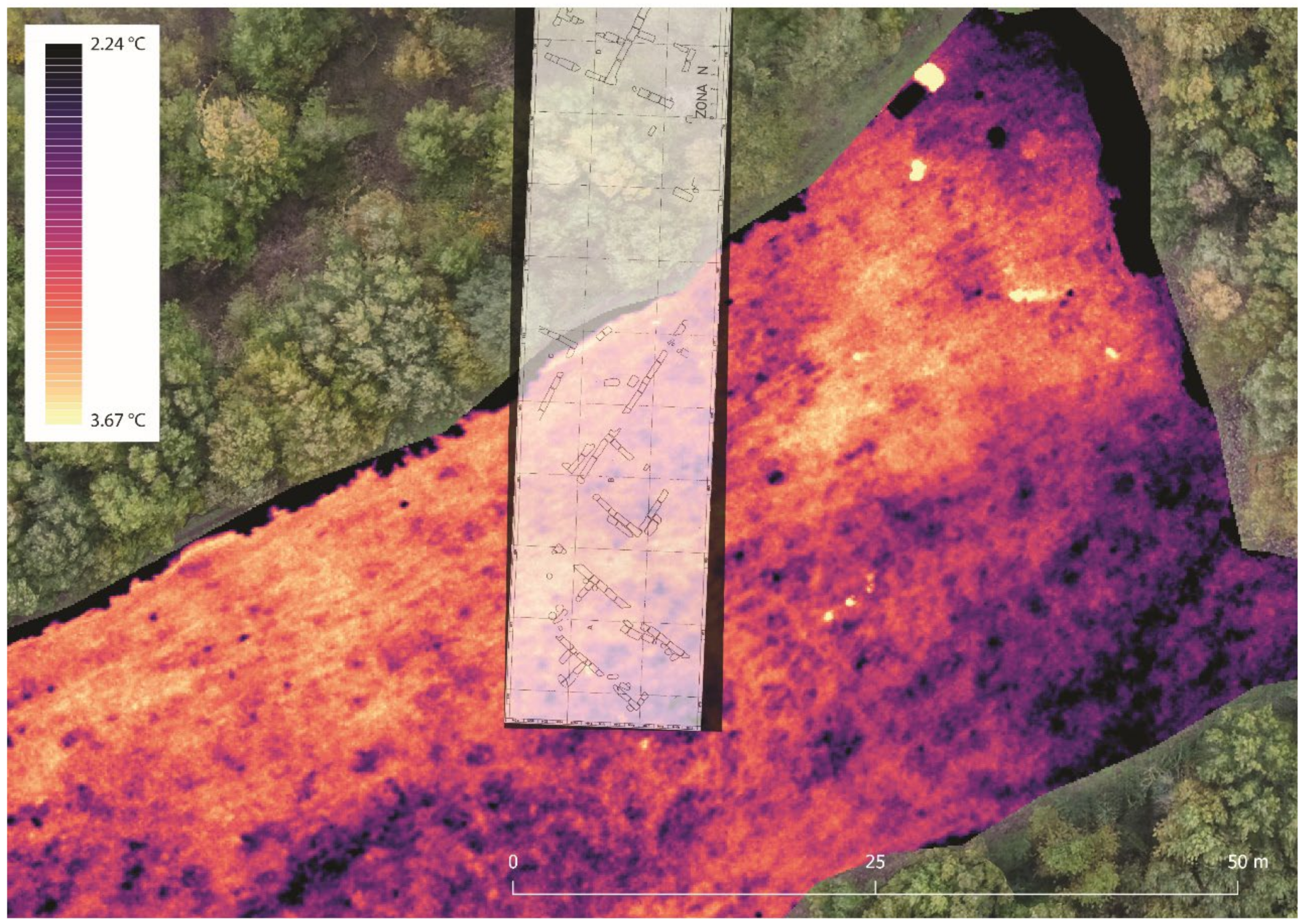
4.2.2. Spectral Marks
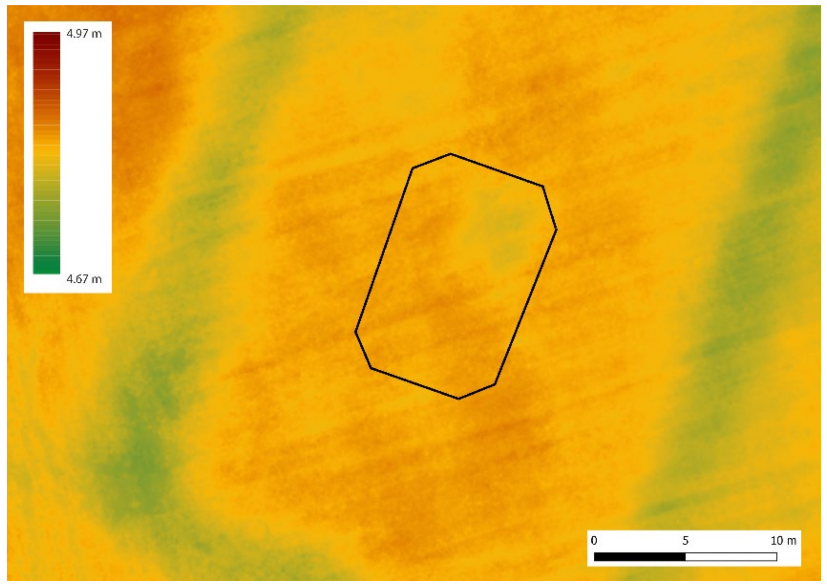
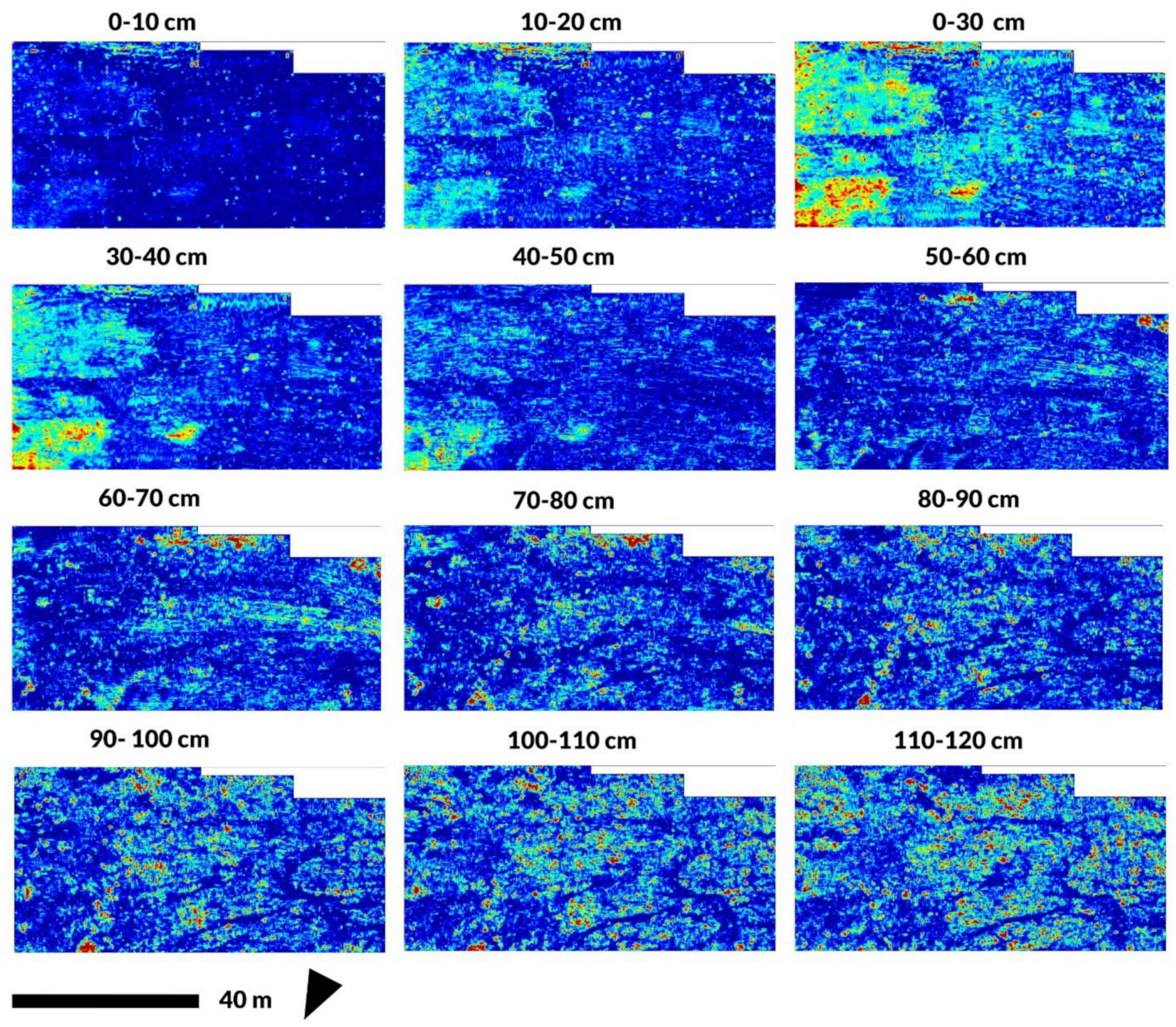
4.2.3. Ground-Penetrating Radar
4.2.4. Interpretations
5. Discussion. The Performance of Drone Thermography in a Comparative View
6. Conclusions
Author Contributions
Funding
Institutional Review Board Statement
Informed Consent Statement
Data Availability Statement
Acknowledgments
Conflicts of Interest
References
- Perisset, M.C.; Tabbagh, A. Interpretation of Thermal Prospection on Bare Soils. Archaeometry 1981, 23, 169–187. [Google Scholar] [CrossRef]
- Scollar, I.; Hesse, A.; Herzog, A.; Tabbagh, A. Archaeological Prospecting and Remote Sensing; Cambridge University Press: Cambridge, UK, 1990. [Google Scholar]
- Giardino, M.; Bryan, S.H. Airborne Remote Sensing and Geospatial Analysis. In Remote Sensing in Archaeology: An Explicitly North American Perspective; Johnson, J.K., Ed.; University of Alabama Press: Tuscaloosa, AL, USA, 2006; pp. 47–77. [Google Scholar]
- Kvamme, K.L. Integrating Multidimensional Geophysical Data. Archaeol. Prospect. 2006, 13, 57–72. [Google Scholar] [CrossRef]
- Verhoeven, G. The reflection of two fields—Electromagnetic radiation and its role in (aerial) imaging. AARGnews 2017, 55, 13–18. [Google Scholar]
- Cool, A.C. Thermography. In The Encyclopedia of Archaeological Sciences; López Varela, L.S., Ed.; Wiley: Hoboken, NJ, USA, 2018; pp. 1–5. [Google Scholar] [CrossRef]
- Poirier, N.; Hautefeuille, F.; Calastrenc, C. Low altitude thermal survey by means of an automated unmanned aerial vehicle for the detection of archaeological buried structures. Archaeol. Prospect. 2013, 20, 303–307. [Google Scholar] [CrossRef] [Green Version]
- Casana, J.; Kantner, J.; Wiewel, A.; Cothren, J. Archaeological Aerial Thermography: A Case Study at the Chaco-Era Blue J Community, New Mexico. J. Archaeol. Sci. 2014, 45, 207–219. [Google Scholar] [CrossRef]
- Casana, J.; Wiewel, A.; Cool, A.C.; Hill, A.C.; Fisher, K.D.; Laugier, E.J. Archaeological Aerial Thermography in Theory and Practice. Adv. Archaeol. Pract. 2017, 5, 310–327. [Google Scholar] [CrossRef] [Green Version]
- Thomas, H. Some like it hot: The impact of next generation FLIR Systems thermal cameras on archaeological thermography. Archaeol. Prospect. 2018, 25, 81–87. [Google Scholar] [CrossRef]
- Agudo, P.U.; Pajas, J.A.; Pérez-Cabello, F.; Redón, J.V.; Lebrón, B.E. The Potential of Drones and Sensors to Enhance Detection of Archaeological Cropmarks: A Comparative Study Between Multi-Spectral and Thermal Imagery. Drones 2018, 2, 29. [Google Scholar] [CrossRef] [Green Version]
- McLeester, M.; Casana, J.; Schurr, M.R.; Hill, A.C.; Wheeler, J.H. Detecting prehistoric landscape features using thermal, multispectral, and historical imagery analysis at Midewin National Tallgrass Prairie, Illinois. J. Archaeol. Sci. Rep. 2018, 21, 450–459. [Google Scholar] [CrossRef]
- Hill, A.C.; Laugier, E.; Casana, J. Archaeological Remote Sensing Using Multi-Temporal, Drone Acquired Thermal and Near Infrared (NIR) Imagery: A Case Study at the Enfield Shaker Village, New Hampshire. Remote Sens. 2020, 12, 690. [Google Scholar] [CrossRef] [Green Version]
- James, K.; Nichol, C.J.; Wade, T.; Cowley, D.; Gibson Poole, S.; Gray, A.; Gillespie, J. Thermal and Multispectral Remote Sensing for the Detection and Analysis of Archaeologically Induced Crop Stress at a UK Site. Drones 2020, 4, 61. [Google Scholar] [CrossRef]
- Salgado Carmona, J.Á.; Quirós, E.; Mayoral, V.; Charro, C. Assessing the potential of multispectral and thermal UAV imagery from archaeological sites: A case study from the Iron Age hillfort of Villasviejas del Tamuja (Cáceres, Spain). J. Archaeol. Sci. Rep. 2020, 31, 102312. [Google Scholar] [CrossRef]
- Cowley, D.; Verhoeven, G.; Traviglia, A. Editorial for Special Issue: “Archaeological Remote Sensing in the 21st Century: (Re)Defining Practice and Theory”. Remote Sens. 2021, 13, 1431. [Google Scholar] [CrossRef]
- Baroň, I.; Beĉkovský, D.; Míĉa, L. Application of infrared thermography for mapping open fractures in deep-seated rockslides and unstable cliffs. Landslides 2014, 11, 15–27. [Google Scholar] [CrossRef]
- De Reu, J.; Plets, G.; Verhoeven, G.; De Smedt, P.; Bats, M.; Cherretté, B.; De Maeyer, W.; Deconynck, J.; Herremans, D.; Laloo, P.; et al. Towards a three-dimensional cost-effective registration of the archaeological heritage. J. Archaeol. Sci. 2013, 40, 1108–1121. [Google Scholar] [CrossRef]
- Sapirstein, P. Accurate measurement with photogrammetry at large sites. J. Archaeol. Sci. 2016, 66, 137–145. [Google Scholar] [CrossRef]
- Sapirstein, P.; Murray, S. Establishing Best Practices for Photogrammetric Recording During Archaeological Fieldwork. J. Field Archaeol. 2017, 42, 337–350. [Google Scholar] [CrossRef]
- Waagen, J. New technology and archaeological practice. Improving the primary archaeological recording process in excavation by means of UAS photogrammetry. J. Archaeol. Sci. 2019, 101, 11–20. [Google Scholar] [CrossRef]
- Walker, S. Low-altitude aerial thermography for the archaeological investigation of arctic landscapes. J. Archaeol. Sci. 2020, 117, 105126. [Google Scholar] [CrossRef]
- Van Doesburg, J.; Van der Heiden, M.; Waagen, J.; Van Os, B.; Van der Meer, W. Op Zoek NAAR Lijnen: Onderzoek naar de Bruikbaarheid van Elektromagnetische Inductie en Optische en een Thermische Infraroodbeelden voor de Archeologie in Siegerswoude (Provincie Friesland); Archeologische Monumentenzorg: Amersfoort, The Netherlands, 2022. [Google Scholar]
- Worst, D. Agrarische Veenontginningen in Oostelijk Opsterland (900–1700 AD): Een Interdisciplinair Onderzoek naar de Natuurlijke Landschapsopbouw, de Nederzettings–En Ontginningsgeschiedenis en Het Agrarische Landgebruik Langs de Boven—En Middenloop van het Koningsdiep. Master’s Thesis, Rijksuniversiteit Groningen, Elsloo, The Netherlands, 2012. [Google Scholar]
- Seyfried, S. Thermal and Multispectral Monitoring of cropmarks by UAV. AARGnews 2020, 61, 52–55. [Google Scholar]
- Lulof, P.S.; Sepers, M.H. The Acquarossa memory project. Reconstructing an Etruscan town. Archeol. Calc. 2017, 28, 233–242. [Google Scholar]
- Lulof, P.S. Recreating Reconstructions: Archaeology, Architecture and 3D Technologies. In Reconstruction, Replication and Re-enactment in the Humanities and Social Sciences; Dupré, S., Harris, A., Kursell, J., Lulof, P.S., Stols-Witlox, M., Eds.; Amsterdam University Press: Amsterdam, The Netherlands, 2021; pp. 253–274. [Google Scholar]
- Östenberg, C.E. Case Etrusche di Acquarossa; Multigrafica: Rome, Italy, 1975. [Google Scholar]
- Wikander, O. Acquarossa VI: The Roof-Tiles, 1—Catalogue and Architectural Context; Paul Astroms Forlag: Stockholm, Sweden, 1986. [Google Scholar]
- Östenberg, C.E. Acquarossa—Ferentium: Campagna di Scavo 1975. Opusc. Romana 1976, 11, 3. [Google Scholar]
- Laloui, L.; Rotta Loria, A.F. Analysis and Design of Energy Geostructures, Theoretical Essentials and Practical Application; Academic Press: Cambridge, MA, USA, 2019. [Google Scholar]
- Conyers, L.B. Ground—Penetrating Radar for Archaeology; AltaMira Press: Walnut Creek, CA, USA, 2004. [Google Scholar]
- Goodman, D. GPR Methods for Archaeology; Springer: Berlin/Heidelberg, Germany, 2013; Available online: https://www.taylorfrancis.com/ (accessed on 5 November 2020).
- Goodman, D.; Piro, S. GPR Remote Sensing in Archaeology; Springer: New York, NY, USA, 2013. [Google Scholar]
- Catapano, I.; Gennarelli, G.; Ludeno, G.; Soldovieri, F. Applying Ground-Penetrating Radar and Microwave Tomography Data Processing in Cultural Heritage: State of the Art and Future Trends. IEEE Signal Process. Mag. 2019, 36, 53–61. [Google Scholar] [CrossRef]
- Seren, S.; Eder-Hinterleitner, A.; Neubauer, W.; Melichar, P. Extended comparison of different GPR systems and antenna configurations at the Roman site of Carnuntum. Near Surf. Geophys. 2007, 5, 389–394. [Google Scholar] [CrossRef]
- García Sánchez, J.; Costa-García, J.M. Remote Sensing and Geophysical Survey in Veladiez. A New Sector of the Roman Town of Segisamo (Sasamón, Burgos). Rev. Xeol. Galega Hercínico Penins. 2021, 43, 41–60. [Google Scholar]
- Sarris, A.; Kalayci, T.; Papadopoulos, N.; Argyriou, N.; Donati, J.; Kakoulaki, G.; Manataki, M.; Papadakis, M.; Nikas, N.; Scotton, P.; et al. Geophysical explorations of the classical coastal settlement of Lechaion, Peloponnese (Greece). Mapp. Past 2020, 1, 43–52. [Google Scholar]
- Holst, G.C. Common Sense Approach to Thermal Imaging; JDC Publishing: Norwalk, CA, USA, 2000. [Google Scholar]


| Variable | Explanation/Example |
|---|---|
| Flight altitude | 10, 30 or 100 m |
| Current temperature | Temperature at time of flight, record from local weather station, °C |
| Day temperature | Maximum daily temperature, record from local weather station, °C |
| Night temperature | Minimum nightly temperature, record from local weather station, °C |
| Long-term heat flux | Significant change in temperature patterns in the preceding days |
| Light conditions | Short-term variability in cloud cover, i.e., clear, overcast, etc. |
| Surface anomalies | Record presence, i.e., of reflective materials, potential effect on thermal recordings, i.e., water, metal objects, etc. |
| Relative humidity | Record from local weather station, % |
| Moisture conditions | Record whether the soil is moist, whether there has been rain |
| Irrigation | Have the fields been watered? |
| Vegetation type/land use | Brushes, wheat, grass, etc. |
| Estimated depth | Of archaeological remains, cm |
| Superficial layer | Composition of topsoil layer |
| Soil matrix | Composition of surrounding soil matrix (of archaeological features) |
| Expected features | What archaeology is expected (i.e., stone walls) |
| Topographic features | Ridges, ditches, protruding bedrock |
| Surface archaeology | Any visible archaeology above ground (structures, surface artefacts, etc.) |
Publisher’s Note: MDPI stays neutral with regard to jurisdictional claims in published maps and institutional affiliations. |
© 2022 by the authors. Licensee MDPI, Basel, Switzerland. This article is an open access article distributed under the terms and conditions of the Creative Commons Attribution (CC BY) license (https://creativecommons.org/licenses/by/4.0/).
Share and Cite
Waagen, J.; Sánchez, J.G.; van der Heiden, M.; Kuiters, A.; Lulof, P. In the Heat of the Night: Comparative Assessment of Drone Thermography at the Archaeological Sites of Acquarossa, Italy, and Siegerswoude, The Netherlands. Drones 2022, 6, 165. https://doi.org/10.3390/drones6070165
Waagen J, Sánchez JG, van der Heiden M, Kuiters A, Lulof P. In the Heat of the Night: Comparative Assessment of Drone Thermography at the Archaeological Sites of Acquarossa, Italy, and Siegerswoude, The Netherlands. Drones. 2022; 6(7):165. https://doi.org/10.3390/drones6070165
Chicago/Turabian StyleWaagen, Jitte, Jesús García Sánchez, Menno van der Heiden, Aaricia Kuiters, and Patricia Lulof. 2022. "In the Heat of the Night: Comparative Assessment of Drone Thermography at the Archaeological Sites of Acquarossa, Italy, and Siegerswoude, The Netherlands" Drones 6, no. 7: 165. https://doi.org/10.3390/drones6070165