Article

Comparison of Machine Learning Algorithms for Wildland-Urban Interface Fuelbreak Planning Integrating ALS and UAV-Borne LiDAR Data and Multispectral Images

by
Francisco Rodríguez-Puerta
1,2,3,*,
Rafael Alonso Ponce
2,3,
Fernando Pérez-Rodríguez
2,
Beatriz Águeda
1,2,3,
Saray Martín-García
2,4,
Raquel Martínez-Rodrigo
2,3 and
Iñigo Lizarralde
2,3
1
EiFAB, Campus Duques de Soria s/n, Universidad de Valladolid, 42004 Soria, Spain
2
Föra Forest Technologies sll, Campus Duques de Soria s/n, 42004 Soria, Spain
3
Sustainable Forest Management Research Institute, University of Valladolid-INIA, Campus Duques de Soria s/n, 42004 Soria, Spain
4
Biodiversity-LaboraTe-IBADER, Departamento de Enxeñaría Agroforestal, Universidade de Santiago de Compostela, 27001 Lugo, Spain
*
Author to whom correspondence should be addressed.
Drones 2020, 4(2), 21; https://doi.org/10.3390/drones4020021
Submission received: 19 May 2020 / Revised: 10 June 2020 / Accepted: 10 June 2020 / Published: 11 June 2020

Abstract

:
Controlling vegetation fuels around human settlements is a crucial strategy for reducing fire severity in forests, buildings and infrastructure, as well as protecting human lives. Each country has its own regulations in this respect, but they all have in common that by reducing fuel load, we in turn reduce the intensity and severity of the fire. The use of Unmanned Aerial Vehicles (UAV)-acquired data combined with other passive and active remote sensing data has the greatest performance to planning Wildland-Urban Interface (WUI) fuelbreak through machine learning algorithms. Nine remote sensing data sources (active and passive) and four supervised classification algorithms (Random Forest, Linear and Radial Support Vector Machine and Artificial Neural Networks) were tested to classify five fuel-area types. We used very high-density Light Detection and Ranging (LiDAR) data acquired by UAV (154 returns·m−2 and ortho-mosaic of 5-cm pixel), multispectral data from the satellites Pleiades-1B and Sentinel-2, and low-density LiDAR data acquired by Airborne Laser Scanning (ALS) (0.5 returns·m−2, ortho-mosaic of 25 cm pixels). Through the Variable Selection Using Random Forest (VSURF) procedure, a pre-selection of final variables was carried out to train the model. The four algorithms were compared, and it was concluded that the differences among them in overall accuracy (OA) on training datasets were negligible. Although the highest accuracy in the training step was obtained in SVML (OA=94.46%) and in testing in ANN (OA=91.91%), Random Forest was considered to be the most reliable algorithm, since it produced more consistent predictions due to the smaller differences between training and testing performance. Using a combination of Sentinel-2 and the two LiDAR data (UAV and ALS), Random Forest obtained an OA of 90.66% in training and of 91.80% in testing datasets. The differences in accuracy between the data sources used are much greater than between algorithms. LiDAR growth metrics calculated using point clouds in different dates and multispectral information from different seasons of the year are the most important variables in the classification. Our results support the essential role of UAVs in fuelbreak planning and management and thus, in the prevention of forest fires.

1. Introduction

Since the 1950s, a global phenomenon of rural-to-urban migration has been taking place, mainly in developed countries, leading to profound changes in land use caused by rural abandonment. Though the extent and effects of these changes in rural landscapes vary significantly among regions, in the Mediterranean basin one of the negative consequences is the increase in frequency and intensity of wildfires due to the encroachment of shrublands and young forests into ancient farmlands and pastures [1]. In many cases, the traditional domus, hortus, ager, saltus and silva system has been transformed into a prevalent wildland-urban interface (WUI) [2] in rural areas. This situation becomes particularly unmanageable when the structure of the human settlements is scattered.
In this scenario, controlling vegetation fuels around human settlements is a critical strategy to reduce fire severity in forests, buildings and infrastructures [1]. These specific areas can be synthetically classified into firebreaks and fuel-breaks. In both cases they are fuel-managed areas dedicated to stopping or reducing fire propagation, respectively. Firebreaks are areas of land (usually linear in shape) where the fuel present is completely removed, while fuelbreaks are usually wider, and covered by vegetation, where the fuel is partially removed [3]. When some forest canopy remains after treatment they are referred to as shaded fuelbreaks [1].
Fuelbreaks at the WUI consist of modifying the fuel load in areas adjacent to buildings and infrastructure in order to reduce the probability of ignition and the severity of a potential wildfire and thus to create safer areas for firefighting [4,5]. According to Ascoli et al. [3], in general, a surface fuel load ranging from 0.2 to 0.4 kg·m
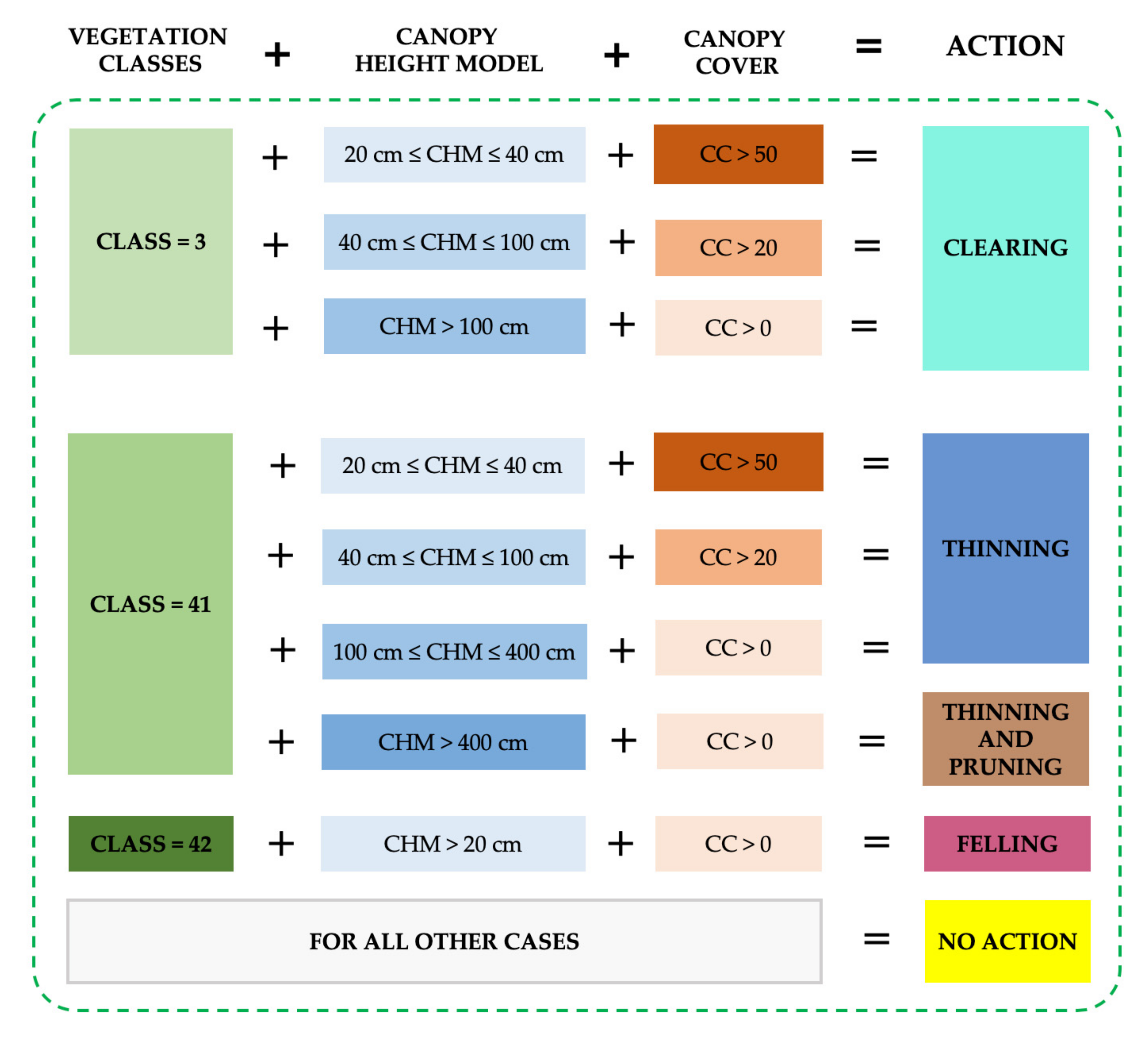
−2 is recommended for fuelbreaks. Regarding canopy cover, a value between 10% and 50% is desirable, while a crown base height of more than 2.5–5 m is recommended (depending on the surface fuels available) to avoid vertical continuity of the fuel. Finally, they recommend a recurrence in the operations ranging from 1 to 6 years. Even so, the rules for establishing the recommended fuel load and the permitted vegetation type depend on the legislation of each country. This legislation is generally in agreement with the forest and ownership structures of the area. In addition, the rules for firebreaks always depend on two factors; firstly, on the type of vegetation, and then on its characteristics, usually evaluated based on the height of the trees and their canopy cover.
In this case, these rules are based on the fact that the typical Galician forest was mainly made up of deciduous species, such as oak (Quercus robur L.), chestnut tree (Castanea sativa Mill.), and maritime pine (Pinus pinaster Ait.), but these formations have been greatly reduced through centuries in favor of pastures, agricultural land and shrublands. During the 20th century a remarkable increment in forested area took place, mainly through reforestations with maritime pine and the foreign species blue gum (Eucalyptus globulus Labill.), which has transformed the Galician forest environment into a pine- and eucalyptus-dominated landscape. In fact, these two species, along with the species of the genus Acacia Mill. have been declared forbidden in the fuelbreaks of the WUIs.
To characterize the forest structure, and especially to perform classifications, it is common to use remote sensing technologies, both optical satellite imagery and airborne Light Detection And Ranging (LiDAR). Optical satellite imagery is considered passive data, while LiDAR is considered an active sensor. The purpose of image fusion is to use different types of sensor data to obtain more information from their union than is possible from separate analyses [6]. In this way, the integration of LiDAR data and multispectral imagery provides the geometric and radiometric attributes, respectively [7]. Different authors [8,9] have preferred to use only active sensors, which provide values related to vegetation metrics, while others [10,11,12,13,14] have privileged the combination of multispectral imagery with LiDAR information to improve classification accuracies in forest environments. In all cases, the use of remote sensing substantially reduces the cost of the estimation process [15].
A drone or Unmanned Aerial Vehicle (UAV) is a lightweight flying device that is not operated by an on-board pilot, and also has a ground control station and communication components. These devices can be either self-controlled or remotely piloted. Based on the types of wing, UAVs might broadly be classified as fixed-wing or rotary-wing type. Finally, they are classified according to the weight of their platform; thus, the most interesting ones for evaluating vegetation are usually the small unmanned aerial systems (UAS) whose weight is less than 10 kg [16].
Although the origin of UAS dates back to the military sector, especially to surveillance, in recent decades their professional use has become widespread in aerial photography and also in remote sensing [17]. Nowadays, it has become a common working tool in many fields such as forestry, precision agriculture and other sectors related to civil engineering, as well as emergency response [18]. On the other hand, the incorporation of cloud-based and generally more user-friendly data processing systems has greatly helped its expansion as a working tool [19].
Algorithms based on Machine Learning techniques such as Random Forests (RF) are now widely used for classification and prediction purposes in remote sensing applications [20]. Nevertheless, the Artificial Neural Networks (ANN) and Linear and Radial Support Vector Machine (SVML, SVMR) algorithms are increasingly being taken into consideration [21,22,23]. All these algorithms have been successfully applied to estimate forest biophysical parameters through multispectral data [24], biomass and soil moisture recovery [25], crop monitoring [26] or land use classification [27,28,29]. However, RF is the most widely used algorithm for earth observation and, in particular, for classification of land use and forestry applications [30]. Among different studies, we can highlight the use of RF to detect insect infestations according to the physiological characteristics of plants [31] or to estimate timber production [32] and forest biomass [33]. Nevertheless, other authors [34] consider that SVM is the best algorithm to solve complex classification problems, such as differentiation of tree species. Recently, due to the great success that deep learning is having, ANN are being used extensively for remote sensing in Earth observation and often achieve the same accuracies as SVML or even RF [28].
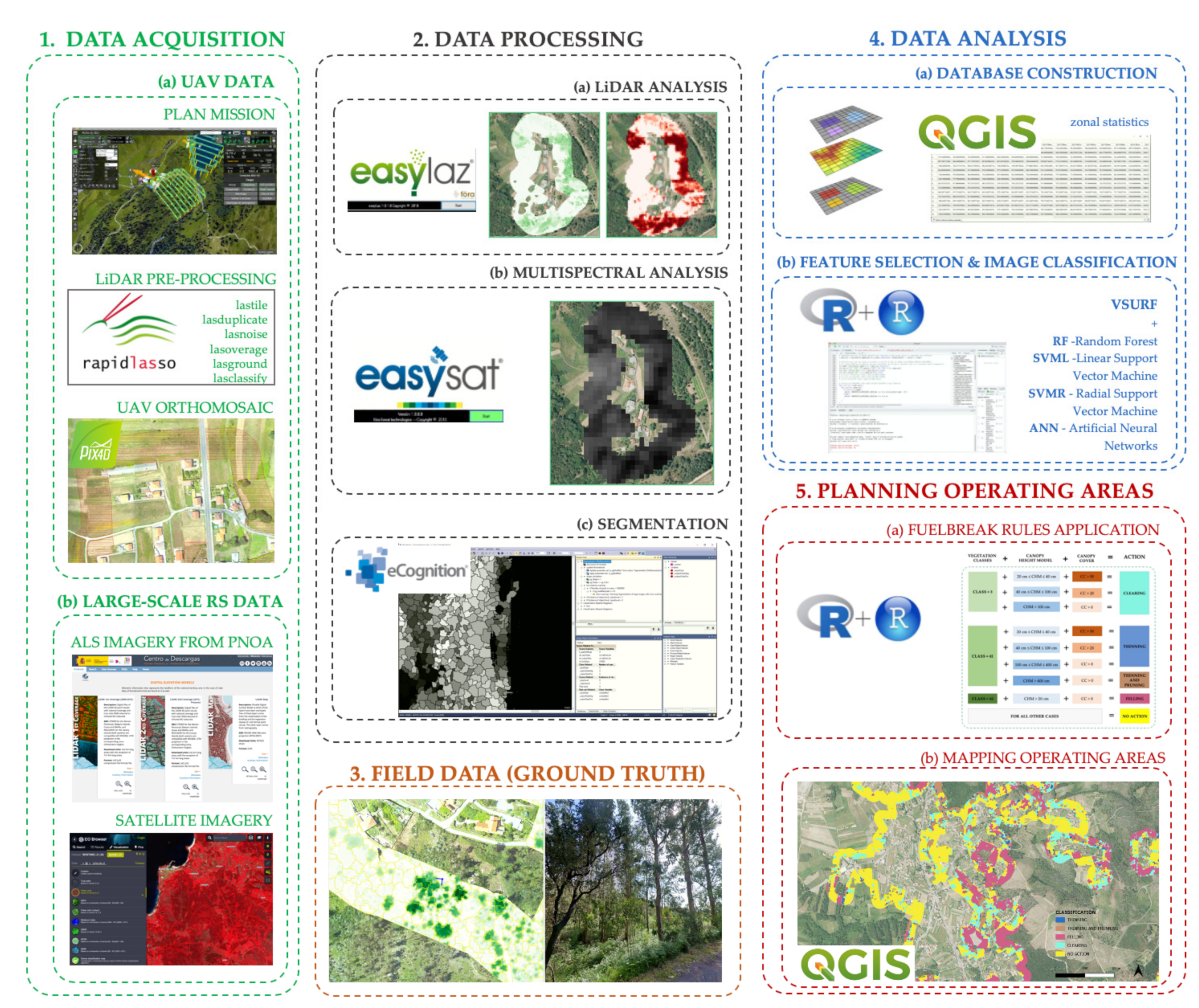
Based on the initial hypothesis that UAVs could be used to identify action areas in fuelbreaks and WUI areas, the general objective of this work is to test the performance of combined passive and active remote sensing data to predict vegetation types through machine learning algorithms. More specifically, we aim at: (i) analyzing the uncertainty of these four classification methods (RF, SVML, SVMR and ANN) in an object-based approach; (ii) comparing the accuracy obtained by different combinations of active and passive remote data sensed (UAV-LiDAR, low density LiDAR and different satellite images) and their interaction with the four ML algorithms; and finally (iii) mapping the wildland-urban interface fuelbreak planning rules.

2. Materials and Methods

2.1. Study Area

The study area is located in Porto do Son (Galicia, Northwest Spain). The municipality of Porto do Son encompasses a collection of coastal towns and scattered inland villages. The most represented tree species in the area are chestnut (Castanea sativa), oak (Quercus robur), pine (Pinus pinaster) and eucalyptus (Eucalyptus globulus). The climate of the area is characterized by high rainfall, low temperature variation, mild temperatures and some water deficit in summer. The main characteristics of the atmospheric environment are linked to the influence of the sea. The area of interest of this location corresponded to 3.7 km2 (Figure 1).

2.2. Data Acquisition

2.2.1. UAV Imagery

Data from the UAV was obtained in July 2019. The integrated LiDAR system comprises a DJI M600 Pro UAV, a Phoenix LiDAR Systems Scout 16 with a Velodyne VLP-16 LiDAR sensor, an A6K RGB camera (based on Sony A600) and an inertial measurement unit (IMU-14). It is a high-precision system (Root Mean Square Error (RMSE) = 30 mm) with a scanning rate of 600 k dual return points/s with a 360-degree field of view at a recommended scanning height of 20–60 m. To generate Post-Processing Kinematic paths (PPK) the system uses a dual-frequency L1/L2 Global Navigation Satellite System (GNNS) receiver. The study was conducted with a flight height of 55 m above the ground at a speed of 4 m/s and at an approximate horizontal distance between adjacent flight lines of 15 m, producing a very high density LiDAR point cloud (154 returns·m−2) with redundant coverage in the 90% overlap area.
Aeromedia UAV Inc. combined IMU and GNSS data through LiDARMill software (Phoenix LiDAR Systems) to apply differential corrections to generate a smooth and highly accurate trajectory for the computation of planimetric coordinates and ellipsoid height values. The LasTools (rapidlasso software) environment was used to pre-process the raw data, which involved five tasks: (i) a total of 586 unbuffered tiles (200 × 200 m) was generated using lastile procedure; (ii) duplicate points were eliminated and noise was reduced using lasduplicate and lasnoise procedures respectively; (iii) the overlap was classified by the procedure lasoverage; (iv) ground points were classified using a triangulated irregular network (TIN) algorithm implemented in lasground_new; (v) and finally the point cloud was classified into vegetation and buildings through the lasclassify procedure [35].
Aeromedia UAV Inc. generated the RGB-orthomosaic (UAV-ORTHO) using the Pix4D software [36]. The overall workflow of Pix4D consists of the following stages: initial photo matching, point cloud densification and ortho mosaic generation. In the case of forest and dense vegetation it is common to modify some parameters both in flight (increase the overlap between images to at least 85% front overlap and at least 70% side overlap) and in process to ensure that the desired quality, accuracy and format of the final production is obtained. The result was a TIFF image with spatial resolution of 4.14 cm and a high level of geometric accuracy (RMSEX,Y = 2.5 cm and RMSEZ = 2.4 cm).

2.2.2. Large-Scale Remote Sensing Data

Two open access ALS point cloud coverages from the National Program of Aerial Orthophotography (PNOA) of the Spanish Government were used (http://centrodedescargas.cnig.es/). The first coverage (ALS1) was collected between February and April 2011, while the second coverage (ALS2) campaign acquired information between July and September 2015. In both coverages, the nominal laser pulse density was 0.5 points·m−2 and the vertical and horizontal accuracy was 0.20 and 0.30 m, respectively. The LiDAR sensor used in each of the datasets was the RIEGL LMS-Q680i and the LEICA ALS60, respectively. In both cases it was mounted on an airplane operated by an on-board pilot.
The digital orthophoto (ORTHO) supplied by the PNOA was also used in this study. In Spain, the PNOA provides annual country-wide coverage with a spatial resolution of at least 0.5 m. An 8-bit RGB orthophoto image, acquired in June 2017, with a spatial resolution of 0.25 m was used.
Two public data sources based on multispectral satellite imagery from the European Space Agency (ESA) Copernicus program were used: (i) Sentinel-2 (S2) satellite images (only the 10 and 20 m resolution bands were considered), and (ii) a Pleiades-1B (P1B) image from the VHR_IMAGE_2015 coverage. We used images from Sentinel-2 captured in February, May, August, and November of the years 2017, 2018 and 2019. These orthorectified and atmospherically corrected images were downloaded from the Copernicus Open Access Hub (https://scihub.copernicus.eu/). Suitable dates were selected to obtain cloud-free and reflection-enhanced images of deciduous trees using easySat® (föra forest technologies) [29]. Pleiades-1B image was captured in July 2015. Copernicus delivers this coverage with an approximate geometric correction. For precise geometric correction, a minimum of nine control points per scene and the DTM with 5 m mesh pitch from the National Plan of Aerial Orthophotography needs to be provided. The maximum allowed error has been 1 m. Table 1 provides detailed information on the spectral and spatial characteristics of each of the bands used.

2.3. Data Processing

2.3.1. LiDAR Analysis

The ALS from PNOA can be downloaded already pre-processed, cleaned and classified. The LiDAR data processing, both from UAV and ALS, consisted also of several steps and was executed with easyLaz® (föra forest technologies), a proprietary tool based on the FUSION/ LDV software [37]. First, Digital Elevation Models were created. The Digital Terrain Model (DTM), using the GridSurfaceCreate procedure, and the Canopy Height Model (CHM), using the CanopyModel procedure, were generated at 0.5 m and 1 m resolution for UAV and at 1 m for ALS, and their respective slope rasters were also obtained. A series of descriptive statistics for a LiDAR data set were calculated by the GridMetrics procedure (Canopy Relief Ratio (CRR), height percentiles (HP) values and Canopy Cover (CC)), all of them with a resolution of 1 m and 5 m for UAV and 5 m for ALS. Finally, and only for data from UAVs, point density metrics were calculated using elevation-based slices in every 1-m height layer through the DensityMetrics procedure. Densities were reported as the proportion of the returns within the layer. Table 2 shows the description of all the raster layers obtained after the LiDAR processing, as well as their spatial resolution.
When two LiDAR datasets were available, height growth metrics were calculated. In the case of the ALS data, since there are two point-clouds coverages, the height growth between the second coverage (ALS2) and the first coverage (ALS1) was calculated, i.e., between 2015 and 2011. Finally, only when UAV and ALS data were combined, then height growth between 2019 (UAV) and 2015 (ALS2) was calculated. A description of the computed variables is shown in Table 3.

2.3.2. Multispectral Analysis

In both image sources (Sentinel-2 and Pleiades-1B), four vegetation indexes were calculated based on imagery data: Enhanced Vegetation Index (EVI), Soil Adjusted Vegetation Index (SAVI), Green Normalized Difference Vegetation Index (GNDVI) and Normalized Difference Vegetation Index (NDVI) [29,38]. Table 4 shows the description of all the raster layers obtained.

2.3.3. Object-Based Image Analysis

Image segmentation is the key to an object-based classification approach. In this way, homogeneous image-objects representing the elements to be classified (e.g., roads, buildings, different types of vegetation) are created by grouping adjacent pixels with homogeneous characteristics [39,40]. An Object-Based Image Analysis was performed through the eCognition (Trimble Geospatial Imaging) software package. This software, like OrfeoToolBox [41] is usually used in remote sensing applications to carry out the segmentation [42]. This object identification is defined accordingly to the specific parameterization of certain attributes such as shape, spectral criterion of homogeneity, scale, and their compactness ratio. Fractal Net Evolution Approach (FNEA) is a multi-resolution segmentation algorithm widely used in object-oriented image analysis. It was first introduced by Baatz and Schäpe [43]. It is based on bottom-up region fusion, i.e., starting with each image pixel as a separate object to merge pixels into large objects at each step, based on relative homogeneity criteria. This homogeneity criterion is a combination of spectral and shape criteria, which are customizable. Higher values of the scale parameter produce larger image objects, and vice versa. However, the homogeneity criterion measures how homogeneous or heterogeneous an image object is within itself. To do this, a combination of the objects’ color and shape properties is used [44]. Finally, eCognition uses a modular programming language (Cognition Network Language) that defines not only the import routines but also the analysis phases of the different objects. In this work three scale parameters (5, 10 and 15) were tested with the aim of finding an optimum parameterization to accurately define objects, and with enough size to compute the spectral information from Sentinel-2 (10 × 10 m) inside each object.

2.4. Field Data

The ground truth was taken at the segment level. Five ground truth classes were defined, as follows: Class 1: No Vegetation; Class 2: Crops; Class 3: Bush and Grass; Class 41: Permitted trees (oak, chestnut tree), and Class 42: Forbidden trees (eucalypt, maritime pine and acacias). During the field work we identified 434 segments (Table 5) distributed through all classes. Once the ground truth was collected, each segment got assigned its vegetation class. Subsequently, zonal statistics were computed for all the variables processed (Table 1, Table 2, Table 3 and Table 4) for the segments of both the ground truth and the entire population.

2.5. Data Analysis

To reduce processing time in model training, feature selection was conducted using the Variable Selection Using Random Forest (VSURF) [45]. VSURF is a consistent three step wrapper-based algorithm which uses RF as the base classifier [46] operating as follows [45]: (i) the thresholding step is focused on removing irrelevant variables from the dataset, (ii) the interpretation step is dedicated to selecting all variables related to the response for interpretation purposes, and (iii) the prediction step improves the selection by removing redundancy in the set of variables selected. The selection of variables is based on the Mean Decrease in Gini (MDG). It is a measure of how important a variable is for estimating the value of the target variable across all the trees that make the Random Forest up. A higher Mean Decrease in Gini indicates higher variable importance. The greater the importance of a variable, the larger the MDG and the higher the position in the plot, and vice versa.
Following Raczko and Zagajewski [47] we compared four nonparametric classification algorithms (ANN, SVML, SVMR, and RF). The Support vector machine (SVM) classifier, developed by Vapnik [48], looks to find the optimal hyperplane in a n-dimensional classification space with the largest margin between classes. SVM was computed using linear and kernel variants. Cost and gamma SVM parameters were established in 1 and the inverse of the number of predictors, respectively. The Random Forest (RF) classifier, developed by Breiman [49], consists of an ensemble of individual decision trees. The maximum number of variables to try in each individual tree was the squared root of the variables selected by VSURF. Maximum number of trees was established in 500. Finally, an ANN classifier can be explained as a parallel computing system consisting of a very large number of simple processors with interconnections. The learning rate was set to 0.3, with a maximum of 105 iterations. To allow the four algorithms compete, the nnet, svmLinear, svmRadial and rf methods were executed using caret package in R software [50].
The ground truth dataset was randomly split in two samples, one for training (70%) and one for testing (30%). The latter was excluded from any training and reserved for testing the performance of the generalization of the model, as this procedure is a key point in supervised classifications aiming at management goals. Next, we executed random k-fold Cross-validation (CV) on the training data set randomly partitioned into folds, which is probably the most popular approach to estimate the error rate, or accuracy, of machine learning-based classifications [51]. A Repeated k-fold CV was performed using 10 folds with three replicas to control overfitting. A 10-fold CV involves dividing the training data set randomly into 10 parts and then using nine parts in training and one part in validation. When using three repeats of 10-fold CV, we will get the average of the error from performing the same analysis three times. This analysis was carried out through the function trainControl (method = “repeatedcv”, number = 10, repeats = 3) of the caret package in R software [50]. Finally, for each classifier, a confusion matrix was computed for predictions of both training and testing datasets.

2.6. Mapping Application of Wildland–Urban Interface Fuelbreak Planning Rules

Once the data had been acquired, processed, the ground truth obtained, the databases created and the prediction of the vegetation class of each segment computed, the wildland-urban interface fuelbreak planning rules were applied (Figure 2). These rules usually include two steps. Firstly, we need to classify the vegetation in every segment following the prediction of the top-performance model. Secondly, we need to calculate the metric for every segment (CHM and CC), which is computed with up-to-date LiDAR information (in our case from UAV-LiDAR).
A general overview of the entire materials and methods used is shown in Figure 3.

3. Results and Discussion

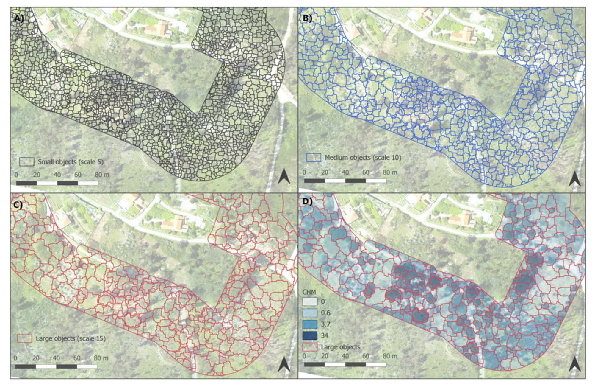
Figure 4 shows the segmentation output. The best result was obtained with a scale parameter of 15. Those segments are large enough to integrate the information from Sentinel-2 indexes (10 × 10 m). A smaller segment size implies too many segments without spectral information because few Sentinel-2 pixel centroids fall inside them.
Depending on the data used, VSURF selects different sets of variables. Table 6 shows the variables selected by VSURF for the different combinations of datasets. In all cases, the variables are sorted by relative importance; the first variable in each column represents the most influential variable in the classification. When two LiDAR point clouds are used, the growth between both point clouds is a crucial variable. In the case where the dataset includes images of Pleiades, these are usually relevant. No fourth-quarter images were selected. Normally, Sentinel images that were selected were from the first quarter and mainly from the NIR or blue band. UAV-LiDAR data are always very significant.
When focusing on results by data source (Table 7), we observe that six of them reach OA >90% for the training dataset at least with one of the algorithms under discussion. Differently, only two of them (ALS + S2 and UAV + ALS + S2) exceeded that figure when generalized to the testing datasets. We hypothesize that, on the one hand, as ALS includes two LiDAR coverages, allowed to estimate the LiDAR-based vegetation growth, which in turn proved to be a relevant variable in the classification procedure. On the other hand, the time series of three complete years (characterized by mean February, May, August and November images) derived from S2 data can satisfactorily characterize the phenology of the different plant species in the area. For those reasons, we consider that the combination ALS + S2 (with or without UAV) is essential to perform optimum classifications in this context. If UAV data are included, results are roughly similar. Nevertheless, we suggest that the use of UAV data should be mandatory to achieve optimum prediction of the actions to be used in the fuelbreak planning. First, UAV data combined with two open access datasets (ALS + S2) reached OA above 90% for all algorithms. Secondly, UAV makes available accurate and updated metrics of the vegetation, which are essential for a correct application of the rules for fuelbreak planning, as they are based not only on the type of vegetation but also on its height.
Regarding the algorithms (Table 7), in 19 combinations of algorithm-data source the OA values surpassed 90% (seven with SVML and SVMR, four with ANN and two with RF). Conversely, only RF accomplished OA values above 90% with more than one data source (i.e., ALS + S2 and UAV + ALS + S2) in the testing phase. In addition, RF was the unique algorithm with OA above 90% with a data source including UAV testing dataset. Furthermore, SVML, SVMR and ANN exhibited larger differences between training and testing OAs, which clearly suggests they tend to overfit. Therefore, we suggest that the best combination analyzed is that combining the dataset UAV + ALS + S2 with the RF algorithm. Consequently, the performance of UAV to identify action areas in fuelbreaks and WUI areas has the greatest accuracy combined with passive and active remote sensing data to predict vegetation types through machine learning algorithms.
Machine Learning-based techniques are suitable tools to optimize classification in land use for fuelbreak planning. Because the differences between the algorithms used are almost negligible (in almost all cases we have an accuracy close to 0.9), it is essential in land use classifications to make all available algorithms compete and also include different databases. In this work, we have found how RF has been the algorithm that offered the most robust results in land use classification purposes in fuelbreak planning due to the small deviation between accuracy values and, more interestingly, more similar values of OA between training and testing datasets. This is particularly relevant when the goal of a supervised classification is to provide managers with operational tools to be applied on large territories far beyond ground truth sample. Over 90% of land use classes (1, 2, 3, 41 and 42) classified from remote sensing data are correct, despite the relatively small size of the ground truth sample. Nevertheless, it is expected that the generalization to a distinct area, even with comparable vegetation attributes, would need an ancillary ground truth sample to retrain the model.
The detailed results of each of the classes separately for all combinations (dataset × algorithm) are shown in Table 8 (training) and Table 9 (testing). When only LiDAR information and orthophotos were used, errors were higher (nearly 20%). When multispectral images were included, errors decreased by 50%, and never exceeded 25%. Class 3 (Bush and Grass) was the one that obtained the less accurate classification results, with errors between 8.3% (SVMR - UAV + SENTINEL) and 36.9% (ANN-UAV). Forbidden tree species (Class = 42) are always classified very precisely, normally obtaining an error below 10%. The Classes (=3; =41 and =42) requiring silvicultural treatments (clearing, thinning, pruning, or felling) tend to be confused with each other when they give false positives. In practice this is not a critical error, since it indicates that a silvicultural treatment must be applied. In any case, the results of both confusion matrices show that it would be advisable to increase the ground truth in the classes with larger errors.
The reliability of Machine Learning for land use classification, in particular for vegetation analysis, has been evaluated in many studies developed in different environments, some of them also based on UAVs combined with other remote sensing data. For example, ref. [22] found that the best ML algorithm to classify forest development stages are RF and ANN, and ref. [23] obtained better results with RF and SVM when classifying mountain forests and shrubland land cover classes. Together with UAV and hyperspectral data [52] used RF to map species in a tropical environment and [53] successfully identified tree species in a mixed coniferous-deciduous forest in the USA. Also, applying Random Forest on UAV images [54] were able to identify seedling stands. The accuracy levels obtained in the present study are consistent with the ones reached in all these previous studies. All this research demonstrates the potential and the efficiency of artificial intelligence to deal with this type of analysis.
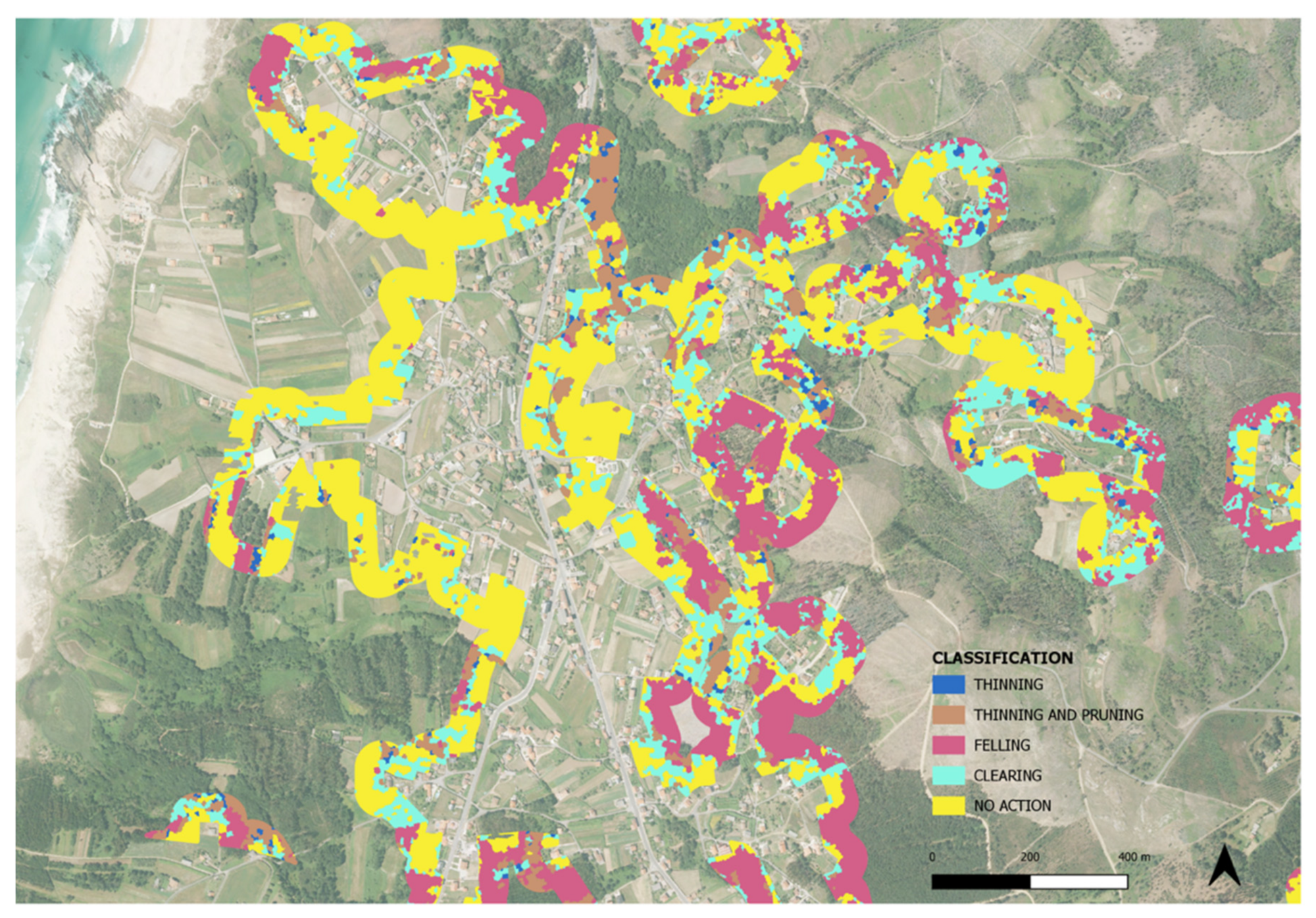
Moreover, the practical implications of using classification techniques for land-use planning at large scale and, particularly for the costly and time-consuming processes usually involved in fuel management, stand out when examining Figure 5. Nearly half of the area of interest studied here is classified as “no action” area, which has the clearest economic consequences. In addition, these data make possible to adequately gauge the required human and machinery resources to carry out the most suitable fuelbreak amount in a given area. Furthermore, since the predicted classification is spatially explicit, it permits not only to plan how many of the attainable resources to deploy before any field exploration, but also where to do it. This would make it feasible to implement optimization procedures [55]. In this regard, the use of high- and very high-resolution DTMs and DSMs derived from the UAV-LiDAR data makes it possible to identify areas with steep slopes and stone fences or other obstacles for machinery, which is crucial for an optimal solution on distribution of resources.
The use of Artificial Intelligence through ML algorithms to classify different land uses is a robust and widely used technique today. It is necessary to make compete algorithms although the differences between precision errors may not seem significant. These differences can become considerable when working on a large scale and without using multispectral imagery. Moreover, differences may not be negligible when classifying larger areas with more types of objects. Thus, the performance of different algorithms and data sources should be tested in every land classification analysis, as their behavior may largely change depending on spectral characteristics, size and variety of the object types included in the study area.

4. Conclusions

In this study, we have shown that UAVs are suitable tools to provide precise and operational data to identify action areas in fuelbreaks of WUI zones. They have the greatest accuracy combined with other passive and active remote sensors to predict vegetation types through machine learning algorithms. No clear differences in the performance of the different ML algorithms have been found. However, we consider RF to be the most robust, providing similar results between training and testing datasets. The rest of the algorithms tend to slightly overfit.
On the contrary, clear differences in prediction ability have been found among different data sources. The use of more than one LiDAR point clouds to calculate vegetation growth provides particularly useful information. The combination of UAV data with large-scale remote sensing data and RF algorithms has an accuracy greater than 0.9 both in training and generalization phases, which makes it an appropriate asset for optimizing vegetation classification for fuelbreak planning. Moreover, the use of UAV should be mandatory whenever other updated LiDAR data are not attainable, as height and cover metrics of vegetation are ineludible to apply actions rules in fuelbreak management planning. Accurate prediction of vegetation type makes possible to adequately gauge the required human and machinery resources to carry out the most suitable fuelbreak amount in a given area, reducing management costs and optimizing field work.
Our results support the essential role of UAVs in fuelbreak planning and management and thus, in the prevention of forest fires and the reduction of damages in human infrastructures and natural environments.

Author Contributions

Conceptualization, F.R.-P., I.L. and R.A.P.; methodology, F.R.-P., R.A.P. and B.Á.; formal analysis and testing, S.M.-G. and R.M.-R.; software, F.P.-R.; writing—original draft preparation, F.R.-P.; writing—review and editing, all authors; project administration, I.L. and R.A.P.; funding acquisition, I.L. and F.R.-P. All authors have read and agreed to the published version of the manuscript.

Funding

This research was funded by the Department of Economy, Industry and Competitiveness, Spanish Government (DI-16-08446, Saray Martín-García; DI-17-09626, Raquel Martínez-Rodrigo; PTQ-16-08411, Beatriz Águeda; PTQ-16-08633, Fernando Pérez-Rodríguez) and by the European Commission through the project ‘MySustainableForest’ (H2020-EO-2017; 776045)

Acknowledgments

LiDAR data was provided by AEROMEDIA UAV and CNIG-PNOA. Satellite imagery was provided by the Plan Nacional de Teledetección (Pleaides images) and the European Space Agency (Sentinel images). The editor and four anonymous reviewers suggested useful comments to improve previous versions of this manuscript.

Conflicts of Interest

The authors declare no conflict of interest.

References

  1. Rey Benayas, J. Abandonment of agricultural land: An overview of drivers and consequences. Cab Rev. Perspect. Agric. Vet. Sci. Nutr. Nat. Resour. 2007, 2. [Google Scholar] [CrossRef] [Green Version]
  2. Langer, E.R.; Pearce, H.G.; Wegner, S. The urban side of the wildland-urban interface: A new fire audience identified following an extreme wildfire event in Aotearoa/New Zealand. In Advances in Forest Fire Research 2018; Imprensa da Universidade de Coimbra: Coimbra, Portugal, 2018; pp. 859–869. ISBN 978-989-26-1650-6. [Google Scholar] [CrossRef] [Green Version]
  3. Ascoli, D.; Russo, L.; Giannino, F.; Siettos, C.; Moreira, F. Firebreak and Fuelbreak. In Encyclopedia of Wildfires and Wildland-Urban Interface (WUI) Fires; Manzello, S.L., Ed.; Springer International Publishing: Cham, Switzerland, 2018; pp. 1–9. ISBN 978-3-319-51727-8. [Google Scholar]
  4. Rigolot, E.; Castelli, L.; Cohen, M.; Costa, M.; Duché, Y. Recommendations for fuel-break design and fuel management at the Wildland Urban Interface: An empirical approach in South Eastern France. In T. Institute of Mediterranean Forest Ecosystems and Forest Products; Warm International Workshop: Athens, Greece, 2004; pp. 131–142. [Google Scholar]
  5. Radeloff, V.C.; Hammer, R.B.; Stewart, S.I.; Fried, J.S.; Holcomb, S.S.; McKeefry, J.F. The Wildland–Urban Interface in the United States. Ecol. Appl. 2005, 15, 799–805. [Google Scholar] [CrossRef] [Green Version]
  6. Wolter, P.T.; Townsend, P.A. Multi-sensor data fusion for estimating forest species composition and abundance in northern Minnesota. Remote Sens. Environ. 2011, 115, 671–691. [Google Scholar] [CrossRef]
  7. Parmehr, E.G.; Amati, M.; Fraser, C.S. Mapping urban tree canopy cover using fused airborne lidar and satellite imagery data. Isprs Ann. Photogramm. Remote Sens. Spat. Inf. Sci. 2016, III–7, 181–186. [Google Scholar] [CrossRef]
  8. González-Olabarria, J.-R.; Rodríguez, F.; Fernández-Landa, A.; Mola-Yudego, B. Mapping fire risk in the Model Forest of Urbión (Spain) based on airborne LiDAR measurements. Ecol. Manag. 2012, 282, 149–156. [Google Scholar] [CrossRef]
  9. González-Ferreiro, E.; Arellano-Pérez, S.; Castedo-Dorado, F.; Hevia, A.; Vega, J.A.; Vega-Nieva, D.; Álvarez-González, J.G.; Ruiz-González, A.D. Modelling the vertical distribution of canopy fuel load using national forest inventory and low-density airbone laser scanning data. PLoS ONE 2017, 12, e0176114. [Google Scholar] [CrossRef]
  10. Zhu, X.X.; Tuia, D.; Mou, L.; Xia, G.-S.; Zhang, L.; Xu, F.; Fraundorfer, F. Deep learning in remote sensing: A review. IEEE Geosci. Remote Sens. Mag. 2017, 5, 8–36. [Google Scholar] [CrossRef] [Green Version]
  11. Hyde, P.; Dubayah, R.; Walker, W.; Blair, J.B.; Hofton, M.; Hunsaker, C. Mapping forest structure for wildlife habitat analysis using multi-sensor (LiDAR, SAR/InSAR, ETM+, Quickbird) synergy. Remote Sens. Environ. 2006, 102, 63–73. [Google Scholar] [CrossRef]
  12. Bork, E.W.; Su, J.G. Integrating LIDAR data and multispectral imagery for enhanced classification of rangeland vegetation: A meta analysis. Remote Sens. Environ. 2007, 111, 11–24. [Google Scholar] [CrossRef]
  13. Sankey, T.; Donager, J.; McVay, J.; Sankey, J.B. UAV lidar and hyperspectral fusion for forest monitoring in the southwestern USA. Remote Sens. Environ. 2017, 195, 30–43. [Google Scholar] [CrossRef]
  14. Sankey, T.T.; McVay, J.; Swetnam, T.L.; McClaran, M.P.; Heilman, P.; Nichols, M. UAV hyperspectral and lidar data and their fusion for arid and semi-arid land vegetation monitoring. Remote Sens. Ecol. Conserv. 2018, 4, 20–33. [Google Scholar] [CrossRef]
  15. Arellano-Pérez, S.; Castedo-Dorado, F.; López-Sánchez, C.; González-Ferreiro, E.; Yang, Z.; Díaz-Varela, R.; Álvarez-González, J.; Vega, J.; Ruiz-González, A. Potential of Sentinel-2A Data to Model Surface and Canopy Fuel Characteristics in Relation to Crown Fire Hazard. Remote Sens. 2018, 10, 1645. [Google Scholar] [CrossRef] [Green Version]
  16. Watts, A.C.; Kobziar, L.N.; Percival, H.F. Unmanned aircraft systems for fire and natural resource monitoring: Technology overview and future trends. In The Future of Prescribed Fire: Public Awareness, Health, and Safety, Proceedings of the 24th Tall Timbers Fire Ecology Conference; Robertson, K.M., Galley, K.E.M., Masters, R.E., Eds.; Tall Timbers Research Station: Tallahassee, FL, USA, 2010; pp. 86–89. [Google Scholar]
  17. Colomina, I.; Molina, P. Unmanned aerial systems for photogrammetry and remote sensing: A review. Isprs J. Photogramm. Remote Sens. 2014, 92, 79–97. [Google Scholar] [CrossRef] [Green Version]
  18. Budiyono, A. Advances in Unmanned Aerial Vehicles Technologies. Int. Symp. Intell. Unmanned Syst. 2008, 13. [Google Scholar]
  19. Puliti, S.; Ørka, H.; Gobakken, T.; Næsset, E. Inventory of Small Forest Areas Using an Unmanned Aerial System. Remote Sens. 2015, 7, 9632–9654. [Google Scholar] [CrossRef] [Green Version]
  20. Blanco, J.A.; Ameztegui, A.; Rodríguez, F. Modelling Forest Ecosystems: A crossroad between scales, techniques and applications. Ecol. Model. 2020, 425, 109030. [Google Scholar] [CrossRef]
  21. Nitze, I.; Schulthess, U.; Asche, H. Comparison of machine learning algorithms random forest, artificial neural network and support vector machine to maximum likelihood for supervised crop type classification. In Proceedings of the 4th GEOBIA, Rio de Jenerio, Brazil, 7–9 May 2012; pp. 7–9. [Google Scholar]
  22. Valbuena, R.; Maltamo, M.; Packalen, P. Classification of forest development stages from national low-density lidar datasets: A comparison of machine learning methods. Rev. Teledetec. 2016, 15. [Google Scholar] [CrossRef] [Green Version]
  23. Vega Isuhuaylas, L.; Hirata, Y.; Ventura Santos, L.; Serrudo Torobeo, N. Natural Forest Mapping in the Andes (Peru): A Comparison of the Performance of Machine-Learning Algorithms. Remote Sens. 2018, 10, 782. [Google Scholar] [CrossRef] [Green Version]
  24. Linderman, M.; Liu, J.; Qi, J.; An, L.; Ouyang, Z.; Yang, J.; Tan, Y. Using artificial neural networks to map the spatial distribution of understorey bamboo from remote sensing data. Int. J. Remote Sens. 2004, 25, 1685–1700. [Google Scholar] [CrossRef]
  25. Ali, I.; Greifeneder, F.; Stamenkovic, J.; Neumann, M.; Notarnicola, C. Review of Machine Learning Approaches for Biomass and Soil Moisture Retrievals from Remote Sensing Data. Remote Sens. 2015, 7, 16398–16421. [Google Scholar] [CrossRef] [Green Version]
  26. Gupta, D.K.; Kumar, P.; Mishra, V.N.; Prasad, R.; Dikshit, P.K.S.; Dwivedi, S.B.; Ohri, A.; Singh, R.S.; Srivastava, V. Bistatic measurements for the estimation of rice crop variables using artificial neural network. Adv. Space Res. 2015, 55, 1613–1623. [Google Scholar] [CrossRef]
  27. Burai, P.; Deák, B.; Valkó, O.; Tomor, T. Classification of Herbaceous Vegetation Using Airborne Hyperspectral Imagery. Remote Sens. 2015, 7, 2046–2066. [Google Scholar] [CrossRef] [Green Version]
  28. Petropoulos, G.P.; Kontoes, C.C.; Keramitsoglou, I. Land cover mapping with emphasis to burnt area delineation using co-orbital ALI and Landsat TM imagery. Int. J. Appl. Earth Obs. Geoinf. 2012, 18, 344–355. [Google Scholar] [CrossRef]
  29. Garcia-Hidalgo, M.; Blázquez-Casado, Á.; Águeda, B.; Rodriguez, F. Stand types discrimination comparing machine-learning algorithms in Monteverde, Canary Islands. For. Syst. 2018, 27, eSC03. [Google Scholar] [CrossRef]
  30. Pal, M. Random forest classifier for remote sensing classification. Int. J. Remote Sens. 2005, 26, 217–222. [Google Scholar] [CrossRef]
  31. Doktor, D.; Lausch, A.; Spengler, D.; Thurner, M. Extraction of Plant Physiological Status from Hyperspectral Signatures Using Machine Learning Methods. Remote Sens. 2014, 6, 12247–12274. [Google Scholar] [CrossRef] [Green Version]
  32. Domingo, D.; Alonso, R.; Lamelas, M.T.; Montealegre, A.L.; Rodríguez, F.; de la Riva, J. Temporal Transferability of Pine Forest Attributes Modeling Using Low-Density Airborne Laser Scanning Data. Remote Sens. 2019, 11, 261. [Google Scholar] [CrossRef] [Green Version]
  33. Adam, E.; Mutanga, O.; Abdel-Rahman, E.M.; Ismail, R. Estimating standing biomass in papyrus (Cyperus papyrus L.) swamp: Exploratory of in situ hyperspectral indices and random forest regression. Int. J. Remote Sens. 2014, 35, 693–714. [Google Scholar] [CrossRef]
  34. Ghosh, A.; Fassnacht, F.E.; Joshi, P.K.; Koch, B. A framework for mapping tree species combining hyperspectral and LiDAR data: Role of selected classifiers and sensor across three spatial scales. Int. J. Appl. Earth Obs. Geoinf. 2014, 26, 49–63. [Google Scholar] [CrossRef]
  35. Pascual, A.; Guerra-Hernández, J.; Cosenza, D.N.; Sandoval, V. The Role of Improved Ground Positioning and Forest Structural Complexity When Performing Forest Inventory Using Airborne Laser Scanning. Remote Sens. 2020, 12, 413. [Google Scholar] [CrossRef] [Green Version]
  36. PIX4D. Pix4dmapper Software Manual Pix4D Support. Lausanne, Suiça: Pix4D SA. 2013. Available online: https://support.pix4d.com/forums/22655307-Manual. (accessed on 3 February 2020).
  37. McGaughey, R.J. FUSION/LDV: Software for LIDAR Data Analysis and Visualization; USDA Forest Service, Pacific Northwest. Research Station: Washington, DC, USA, 2016; Available online: http://forsys.cfr.washington.edu/fusion/FUSION_manual.pdf (accessed on 6 February 2020).
  38. Kyratzis, A.C.; Skarlatos, D.P.; Menexes, G.C.; Vamvakousis, V.F.; Katsiotis, A. Assessment of Vegetation Indices Derived by UAV Imagery for Durum Wheat Phenotyping under a Water Limited and Heat Stressed Mediterranean Environment. Front. Plant. Sci. 2017, 8, 1114. [Google Scholar] [CrossRef] [Green Version]
  39. Cleve, C.; Kelly, M.; Kearns, F.R.; Moritz, M. Classification of the wildland–urban interface: A comparison of pixel- and object-based classifications using high-resolution aerial photography. Comput. Environ. Urban. Syst. 2008, 32, 317–326. [Google Scholar] [CrossRef]
  40. Benz, U.C.; Hofmann, P.; Willhauck, G.; Lingenfelder, I.; Heynen, M. Multi-resolution, object-oriented fuzzy analysis of remote sensing data for GIS-ready information. Isprs J. Photogramm. Remote Sens. 2004, 58, 239–258. [Google Scholar] [CrossRef]
  41. Grizonnet, M.; Michel, J.; Poughon, V.; Inglada, J.; Savinaud, M.; Cresson, R. Orfeo ToolBox: Open source processing of remote sensing images. Open Geospat. Data Softw. Stand. 2017, 2, 15. [Google Scholar] [CrossRef] [Green Version]
  42. Blaschke, T.; Hay, G.J.; Kelly, M.; Lang, S.; Hofmann, P.; Addink, E.; Queiroz Feitosa, R.; van der Meer, F.; van der Werff, H.; van Coillie, F.; et al. Geographic Object-Based Image Analysis–Towards a new paradigm. Isprs J. Photogramm. Remote Sens. 2014, 87, 180–191. [Google Scholar] [CrossRef] [PubMed] [Green Version]
  43. Baatz, M.; Schäpe, A. Multiresolution Segmentation: An optimization approach for high quality multi-scale image segmentation. In Angewandte Geographische Informationsverarbeitung XII: Beiträge zum AGIT-Symposium Salzburg 2000; Blaschke, T., Griesebner, G., Strobl, J., Eds.; Herbert Wichmann Verlag: Heidelberg, Germany, 2000; pp. 12–23. [Google Scholar]
  44. Wang, C.; Shi, A.-Y.; Wang, X.; Wu, F.; Huang, F.-C.; Xu, L.-Z. A novel multi-scale segmentation algorithm for high resolution remote sensing images based on wavelet transform and improved JSEG algorithm. Optik 2014, 125, 5588–5595. [Google Scholar] [CrossRef]
  45. Genuer, R.; Poggi, J.-M.; Tuleau-Malot, C. VSURF: An R Package for Variable Selection Using Random Forests. R J. 2015, 7, 19. [Google Scholar] [CrossRef] [Green Version]
  46. Georganos, S.; Grippa, T.; Vanhuysse, S.; Lennert, M.; Shimoni, M.; Kalogirou, S.; Wolff, E. Less is more: Optimizing classification performance through feature selection in a very-high-resolution remote sensing object-based urban application. Gisci. Remote Sens. 2018, 55, 221–242. [Google Scholar] [CrossRef]
  47. Raczko, E.; Zagajewski, B. Comparison of support vector machine, random forest and neural network classifiers for tree species classification on airborne hyperspectral APEX images. Eur. J. Remote Sens. 2017, 50, 144–154. [Google Scholar] [CrossRef] [Green Version]
  48. Vapnik, V.N. The Nature of Statistical Learning Theory; Springer New York: New York, NY, USA, 1995; ISBN 978-1-4757-2442-4. [Google Scholar]
  49. L. Breiman. Random forests. Mach. Learn. 2001, 45, 5–32. [Google Scholar] [CrossRef] [Green Version]
  50. Kuhn, M.; Jed Wing, A.; Weston, S.; Williams, A.; Keefer, C.; Engelhardt, A.; Cooper, T. caret: Classification and Regression TrainingR package version 6.0-78. 2018. Available online: https://cran.r-project.org/web/packages/caret/index.html (accessed on 19 February 2020).
  51. Yang, K.; Wang, H.; Dai, G.; Hu, S.; Zhang, Y.; Xu, J. Determining the repeat number of cross-validation. In Proceedings of the 2011 4th International Conference on Biomedical Engineering and Informatics (BMEI), Shanghai, China, 15–17 October 2011; IEEE: Shanghai, China, 2011; pp. 1706–1710. [Google Scholar]
  52. Miyoshi, G.T.; Arruda, M.d.S.; Osco, L.P.; Marcato Junior, J.; Gonçalves, D.N.; Imai, N.N.; Tommaselli, A.M.G.; Honkavaara, E.; Gonçalves, W.N. A Novel Deep Learning Method to Identify Single Tree Species in UAV-Based Hyperspectral Images. Remote Sens. 2020, 12, 1294. [Google Scholar] [CrossRef] [Green Version]
  53. Marrs, J.; Ni-Meister, W. Machine Learning Techniques for Tree Species Classification Using Co-Registered LiDAR and Hyperspectral Data. Remote Sens. 2019, 11, 819. [Google Scholar] [CrossRef] [Green Version]
  54. Imangholiloo, M.; Saarinen, N.; Markelin, L.; Rosnell, T.; Näsi, R.; Hakala, T.; Honkavaara, E.; Holopainen, M.; Hyyppä, J.; Vastaranta, M. Characterizing Seedling Stands Using Leaf-Off and Leaf-On Photogrammetric Point Clouds and Hyperspectral Imagery Acquired from Unmanned Aerial Vehicle. Forests 2019, 10, 415. [Google Scholar] [CrossRef] [Green Version]
  55. Chen, C.; Gan, J.; Zhang, Z.; Qiu, R. Multi-objective and multi-period optimization of a regional timber supply network with uncertainty. Can. J. For. Res. 2020, 50, 203–214. [Google Scholar] [CrossRef]
Figure 1. General location of the study area: (A) location in reference to Europe, (B) location in reference to Spain, and (C) detail of the study area (red polygons).
Drones 04 00021 g001
Figure 2. Scheme of the rules for fuelbreak planning from land use classification and vegetation metrics (CHM, Canopy Height Model; CC, canopy cover).
Drones 04 00021 g002
Figure 3. General diagram representing all the materials and methods used in this research (RS, Remote Sensing; ALS, Airborne Laser Scanner; PNOA, National Program of Aerial Orthophotography of Spanish Government).
Drones 04 00021 g003
Figure 4. Detail of one of the study areas with the segments overlapping the orthomosaic: (A) small objects (scale 5); (B) medium objects (scale 10); (C) large objects (scale 15); (D) finally selected segmentation (scale 15) overlapping the CHM (50 cm resolution).
Drones 04 00021 g004
Figure 5. Detail of one of the study areas with final classification of the types of activities (thinning: blue; thinning and pruning: brown; felling: red; clearing: cyan; no action: yellow).
Drones 04 00021 g005
Table 1. Spectral and spatial characteristics for the Sentinel-2 and Pleiades bands used.
DenominationSpatial Resolution (m)Central Wavelength (nm)Bandwidth (nm)
Sentinel-2 Band 2 (Blue)10492.466
Sentinel-2 Band 3 (Green)10559.836
Sentinel-2 Band 4 (Red)10664.631
Sentinel-2 Band 8 (NIR)10832.8106
Sentinel-2 Band 11 (SWIR)201613.791
Pleiades-1B Band 0 (Blue)249060
Pleiades-1B Band 1 (Green)255060
Pleiades-1B Band 2 (Red)266060
Pleiades-1B Band 3 (NIR)2850100
Table 2. LiDAR derived layers obtained after its processing: spatial resolution and description.
DenominationUAV ResolutionALS ResolutionRangeDescription
CHM0.5 m and 1 m1 m[0;50]Canopy Height Model
CHMSLP0.5 m and 1 m1 m[0;1000]Canopy Height Model Slope
DTMSLP0.5 m and 1 m1 m[0;500]Digital Terrain Model Slope
CC1 m and 5 m5 m[0;100]Canopy Cover
H951 m and 5 m5 m[0;50]95th percentile height value
H751 m and 5 m5 m[0;50]75th percentile height value
H251 m and 5 m5 m[0;47]25th percentile height value
CRR1 m and 5 m5 m[0;1]Canopy relief ratio [37]
CR1 m and 5 m5 m[0;1]Crown Ratio = (H95-H25/H95)
SLC0–15 m-[0;100]100 × (total point between 0 to 1 m)/(total points)
SLC1–25 m-[0;100]100 × (total point between 1 to 2 m)/(total points)
SLC2–35 m-[0;100]100 × (total point between 2 to 3 m)/(total points)
SLC3–45 m-[0;100]100 × (total point between 3 to 4 m)/(total points)
SLC4–65 m-[0;100]100 × (total point between 4 to 6 m)/(total points)
SLC6–85 m-[0;100]100 × (total point between 6 to 8 m)/(total points)
SLC8–105 m-[0;100]100 × (total point between 8 to 10 m)/(total points)
SLC10–155 m-[0;100]100 × (total point between 10 to 15 m)/(total points)
SLC15–205 m-[0;100]100 × (total point between 15 to 20 m)/(total points)
SLC20–255 m-[0;100]100 × (total point between 20 to 25 m)/(total points)
SLC25–305 m-[0;100]100 × (total point between 25 to 30 m)/(total points)
SLC30–405 m-[0;100]100 × (total point between 30 to 40 m)/(total points)
SLC40–505 m-[0;100]100 × (total point between 40 to 50 m)/(total points)
Table 3. Calculated growth metrics characteristics (t2: UAV or ALS2 coverage; t1: ALS2 o ALS1 coverage, respectively; CHM: Canopy Height Model; CC: Canopy Cover; H95: 95th percentile height value; H75: 75th percentile height; H25: 25th percentile height; CRR: Canopy Relief Ratio; CR: Crown Ratio).
DenominationSpatial ResolutionRangeDescription 1
(t2−t1)CHM1 × 1m[−40;10](t2)CHM – (t1)CHM
(t2−t1)CC5 × 5m[−100;60](t2)FC – (t1)FC
(t2−t1)H955 × 5m[−40;20](t2)H95 – (t1)H95
(t2−t1)H755 × 5m[−40;20](t2)H75 – (t1)H75
(t2−t1)H255 × 5m[−40;20](t2)H25 – (t1)H25
(t2−t1)CRR5 × 5m[−1;1](t2)CRR – (t1)CRR
(t2−t1)CR5 × 5m[−1;1](t2)CR – (t1)CR
1 All variables were also calculated as absolute values.
Table 4. Spectral and spatial characteristics for the Sentinel-2 and Pleiades-1B bands (BNIR: Near Infrared Band; BRED: Visible Red Band; BGREEN: Visible Green Band) used.
Denomination 1Spatial ResolutionRangeDescription
(SAT_YEAR/MONTH)NDVI10 × 10m[-1;1](BNIR − BRED)/(BNIR + BRED)
(SAT_YEAR/MONTH)GNDVI10 × 10m[-1;1](BNIR − BGREEN)/(BNIR + BGREEN)
(SAT_YEAR/MONTH)EVI10 × 10m[-1;1]2.5 × (BNIR − BRED)/((BNIR + 6.0 × BRED−7.5 × B2) + 1.0)
(SAT_YEAR/MONTH)SAVI10 × 10m[-1;1](BNIR − BRED)/(BNIR + BRED + 0.428) × (1.428)
1 SAT: Sentinel-2 or Pleiades-1B; YEAR: 2017, 2018 or 2019; MONTH: 02, 05, 08 or 11.
Table 5. Description of the ground truth classes, and number of segments collected.
DenominationNumber of SegmentsDescription
Class 186No Vegetation (buildings, streets, roads…)
Class 277Crops (corn, kiwisfruit...)
Class 371Bush and Grass
Class 4182Permitted trees (oak, chestnut tree…)
Class 42118Forbidden trees (eucalypt, pine and acacia)
Table 6. Data sources and respective variables ordered according to their importance derived from the mean decrease in Gini index of VSURF.
Data Source
ALSALS + S2ALS + S2 + P1BUAVUAV + S2UAV + S2 + P1BUAV + ALSUAV + ALS + S2UAV + ALS + S2 + P1B
ALS2−ALS1_H75ALS2−ALS1_H75ALS2−ALS1_H75UAV_H95S2_2019/02_BP1B_2015_GALS2−ALS1_H75UAV_H95ALS2−ALS1_H75
ALS2_CHM_SLPALS2−ALS1_H95ALS2−ALS1_H95UAV_ORTHO_BUAV_H95UAV_H95ORTHO_2017_BALS2−ALS1_H75ALS2_CHM_SLP
ORTHO_2017_BS2_183Q_BS_1902_BUAV_CHMUAV_ORTHO_BS2_2019/02_BALS2−ALS1_H95ALS2_CHM_SLPALS2_H95
ALS2_H95ALS2_H95P1B_2015_BUAV_ORTHO_RS2_2017/05_NIRUAV_CHMALS2_H95ALS2_H95ALS2−ALS1_H95
ORTHO_2017_GALS2_H75ALS2_CHM_SLPUAV_DTM_SLPS2_2019/02_ NIRP1B_2015_RALS2_CHM_SLPALS2−ALS1_CHMP1B_2015_B
ALS2_DTM_SLPALS2_CHMALS2_H95UAV_CHM_SLPS2_2017/02_ NIRP1B_2015_BABS(UAV−ALS_CHM)ORTHO_2017_BP1B_2015_G
ALS2_CRS2_2018/05_GNDVIS2_2019/02 _SAVIUAV_CR_1MS2_2018/05_ NIRS2_2017/05_ NIRUAV_H95S2_2017/05_NIRUAV_H95
S_2019/02_BALS2_CHMUAV_CRR_1MUAV_H95_1MS2_2018/05_ NIRUAV_DTM_SLPS2_2019/02_BS2_2017/05_NIR
ALS2_CHM_SLPORTHO_2017_BUAV_SLC_4−6UAV_CHMS2_2017/02_ NIRUAV_CRR_1MABS(UAV−ALS_CHM)S2_2019/02_B
ORTHO_2017_BS2_2017/05_NIRUAV_SLC_0−1UAV_SLC_6−8S2_2019/02_ NIRUAV_SLC_0−1S2_2018/05_NIRS2_2019/02_NDVI
S2_2017/05_NIRP1B_2015_NDVI UAV_SLC_8−10UAV_SLC_6−8UAV_SLC_4−6S2_2019/02_EVIP1B _2015_R
S2_2017/02_NIRORTHO_2017_R ALS2_CRS2_2019/02 _NDVIABS(UAV−ALS_CHM)
S2_2018/05_NIRALS2_H75 ALS1_FCS2_2019/02_SAVIS2_2019/02_NIR
S2_2019/02_NIRS2_2019/02_NIR S2_2018/08_GNDVIUAV_H95_1M
S2_2017/02_NIR S2_2018/08_B
Table 7. Overall Accuracy (OA) of models in trained and testing datasets for all combinations of data sources and algorithms (in bold type, accuracies greater than 90%).
Data SourceTraining (OA: %)Testing (OA: %)
SVMLSVMRRFANNSVMLSVMRRFANN
ALS83.5184.8884.1985.2285.0081.6788.3385.83
ALS + S292.0090.5587.6490.1890.4491.1890.4491.91
ALS + S2 + P1B92.3191.2688.1188.4680.8084.8086.4085.60
UAV82.4384.8080.4178.7283.7282.9581.4085.27
UAV + S290.3788.0487.0489.3783.8783.8787.9083.87
UAV + ALS91.9791.6490.9789.9778.5781.2583.9379.46
UAV + S2 +P1B92.3691.3688.3790.3781.4579.8481.4584.68
UAV + ALS + S294.4692.0490.6691.3584.4385.2591.8087.70
UAV + ALS + S2 + P1B91.5894.0489.8290.8885.7185.7185.7186.51
Table 8. Confusion matrix (observed: rows; predicted: columns) for training analyses for all the combinations of dataset and algorithms. (error: %; Class 1: No Vegetation; Class 2: Crops; Class 3: Bush and Grass; Class 41: Permitted; Class 42: Forbidden trees; RF: Random Forest; SVML: Linear Support Vector Machine; SVMR: Radial Support Vector Machine; ANN: Artificial Neural Networks).
MACHINE LEARNING ALGORITHM
SVMLSVMRRFANN
DATA 1234142error 1234142error1234142error1234142error
ALS15910103.286000101.645901103.285910013.281
213872122.4573263134.6913782124.4923583128.572
3010362025.0019371022.9218353127.0817382020.833
4112142822.222004939.2611243720.3713045516.6741
4210556813.9200286912.6600177110.1200267110.1342
ALS + S215400000.005310001.855210013.705310001.851
204040111.1103860115.5603761117.7804040111.112
30341018.890241118.8913382115.5603392113.333
4103347316.0702249312.5002346517.8603248314.2841
420022715.330034689.330025689.330025689.3342
ALS + S2 + P1B15510001.785420003.575330005.365420003.571
224221112.5033851120.8313853120.8323682025.002
312452010.0011452110.0015413018.0003442112.003
4103148211.110115027.410104949.2603148211.1141
420031745.130022745.130043718.971033718.9742
UAV15931006.355850007.945751009.5056610011.101
214891018.6415170013.5644771020.3044690022.002
3011332028.2627370019.5629323030.40310294036.903
4102151412.0702050613.7911147818.9012147718.9041
42024115324.2803575521.4312485521.40014105521.4042
UAV + S216401001.546401001.546500000.006500000.001
214470015.3814560013.4614370117.301474009.612
313431010.411344008.3316382120.8314402116.663
4101150410.7104346317.8602048614.2803049412.5041
4220437111.25001136617.5000396815.0020646815.0042
UAV + ALS15910001.675910001.675820003.335910001.671
204560011.7604460113.7224440113.7204370115.682
3010311026.19010311026.1906332121.43011301028.573
410005834.920205814.920215716.560205726.5641
420003823.530012823.530104805.880014805.8842
UAV + S2 +P1B15810000.025800100.025710100.035800100.021
20515000.091496000.122504000.112504000.112
31443000.100245010.060639210.190443100.103
410215340.120235320.120125250.130415140.1541
420014730.060044700.100019680.130044700.1042
UAV + ALS + S215310001.855120105.565400000.005310001.851
21442006.382432008.5124121112.7624130112.762
314371013.9524361016.2814335023.2514362016.283
410115914.840315718.060115826.450325619.6841
420012803.610013794.820016768.430014786.0242
UAV + ALS + S2 + P1B15320003.645320003.645311003.645040109.091
223660018.1823840013.6423641118.1833631118.182
31142208.701043116.5213392115.221142208.703
410025227.140015501.790325108.930115227.1441
421014787.140014795.950007778.330005795.9542
1234142error1234142error1234142error1234142error
SVMLSVMRRFANN
Table 9. Confusion matrix (observed: rows; predicted: columns) for testing analyses for all the combinations of dataset and algorithms. (Class 1: No Vegetation; Class 2: Crops; Class 3: Bush and Grass; Class 41: Permitted; Class 42: Forbidden trees; RF: Random Forest; SVML: Linear Support Vector Machine; SVMR: Radial Support Vector Machine; ANN: Artificial Neural Networks).
MACHINE LEARNING ALGORITHM
SVMLSVMRRFANN
DATA 1234142error1234142error1234142error1234142error
ALS12300000.002200104.352300000.002300000.001
221220025.006820050.0011410012.5021220025.002
30117005.5501150216.6702151016.670117005.563
4101320325.9201421122.2301221322.2201321222.2241
4220043016.6710033211.120003338.3320043016.6742
ALS + S213000000.002901003.332901003.333000000.001
20191005.0001820010.0001721015.0001811010.002
303180014.2903180014.2903180014.290219009.523
4120220120.000012404.000012404.0011122012.0041
4210213610.0000233512.5000233512.5000223610.0042
ALS + S2 + P1B12710003.572700013.572800000.002701003.571
20962047.0601052041.1801142035.2901052041.182
30015016.2511140012.501015006.250016000.003
4110320325.9300322218.5200422118.5200323114.8141
4210063018.9200043310.8100053213.5110053116.2242
UAV12102008.702300000.002200104.352201004.351
201620011.1101530016.6711520016.6701620011.112
301162120.0001163020.0010172015.0020143130.003
4103116330.4302117326.0901115634.7802017426.0941
4211133913.3303153620.0021063620.000013418.8942
UAV + S2118101114.291910109.521910109.521910109.521
222210012.0022120016.000240104.0022210012.002
310142122.2211150116.6711141122.2220132127.783
4101021316.0001121216.0000022312.0001021316.0041
4200332917.1410332820.0000323014.2910232917.1442
UAV + ALS12220008.3321101112.502220008.3321101112.501
201220014.2901220014.290131007.1411030028.572
3012111054.1708151037.5017160033.3308151037.503
4101217015.0001217015.0001017215.0001217015.0041
4200042613.3301032613.3301032613.3300042613.3342
UAV + S2 +P1B12430000.112520000.072520000.072520000.071
20201000.050192000.091182000.140201000.042
31213020.281215000.171213020.281113030.283
410251220.430161220.430111630.240241320.3841
421031320.131053280.241043290.210021340.0842
UAV + ALS + S2126013013.3326102113.332810106.6727102010.001
211510116.6711520016.670171005.5611610011.112
302180321.7412190117.3902200113.0401200213.043
4101213331.5801115221.0500016315.7902014326.3241
420010313.130003299.380001313.130002306.2542
UAV + ALS + S2 + P1B126300010.342720006.902810003.4525400013.791
201650023.8101560028.5701560028.5701740019.052
302180010.0002171015.0002152125.0002171015.003
4110120320.000012318.0000221216.0000221216.0041
420003289.6800052616.130002296.450002296.4542
1234142error1234142error1234142error1234142error
SVMLSVMRRFANN

