Abstract
Success in producing a population projection predominately depends on the accuracy of its migration rates. In developing an interregional, cohort-component projection methodology for the U.S. city of Boston, Massachusetts, we created an innovative approach for producing domestic migration rates with synthetic populations using 1-year, American Community Survey (ACS), and Public Use Microdata Samples (PUMS). Domestic in- and out-migration rates for Boston used 2007–2014 ACS data and developed synthetic Boston and United States populations to serve as denominators for calculating these rates. To assess the reliability of these rates, we compared the means and standard deviations of eight years of these rates (2007–2014) with synthetic populations by single-year ages for females and males to rates produced from two ACS samples using the same migration data in the numerator but the prior year’s age data in the denominator. We also compared results of population projections for 2015 using these different migration rates to several 2015 U.S. Census Bureau population estimates for Boston. Results suggested our preferred rates with synthetic populations using one ACS sample for each year’s migration rates were more efficient than alternative rates using two ACS samples. Projections using these rates with synthetic populations more accurately projected Boston’s 2015 population than an alternative model with rates using the prior year’s age data.
1. Introduction
By 1990, research clearly identified limitations with measures of net migration for population projections [1,2,3,4]. Net migration simply reflects the difference between the number of in-migrants and out-migrants. Gross migration measures movement of people in and out of a region, and thus the magnitude of migrants. Net migration has several weaknesses that highlight why gross migration is a preferable measure for generating migration rates for a cohort-component projection model. The first weakness is conceptual. Because net migration is an accounting procedure in the demographic equation, a net migrant does not exist, and no true at-risk population of migration can be identified [5]. The at-risk principle in demography for migration holds that these rates should be defined and applied to the cohort of people who will migrate. In addition, any net migration estimates based on vital statistics introduce measurement error from births, deaths, and the population [6]. Projections using net migration also fail to keep well-established age structures [7]. These issues become more pronounced when a region experiences rapid population growth [4,8]. Net migration, however, is useful for smaller regions for which no in-migration and out-migration data exist [5,9].
This research draws on our experience of producing an intercensal population projection for the U.S. city of Boston, Massachusetts. This projection required addressing several methodological issues. The 2015 American Community Survey (ACS) estimated a Boston population of 669,469 ± 2608 (90% C.I.), and the U.S. Census Bureau’s Population Estimate Program (PEP) has three estimates for 2015: Vintage 2015 667,137; Vintage 2016 665,984; and Vintage 2017 669,255. With Boston’s population size, ACS data should allow for the production of reliable migration rates. One possible explanation for this variation was Boston’s age structure influenced by the city’s concentration of higher educational institutions. Boston’s population over the last 65 years has been shaped by increasing domestic migration and immigration of population ages 18 to 29, many of whom attend one of the city’s 35 colleges and universities. The undergraduate and graduate enrollment in these schools increased from 132,843 in 2007 to 161,066 in 2014, according to the Integrated Postsecondary Education Data System. With this increased migration due to this special population of college students, identifying the population at risk of migrating is fundamental to generating migration rates [5]. Aware of Boston’s distinctive migration patterns, we chose an interregional cohort-component methodology because its migration rates would more accurately project Boston’s population than the rates in a net migration model [4,5,10].
Once we chose an interregional projection methodology, two issues remained: A data source with reliable migration estimates, and a method to generate migration rates that adhered to the at-risk principle of demography. We decided to use 1-year ACS data. However, ACS migration data should be used with caution when calculating migration rates, especially for smaller regions like Boston, because the survey’s sampling methodology limits the migration data’s statistical power [11]. We created synthetic populations to generate domestic migration rates. These rates with synthetic populations used sample data that matched the right people who could potentially migrate with the people who migrated.
The U.S. Census Bureau releases 1- and 5-year ACS data, but both of these estimates needed adjusting to be used in our projection model. Both have large standard errors for single-year age and sex migration estimates for Boston. To satisfy the sample requirements for reliable migration estimates, we chose a temporal aggregation method [11,12,13]. The Census Bureau prefers temporal aggregation, and it produces 5-year ACS migration estimates using this method. However, 5-year ACS data did not provide a sufficient sample for generating reliable migration rates for Boston. Reliable single-year migration rates with ACS data require a population of approximately 4 million, equivalent to an unweighted ACS sample of approximately 42,000 observations [13]. Each 1-year ACS unweighted sample for Boston contained between 5000 and 6000 observations, and at least eight yearly samples were needed to produce reliable migration estimates. The 2007-to-2014 ACS unweighted sample for Boston included 46,296 observations. We created the equivalent of an eight-year (2007–2014) ACS migration sample to produce reliable migration rates. With a sufficiently large sample, we then averaged eight years of the rates and lowered their standard error by nearly one third (square root of eight) over any 1-year rate. This simple technique of averaging migration rates was similar to extending the historical base period for a trend extrapolation [5,14]. Averaging up to ten years of data for the historical base appears optimal to improve projection accuracy [15]. Surprisingly, models with simple adjustments as done here often outperform more complex models [16]. With the decision to use ACS data that could be transformed to meet the goals of the projection methodology, we needed to address the at-risk principle in developing migration rates.
Researchers and data analysts have developed methods for using ACS migration estimates, despite their limitations for regions with smaller populations [17]. One method is to apply smoothing techniques to address fluctuations in the data. However, sharp differences in migration by single-year age exist in Boston because of migration patterns, not necessarily due to fluctuations in the data. Smoothing techniques could allocate some of this migration to ages known not to have increased migration. For example, migration increases rapidly at age 18 due to college enrollment, and this migration should not be allocated to adjacent younger ages who are in high school. Instead, we followed another suggestion by Smith, Tayman, and Swanson to develop synthetic migration rates to improve migration projections [18]. Previous methods combined Internal Revenue Service (IRS) and Current Population (CPS) data [19,20] and IRS, CPS, and ACS data [21]. We used only ACS migration and mobility data to produce synthetic populations that directly matched the people who migrated with the people at risk of migrating. Boston and the United States synthetic populations were estimated using a current year’s ACS migration, age, and sex data. These synthetic population estimates were the denominators for our single-year age domestic migration rates that were operationalized into 5-year rates for the projection methodology. These ACS migration data and synthetic population estimates matched domestic migrants with those at risk of migration. As a comparison, we also generated single-year age migration rates from two ACS samples: Migration data from a current sample and age data from the previous year’s sample.
This practice-oriented research attempts to document in detail a projection method in light of a methodological problem in developing domestic migration rates [5]. In this effort, we test two hypotheses: (1) That our preferred domestic migration rates with synthetic populations are more efficient than alternative rates that used two ACS samples, and (2) that our preferred domestic migration rates more accurately projected Boston’s known 2015 population. Our first test compared the standard deviations of domestic migration rates from 2007 to 2014 by single-year age and sex of our preferred and alternative rates. To assess this hypothesis, the set of rates having more single-year ages with lower standard deviations would be the more efficient estimator. Our second test compared our preferred and alternative population projections to several U.S. Census Bureau 2015 population estimates of Boston to assess which model more accurately projected these population estimates. This is not an age-specific test. It provides a general assessment of the method’s efficacy.
2. Materials and Methods
All population data used in this research are from the ACS. The ACS is an ongoing survey of the United States population from a yearly random sample of 2.5 percent of households [11]. The ACS questionnaire asks if people lived in the same house or apartment 1 year ago; if they lived at a different house in the United States or Puerto Rico, and its location, if they did; or if they lived outside of the United States or Puerto Rico. From these questions, domestic in-migration was defined and measured as people living in Boston who did not live in the city 1-year prior, and domestic out-migration was defined and measured as people who reported living in Boston the year prior but currently resided in the United States outside of Boston. The ACS has no estimate of emigration, and we estimated this in relation to the ACS estimate of immigration and net international migration. We first generated single-year domestic migration estimates on a yearly basis for Boston from 2007 to 2014. The ACS also has population estimates for Boston and the remainder of the United States, and these were identified by the PUMA in which a person resided.
The ACS has a weighting technique that adjusts for several demographic factors. Households are randomly sampled from a Master Address File (MAF). Based on the probability of a household being selected from the MAF, an inverse probability household weight is developed. ACS population estimates use these household data and control the population to the U.S. Census Bureau’s PEP housing units and population estimates. Person weights are derived from a combination of several household characteristics. The sample data are controlled for people who are married or in two-person relationships; those who are householders but not in one of these relationships; and the remainder of the population that conform to the estimate of households for the entire country. These sample data are also controlled for age, race and ethnicity, and sex. This control ensures that the population of all regions sums to the country’s housing and population totals. The ACS methodology also addresses response bias by adjusting for survey non-response. Even though the ACS has a response rate of approximately 95 percent, the ACS controls for non-response of a selected household. Based on ACS’ survey methodology, we assumed that each year’s ACS data were unbiased.
Our challenge in developing an interregional cohort-component projection model was producing reliable domestic migration rates that related the people who migrated with the people who were at risk of migrating [5]. This challenge highlighted a conceptual weakness of a net migration methodology. Net migration is a composite measure with no identifiable population at risk of net migrating [4,5,10]. In an interregional migration methodology, a population at risk of migrating can be identified. Domestic out-migration rates were applied to people living in Boston and domestic in-migration rates were applied to people living in the United States outside of Boston. However, the ACS is a repeated cross-section, and any two years of ACS data do not link the same people who migrated with those who were at risk of migrating. Therefore, we defined and measured synthetic populations at risk of migrating from a single ACS sample in order to generate reliable migration rates that adhered to the at risk principle of demography.
2.1. Synthetic Populations at Risk of Migrating
With estimates of immigration and emigration and domestic in- and out-migration, we faced the challenge of determining the at-risk population to be used as denominators for calculating efficient migration rates [5]. For domestic out-migration rates, Boston’s ACS sample population a year prior to the migration seemed a logical choice for identifying this at-risk estimator. However, using two ACS samples in calculating migration rates introduced more sampling error than using only one ACS sample. Aware of this, we created synthetic populations by using migration and mobility data by single-year age and sex to identify the right people at risk of migrating from a unique ACS sample. Each year of ACS population data includes sample respondents who were directly asked about their previous year’s migration history.
A synthetic population for developing domestic out-migration rates for Boston consisted of the following categories: (1) Individuals who lived in Boston and did not move; (2) those who moved within Boston; (3) those who migrated domestically from Boston; and (4) those who emigrated. People in all four categories lived in Boston during the previous year and were at risk of migrating from Boston. Two populations present in a current year’s ACS were excluded from the synthetic population because they were not at risk of migrating from Boston: Those who immigrated and domestically migrated to Boston the prior year. We used these synthetic age- and sex-specific estimates of Boston’s population as the denominators in calculating 1-year domestic out-migration rates by single year age. We generated domestic in-migration rates by using a similar method of estimating synthetic age- and sex-specific populations of the United States (excluding Boston) who were at risk of migrating to Boston.
By creating a synthetic population at risk of migrating from the same sample as the current year ACS migration data, we ensure that the numerator and denominator of the migration rates are drawn from the same sample population. By lagging the age estimates by one year in relation to their migration estimates, we identified a population at risk of migrating from a sample that contained the people who actually migrated and not from another cross-sectional sample the year prior to the migration.
2.2. Generating Migration Rates
2.2.1. Preferred Rates Using One ACS Sample
The formulas for migration rates with synthetic populations presented below used 2007–2014 ACS data. Domestic out-migration rates (1) used one ACS estimate of out-migration from Boston (, divided by Boston’s synthetic population. This synthetic denominator consisted of people in the current ACS sample who resided in Boston a year prior to the ACS survey, whether they subsequently did not move or moved within Boston (, or they moved elsewhere in the U.S. (, or they emigrated to another country (.
represents Boston’s domestic out-migration from 2007 to 2014: People in age-cohort i with sex j in year k who resided in Boston a year prior to the ACS survey and still resided in the United States outside of Boston during the year of the ACS. represents stayers in Boston: People in age-cohort i with sex j in year k who resided in Boston a year prior to the ACS and did not move or moved within the city. represents Boston’s emigration: People in age-cohort i with sex j in year k who resided in Boston a year prior to the ACS and resided outside of the United States during the current ACS.
Domestic in-migration rates (2) used one ACS estimate of in-migration to Boston ( divided by a synthetic denominator. This synthetic denominator consisted of people who resided in the United States a year prior to the ACS and did not move or moved within the country (, plus our emigration estimate (, minus Boston’s synthetic population .
represents domestic in-migration to Boston from 2007 to 2014: People in age-cohort i with sex j in year k who resided in the United States, but outside of Boston, a year prior to the ACS and resided in Boston during the current ACS. represents stayers in the United States: Individuals in age-cohort i with sex j in year k who resided in the United States a year prior to the ACS and did not move or moved within the country. represents emigration: Individuals in age-cohort i with sex j in year k who resided in the United States a year prior to the ACS but resided outside of the United States the year of the ACS. represents a synthetic population for Boston in age-cohort i with sex j in year k.
2.2.2. Alternative Migration Rates Using Two ACS Samples
The formulas presented below for alternative migration rates used 2006–2014 ACS data. The alternative migration rate formulas used different denominators. Domestic out-migration rates (3) used Boston’s previous year’s age population by single-year age and sex ( as the denominator and the population at risk of out-migration from Boston. The domestic in-migration rate (4) used the previous year’s U.S. (minus Boston) population by single-year age and sex ( as the denominator and the population at risk of domestically migrating into Boston.
represents a previous year’s ACS population estimate for the age associated with the current year’s migration data for Boston in age-cohort i with sex j in year k, and represents a previous year’s ACS population estimate for the age associated with the current year’s migration data for the United States in age-cohort i with sex j in year k.
2.3. Efficient Domestic Migration Rates
To assess the efficiency gains of rates with synthetic populations, we compared the mean and standard deviation of single-year rates by age and sex from 2007–2014. Assuming that both rates from ACS data were unbiased estimates of the true population parameter, the estimator with minimum variance is the preferred estimator [22]. Migration rates can be conceptualized as ratios of migration (M) to the population (P). M and P are random variables and f (M, P) = M/P. The variance of a ratio of migration to the at-risk population (5) is given below [23].
A priori, it was not clear which estimator would be more efficient. In the case of domestic out-migration, we generated our preferred rates with out-migration data in the numerator and a synthetic population in the denominator, and alternative rates with the same numerator but data from the previous year’s ACS sample in the denominator. Both estimators used the same numerator, M, from a current year’s ACS for estimating out-migration, and each estimator had a population estimate, with a mean of P. Because our rates combine information from multiple ACS estimates, we expect the variance of P to be larger for our estimates, increasing the variance of the estimator. However, using estimates from the same ACS sample for calculating our preferred estimator should increase the covariance between the numerator and denominator in the rates. A larger covariance in the last operation of Equation (5) lowers the variance of the ratio. For example, in an ACS sample in which an unusually large number of 19-year-olds appeared, it would be likely that an unusually large number answered they had just migrated to Boston. For our estimate to be more efficient, the latter covariance effect must dominate. We can test the relative strengths of these effects with ACS data for Boston.
The most efficient estimator has the least variance. Our test to assess if our preferred or alternative migration rates were more efficient consisted of comparing the means and standard deviations of domestic in- and out-migration rates by single year ages for males and females from 2007 to 2014. Comparison of single-year means and standard deviations would be more informative than any mean estimate of the residuals between these two sets of rates across all ages. As demonstrated in equation 5, using one sample increases the covariance between the migration and population estimates, and the variance of the ratio between migration and the population decreases. Adding more years of synthetic population estimates increases the sample size and lowers the standard deviation of the more efficient 1-year rates.
After operationalizing these rates for a 5-year projection interval in an interregional cohort-component model, we then compared how accurately both sets of rates projected Boston’s 2015 population, as estimated by the U.S. Census Bureau.
3. Results
To first test our hypothesis that the preferred rates (Equations (1) and (2)) were more efficient than our alternative rates (Equations (3) and (4)), we compared the means and standard deviations of both rates from 2007 to 2014 for single-year ages from 1 to 84 by sex. We excluded the rates for ages 85 to 96 when migration was sporadic. For the test, we compared which set of rates had the lower number of single-year age by sex standard deviations from 2007-to-2014.
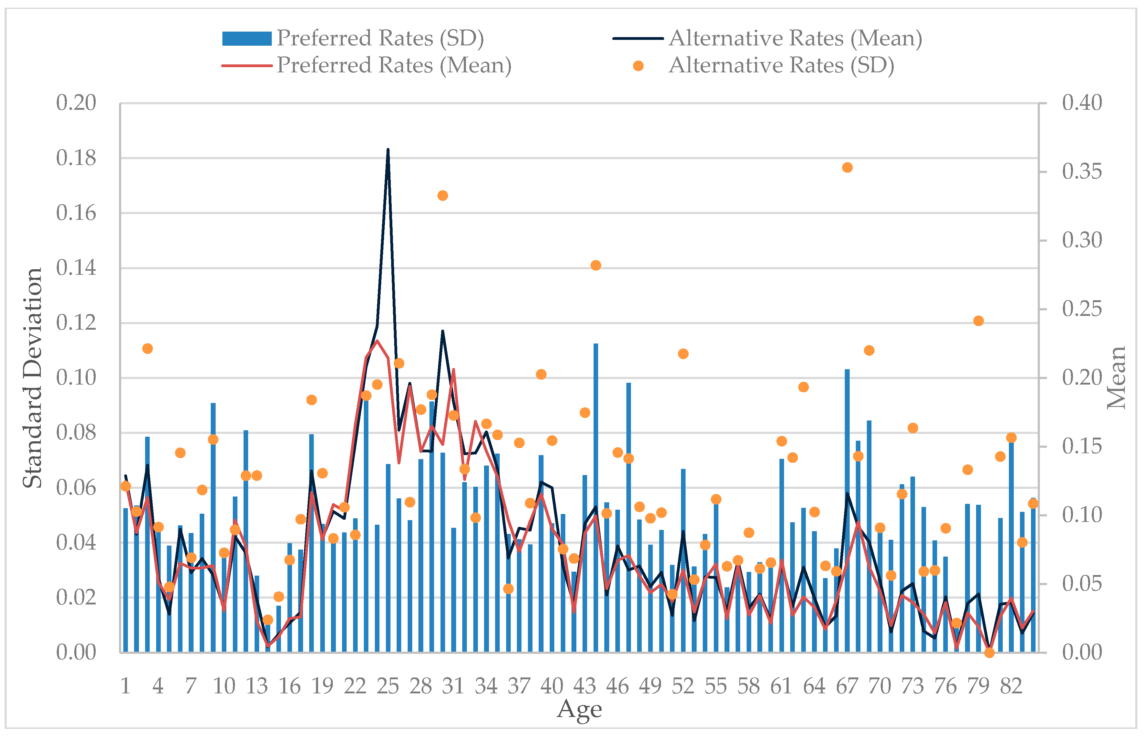
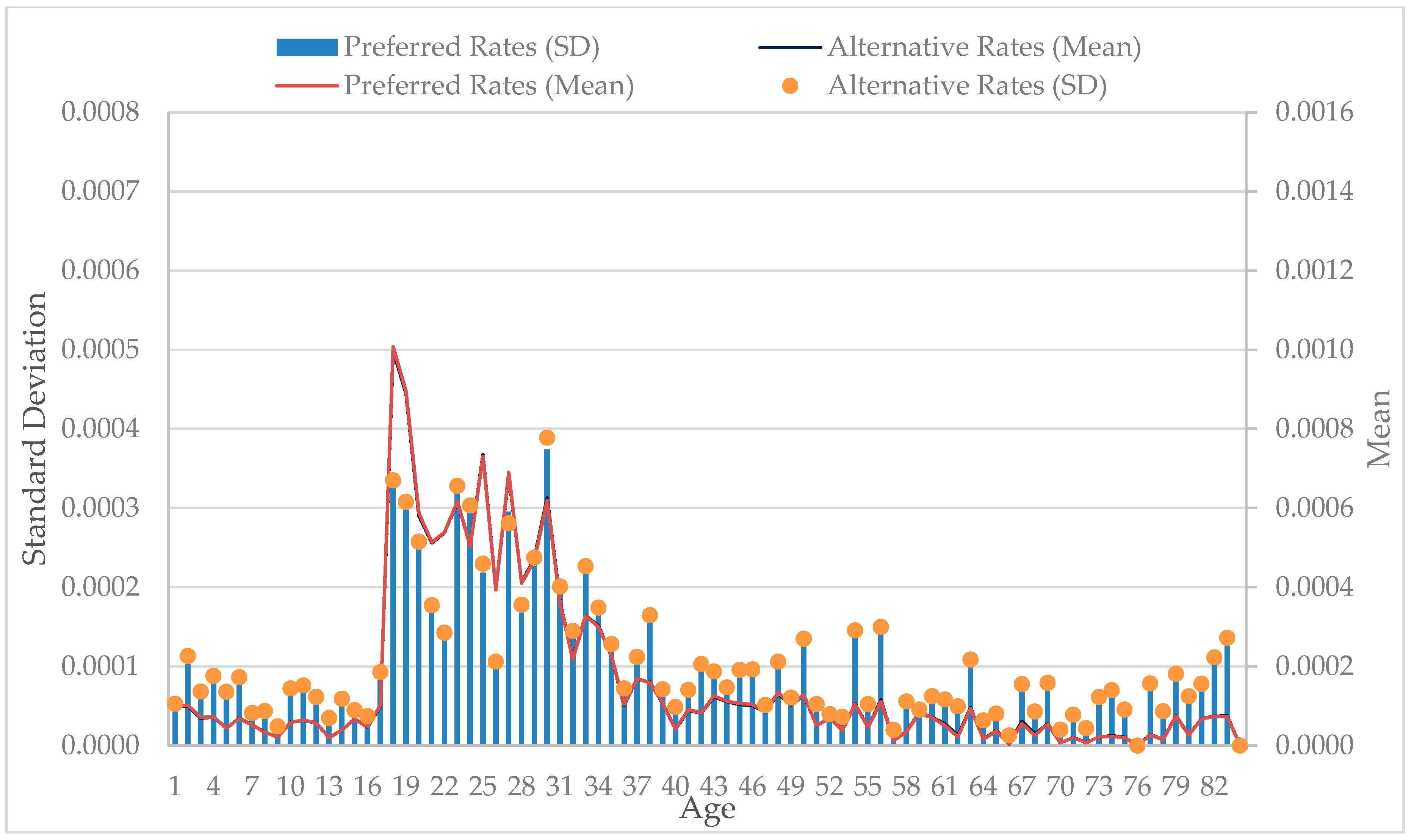
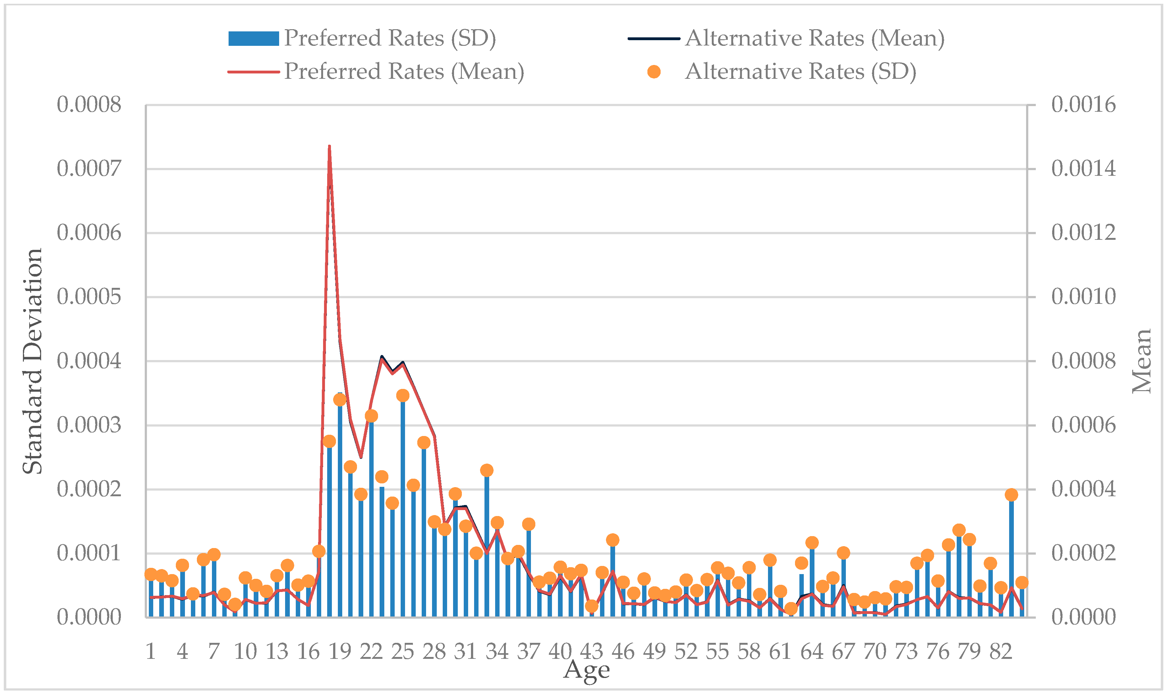
Standard deviations were lower for our preferred synthetic estimators that better identified the population at risk of migrating using one ACS sample (Equations (1) and (2)) than those using two ACS samples (Equations (3) and (4)). Figure 1, Figure 2, Figure 3 and Figure 4 present the standard deviations of our preferred rates from 2007 to 2014, with synthetic population denominators represented by a bar and standard deviations using the alternative rates from two samples represented by a point. In Figure 1 and Figure 2 for males and females, 62.6 percent of single-year age domestic out-migration rates (105 of the 168 single-year ages) had lower standard deviations for the preferred rates compared to the alternative rates. Our preferred domestic in-migration rates in Figure 3 and Figure 4, with the United States synthetic population in the denominator, saw a smaller improvement over the alternative population estimation. A slightly increased share (51.8 percent) of single-year age domestic in-migration rates (87 of the 168 single-year ages) had lower standard deviations for the preferred rates compared to the alternative rates. These results suggest we gained efficiency by using our preferred estimator, especially for domestic out-migration.
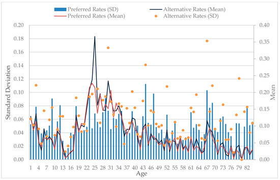
Figure 1.
Means and Standard Deviations of Male Domestic Out-Migration Rates, 2007–2014. Source: 2006–2014 1-Year American Community Survey.
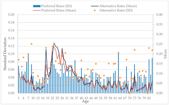
Figure 2.
Means and Standard Deviations of Female Domestic Out-Migration Rates, 2007–2014. Source: 2006–2014 1-Year American Community Survey.

Figure 3.
Means and Standard Deviations of Male Domestic In-Migration Rates, 2007–2014. Source: 2006–2014 1-Year American Community Survey.

Figure 4.
Means and Standard Deviations of Female Domestic In-Migration Rate, 2007–2014. Source: 2006–2014 1-Year American Community Survey.
The migration rates in Figure 1, Figure 2, Figure 3 and Figure 4 conformed to our expectations about Boston’s age structure and supported the decision not to use smoothing techniques. In-migration peaks at age 18 due to college enrollment and slows after college but remains elevated until age 35. Out-migration also peaks around the college years. With this clear pattern, any smoothing technique could alter migration for adjacent ages. For example, migration of 17-year-olds who are enrolled in high school should not be inflated by any smoothing technique related to the migration of college students. This method transparently matches the single-year age migration pattern for Boston related to college enrollment. The projection keeps Boston’s unique age structure, as it projects the city’s 2030 and 2035 populations with a slightly aging population, while keeping the increased population due to college enrollment.
Our 1-year migration rates with synthetic populations were efficient, but they still had large standard errors. After calculating these 1-year migration rates from each ACS year between 2007 and 2014, we chose to temporally aggregate the age and sex-specific migration rates to reduce the effects of sampling error. We chose the temporal aggregation method over regional and family membership methods [17]. As shown in Figure 1, Figure 2, Figure 3 and Figure 4, Boston’s population structure is shaped by migration patterns over time: Migration from Boston in the early years of life, followed by rapid migration to Boston between ages 18 to 24, and then gradually decreasing migration from Boston. These age-specific patterns were likely to dominate over time, so averaging across a number of successive years should help increase the reliability of age and sex-specific migration rates. These averaged single-year age rates were operationalized into 5-year rates needed for our projection methodology.
To further compare the efficacy of our preferred migration rates, we applied both rates in different interregional cohort-component models to assess how well each projected Boston’s 2015 population. The U.S. Census Bureau provides several estimates for Boston’s population. As previously mentioned, the ACS estimate for Boston in 2015 was 669,496 ± 2608. The Census Bureau’s PEP provided three estimates for 2015: Vintage 2015, 667,137; Vintage 2016, 665,984; and Vintage 2017, 669,255. These PEP estimates provided a July 1st point estimates for Boston’s population that used administrative and not survey data to estimate Boston’s population. Table 1 reports PEP and ACS and 2010 Census estimates to assess the forecast accuracy from our preferred (666,261) and alternative (650,947) projections for Boston in 2015. If the population estimate and projection matched, the forecast error would be 0. For example, the 2015 population growth from the 2010 Decennial Census to the Vintage 2017 population estimate was 51,661 and population growth of the preferred population projection was 48,667, and the forecast error was 2994 fewer people projected by our model than the Census Bureau estimate. This represented −5.8% of the growth from the Vintage 2017 population estimate for Boston in 2015.

Table 1.
Comparison of Residual Population Change by Program for Boston 2010–2015.
We compared our alternative and preferred projections to several 2015 U.S. Census Bureau estimates for Boston in Table 1. Our preferred projected population for Boston was 666,261 and our alternative population projection was 650,947. When comparing our two projections to the PEP and ACS estimates, our preferred projection consistently projected Boston’s population more accurately than our alternative projection without synthetic population estimates.
4. Discussion
Although gross migration is a preferred measure of migration [1,2,3,4], we had to overcome data limitations in developing an interregional cohort-component projection methodology. In the United States, the ACS measures migration, but may not have the needed statistical power for generating reliable migration rates for smaller regions. This research describes an innovative method to generate efficient migration rates with synthetic populations from a series of single-year ACS samples that clearly identified the population at risk of domestically migrating to and from Boston. The at-risk population was a synthetic population identified in each ACS sample. These people are living in Boston the year when the migration occurred for domestic out-migration rates, and people living in the United States outside of Boston the year when the migration occurred for domestic in-migration rates. For example, when the age-specific migration rate is the number of females who migrated at age 30–34 in one ACS, then the denominator is the number of females 30–34 years of age in the same sample; only they are at risk of becoming 30–34 year old migrants. Connecting migration and population data in one survey met the requirement of the at-risk principle of demography for creating migration rates. The numerator and the denominator of each domestic migration rate match, and these rates are probabilities that the migration will occur for the members of a specific cohort. These innovative rates projected Boston’s population closer to the 2015 U.S. Census Bureau estimate than a projection using an ACS population estimate from the year prior to the migration to calculate migration rates. This innovation increased the validity of ACS migration data to generate migration rates.
In developing these migration rates, we successfully addressed weaknesses in the ACS [13] for regions with smaller populations by generating efficient synthetic populations in relation to migration data [18]. The domestic migration rates with synthetic populations were more efficient compared to rates using two ACS samples. Due to Boston’s unique age structure, this method was preferable to others using smoothing techniques [17]. Other regions without a special population like college students might prefer using smoothing techniques with our alternative rates. However, this method would not directly match the right rates to the right people surveyed for Boston [5]. By creating synthetic populations and aggregating eight years of data [15], we identified the population at risk of migrating, reduced the standard errors of the migration rates, and produced more reliable rates. Using these rates, our model better projected Boston’s 2015 population than a model using actual ACS population estimates to generate migration rates.
Our method of creating synthetic populations to generate migration rates from one survey year and aggregating samples are transferable to any similar survey data containing domestic in- and out-migration estimates. Application of this method to other areas should examine the statistical power of the survey data to provide the necessary statistical confidence. In our example, ACS data were available only for a region with a population of at least 100,000, and the aggregated sample required approximately 42,000 observations for a region the size of Boston. This data limitation reduces the generalizability of this method to other smaller regions, but increasing the sample to include a longer time interval could reduce this limitation [13]. Further research is needed to evaluate the efficacy of this method for using more years of migration data in regions with smaller populations.
Reliable intercensal domestic migration rates for smaller regions like Boston are needed because projection models using net migration may not project the age structures of a region with special populations as well as those using gross migration [4,5,10]. Our projection methodology needed to use single-year age migration rates identifying the right at-risk population because of Boston’s migration related to college students [5,7]. By more accurately estimating migration rates for this cohort with increased levels of migration, we more accurately projected Boston’s 2015 population.
This population projection was needed because the U.S. Census Bureau was estimating more rapid population growth for Boston, and projections using a vital statistics methodology could not reliably be generated until the release of the 2020 Census. Identifying this at-risk synthetic population allowed us to use a preferred interregional projection model that has been shown to better project the population than a projection model using net migration [4,5,10]. These projections contributed to long-term planning for Boston’s housing and education departments, with their need to identify future targeted housing production and projected school enrollment. Identifying changes in the population due to college enrollment was important for this future planning. This allowed for more ease in interpreting these results for planning the city’s future development. Future research is needed to allocate this projected population to Boston’s neighborhoods to provide a more granular perspective on population growth to inform city planning.
This practice-oriented, cohort-component research attempts to serve as a guide to and encourage discussion of projection methods, especially in light of the dependency upon ACS data in the United States [5]. Our use of ACS data to create synthetic populations to generate migration rates is a practical way to address fluctuations in 1-year migration data that exists in regions with smaller populations while adhering to the at-risk principle of demography. More complex fitted models and those using smoothing techniques have been developed to adjust ACS data to address this variation [17], but simpler models often project the population more accurately than complex models [16]. The methodology we have described here transparently estimates 1-year migration rates with minimal assumptions and can be implemented by data analysts with basic statistical software packages.
Author Contributions
P.G., C.K. and M.R. conceived and designed the migration rates; P.G., C.K., J.L., A.L. and M.R. analyzed the data; K.K. developed the analysis tools; P.G., C.K. and M.R. wrote the paper.
Funding
This research received no external funding.
Acknowledgments
We would like to thank Tim Reardon and Meghna Hari of the Metropolitan Area Planning Council for their comments on earlier versions of the migration rates. In addition, we thank three anonymous reviewers for their comments to a previous version of this manuscript.
Conflicts of Interest
The authors declare no conflict of interest.
References
- Rogers, A. Matrix methods of population analyses. J. Am. Inst. Plan. 1966, 32, 40–44. [Google Scholar] [CrossRef]
- Hightower, H.C. Population Studies. In Principles and Practices of Urban Planning; Goodman, W.I., Freund, E.C., Eds.; International City Mangers’ Association: Washington, DC, USA, 1968. [Google Scholar]
- Rogers, A. Regional Population Projection Models; Sage: Beverly Hills, CA, USA, 1985. [Google Scholar]
- Rogers, A. Requiem for the net migrant. Geogr. Anal. 1990, 22, 283–300. [Google Scholar] [CrossRef]
- Isserman, A.M. The right people, the right rates: Making population estimates and forecasts with an interregional cohort-component model. J. Am. Plan. Assoc. 1993, 59, 45–64. [Google Scholar] [CrossRef]
- Isserman, A.M.; Plane, D.; McMillen, D. Internal migration in the United States: An evaluation of federal data. Rev. Public Data Use 1982, 10, 285–311. [Google Scholar]
- Plane, D.A. Demographic influences on migration. Reg. Stud. 1993, 27, 375–383. [Google Scholar] [CrossRef] [PubMed]
- Smith, S.K. Accounting for migration in cohort-component projections of state and local populations. Demography 1986, 23, 127–135. [Google Scholar] [CrossRef] [PubMed]
- Smith, S.K.; Swanson, D.A. In defense of the net migrant. J. Econ. Soc. Meas. 1998, 24, 249–264. [Google Scholar]
- George, M.V.; Smith, S.; Swanson, D.A.; Tayman, J. Population projections. In The Methods and Materials of Demography, 2nd ed.; Siegel, J.S., Swanson, D.A., Eds.; Elsevier Academic Press: San Diego, CA, USA, 2004; pp. 561–602. [Google Scholar]
- Citro, C.F.; Kalton, G. Using the American Community Survey: Benefits and Challenges; National Academies: Washington, DC, USA, 2007. [Google Scholar]
- Isserman, A.M. The accuracy of population projections for subcounty areas. J. Am. Inst. Plan. 1977, 43, 247–259. [Google Scholar] [CrossRef]
- Rogers, A.; Jones, B.; Ma, W. Repairing the Migration Data Reported by the American Community Survey; Working Paper POP2008-01; Institute of Behavioral Science—Population Program: Boulder, CO, USA, 2008. [Google Scholar]
- Beaumont, P.M.; Isserman, A.M. Comments on tests of accuracy and bias for population projections. J. Am. Stat. Assoc. 1987, 400, 1004–1009. [Google Scholar]
- Smith, S.K.; Sincich, T. The relationship between the length of the base period and population forecast errors. J. Am. Stat. Assoc. 1990, 85, 367–375. [Google Scholar] [CrossRef] [PubMed]
- Rogers, A. Population forecasting: Do simple models outperform complex models? Math. Popul. Stud. 1995, 5, 187–202. [Google Scholar] [CrossRef] [PubMed]
- Rogers, A.; Little, J.; Raymer, J. The Indirect Measure of Migration; Springer: New York, NY, USA, 2010. [Google Scholar]
- Smith, S.K.; Tayman, J.; Swanson, D.A. A Practitioner’s Guide to State and Local Population Projections; Springer: New York, NY, USA, 2013. [Google Scholar]
- Wetrogan, S. Projections of the Population of States, by Age, Sex, and Race: 1988–2010; Current Population Reports, P-25, No, 1017; Census Bureau: Washington, DC, USA, 1988.
- Campbell, P.R. Population Projections for States by Age, Sex, Race and Hispanic Origin: 1995 to 2050; PPL47; Census Bureau: Washington, DC, USA, 1996.
- Smith, S.K.; Rayer, S. Projections of Florida Population by County, 2015–2040, with Estimates for 2012; Florida Population Studies, Bulletin 165; Bureau of Economic and Business Research, University of Florida: Gainesville, FL, USA, 2013; Volume 46. [Google Scholar]
- Wonnacott, T.; Wonnacott, R. Introductory Statistics; John Wiley & Sons: New York, NY, USA, 1990. [Google Scholar]
- Seltman, Howard. Approximations for Mean and Variance of a Ratio. Available online: http://www.stat.cmu.edu/~hseltman/files/ratio.pdf (accessed on 30 November 2017).

© 2018 by the authors. Licensee MDPI, Basel, Switzerland. This article is an open access article distributed under the terms and conditions of the Creative Commons Attribution (CC BY) license (http://creativecommons.org/licenses/by/4.0/).