Abstract
Currently, more than half of the world’s population lives in cities. Out of these more than four billion people, almost one quarter live in slums or informal settlements. In order to improve living conditions and provide possible solutions for the major problems in slums (e.g., insufficient infrastructure), it is important to understand the current situation of this form of settlement and its development. There are many different models that attempt to simulate the development of slums. In this paper, we present data mining models that correlate information about the temporal development of slums with other economic, ecologic, and demographic factors in order to identify dependencies. Different learning algorithms, such as decision rules and decision trees, are used to learn descriptive models for slum development from data, and the results are evaluated with commonly used attribute evaluation methods known from data mining. The results confirm various previously made statements about slum development in a quantitative way, such as the fact that slum development is very strongly linked to the demographic development of a country. Applying the introduced classification models to the most recent data for different regions, it can be shown that the slum development in Africa is expected to be above average.
1. Introduction
Urbanization is one of the greatest challenges faced by humanity in the coming years. As of 2007, more than half of the world’s population lives in cities, and this proportion is expected to increase even further in the future [1]. In particular, cities in the Global South (Africa, Asia, and South America) are characterized by a rapidly increasing number of inhabitants, creating considerable problems for the infrastructure in the respective cities [2]. These problems are particularly evident in so-called “slums”, in literature often referred to as “informal settlements”. There are many discussions in the literature about these terms and the transferability of definitions to different regions (cf. Hofmann et al. [3]). In this context, we generally speak of settlements of the urban poor [4,5]. According to the United Nations (UN), “a slum household is defined as a group of individuals living under the same roof lacking one or more of the following conditions: access to improved water, access to improved sanitation, sufficient living area, and durability of housing” [1]. In this paper, we investigate “slums” (according to the definition of the UN), knowing that the morphology and structure of these settlements can be very different worldwide [6]. The UN estimates that about one billion people worldwide currently live in slums. This number is expected to double or even triple by 2050 [7]. These settlements are often undersupplied in terms of water, energy, and sanitation, which leads, among other things, to an increased mortality rate among children, as well as negative consequences for the mental and physical health of the residents [8,9,10]. Therefore, it is very important to improve the living conditions of these people. This objective has consequently been included in the UN’s global goals for sustainable development. For this purpose, it is important that we gain an understanding of slums and their development. Slums have been studied in the literature in many ways. In different qualitative studies, aspects of the life of the residents such as health [11], sexual behavior [12], living situations [13], and their connections [14] have been examined in different ways. It is necessary to collect information about slums and to analyze possible reasons for slum development to identify future scenarios and create holistic solution strategies [15,16] to solve the problems related with these settlements. Identifying factors that correlate with strong slum growth can help us to understand the underlying processes of slum growth better.
In the literature, many different factors have been described which were identified as leading to slum development. Mahabir et al. [17] mention four factors influencing the growth of slums. These are (i) location choice factors; (ii) rural-to-urban migration; (iii) poor urban governance; and (iv) ill-designed policies. Roy et al. [18] define the following seven factors: population dynamics, economic growth, housing market dynamics, informal economy, local topography, street pattern, and the politics of slums. While some of these previously mentioned factors primarily relate to local conditions (e.g., streets or local topography), others have economic and demographic roots. Current methods of slum modeling follow a bottom-up approach. They are mostly agent-based or work with geographic information systems, like the informal settlement growth model [19] or slumulation [20]. A detailed review of these models can be found in Roy et al. [18].
In contrast, this work attempts to investigate slum development based on country-level information [21]. We use data mining methods to analyze to what extent economic, demographic, and other factors correlate with slum development, and how the development can be validated quantitatively. Thus, we address the following research question in this paper:
RQ:Which national indicators correlate with a high growth of urban slum population?
To answer this question, we apply commonly used data mining methods to data taken from the World Development Indicators (WDIs ) of the World Bank [22], which has been collecting a large number of indicators annually from various sources.
Data mining methods have been frequently used in slum research in the context of remote sensing, as shown by detailed reviews [23,24]. Several studies have also investigated the correlation between the proportion of the urban population living in slums with other factors, such as infant mortality [25] or CO2-emissions [26]. The World Development Indicators provided by the World Bank have often been used as a database in these studies [22]. However, no study is known to examine the World Bank data set as a whole using data mining methods to investigate relationships between the growing number of slum dwellers and other factors.
The procedure to address the research question is as follows: After introducing the used data set (Section 2.1), we briefly describe the framework applied within this work (Section 2.2), then present the methods of machine learning and evaluation used for the survey (Section 2.3). After presenting the results of the study (Section 3), we finally discuss these results (Section 4) and close with an outlook on possible future work (Section 5).
2. Materials and Methods
Within this section, we first describe the dataset used for our study as well as the general framework, and then explain the applied data mining methods.
2.1. Overview on Data Set and Pre-Processing
To conduct our study, we use the WDI dataset [22] provided by the World Bank. This data set comprises data collected by the World Bank from official international sources since 1960. It includes 1453 indicators about agriculture, economics, health and demography, education, infrastructure, and more for 217 countries and economic zones. All indicators mentioned in this work are listed in Appendix B, with their respective category. We carried out the categorization based on the World Bank categorization. Information on the sources of each indicator can be found in Reference [22]. A regional breakdown of the included countries can be found in Table 1. Since one of these indicators quantifies the proportion of the urban population living in slums, we can use this data set to derive the temporal development of the population living in slums and find correlations to other variables provided in the data. The WDIs use the data on the percentage of urban slum population provided by the UN-Habitat [22]. To get detailed information on the underlying processes of slum growth, investigating data at the city level leads to more accurate results. The use of data at the national level blurs information, as this approach combines the data of different cities in the same country with possibly different characteristics. However, we used the data of the World Development Indicators, which are only available at the national level, because they provide a very comprehensive set of many different indicators at a global scale. The methods presented here could also be applied if there were sufficient data available at the city level, and the results of both investigations could be compared.

Table 1.
Regional breakdown of the analyzed data [22].
Although the dataset includes data for every year, information about the proportion of urban population living in slums is only available for the years 1990, 1995, 2000, 2005, 2007, 2009, and 2014. Moreover, the information is only available for up to 106 countries, and even for these countries the information is not available for all of the above-mentioned years. In total, we have 436 data points with information about the slum population of a country at a specific point in time. The proportion of the urban population living in slums varies between 3 and 97 percent. For all of these data points, additional information relating to other indicators is available. The data are included in a table, and the different data points can be identified by country and year. An exemplary extract of the dataset is shown in Table 2.
Table 2.
Excerpt of the used data set [22].
Since we wanted to analyze the development of the slum population based on static data, we had to perform some preprocessing. We calculated the absolute number of inhabitants of these slums:
using the total urban population and the percentage of the slum population from the urban population.
Having calculated this value for the same country for two points in time “now” and “later”, we indicated the relative development of the number of inhabitants between the two times as:
If we, for example, wanted to analyze the instance of Afghanistan in 2000, we would take all indicators measured in the year 2000 and additionally calculate the slum development from 2000 to 2010 (if the timestep was 10 years). This greatly reduces the number of instances that can be included in the data mining analysis since we need two data points on the slum population from the same country at a fixed timestep. Once we calculated slum developments of all available n countries for a given timestep, we calculated the average growth:
We did not use this directly as our target variable. While there are decision tree learning methods available that can handle numerical target values [27], the training of non-linear non-parametric regression models typically requires a larger number of training examples than were available for our task. For this reason, we decided to discretize the target variable by forming two classes: one for above-average slum growth () and one for below-average slum growth (). We also considered splitting the data based on the median, which would yield a perfectly balanced set except in cases where many countries have the same growth value. However, the differences were negligible in this case. This binary specification was our target attribute for the analysis. Defining a two-class problem in this way has the key advantages that the classes are comparably balanced. That is, both have approximately the same number of instances and the results are relatively easy to interpret.
2.2. Framework
The framework of this paper is illustrated in Figure 1. In order to learn models that allow discrimination between above-average and below-average slum development, we applied three commonly used classification methods to the data set described above—the random forests ensemble classification method [28], the rule learner “ripper” [29], and the decision tree learner C4.5 [30]—in their implementations available in the Weka Knowledge Acquisition workbench [31,32]. Since Weka is an open source platform, the described approach can be applied to the presented data or other data by other researchers. We also conducted different types of attribute evaluation to identify factors that had a high influence on this discrimination [33], evaluate the different results, and compare them quantitatively. In this context, it is also important to note that the methods presented only identify correlations and links between the growth of slum population and the other different indicators. Our goal in this study was not to establish causal relationships between different indicators and slum growth, but to identify and quantify them.
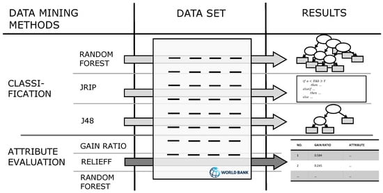
Figure 1.
The framework of our research approach. The different methods will be introduced in the following Section 2.3.
2.3. Machine Learning Methods
Methods and algorithms in the field of data mining aim to discover knowledge from structured data [34]. Data are usually represented with a set of independent variables (often referred to as attributes), and a singled-out dependent variable—the so-called class or target variable. Knowledge consists of frequently re-occurring patterns and regularities in a set of given examples—the so-called training instances. Detected regularities should not only hold true for the data at hand, but also apply to other unseen instances drawn from the same distribution. To achieve this, it is typically not sufficient to find patterns that perfectly fit to the given data, but to instead take minor deviations into account, with the goal of finding a simpler model that typically yields better predictions. This avoidance of overfitting is a very general principle in machine learning, which is known under various names such as pruning or regularization [35]. Different algorithms employ different approaches to incorporating such a generalization bias, and may consequently yield different models, which nevertheless often exhibit similar predictive behavior.
In this paper, we focus on two model types, decision trees and classification models, which are different ways of formulating logical rules. However, it should be noted that the resulting rules must not be interpreted as causal models, but should rather be seen as multi-dimensional correlations. Thus, we will focus our interpretations not so much on the concrete rules and trees that have been learned, but on the attributes that have been used in these models. We therefore also employ attribute evaluation methods, which help to determine the most important factors that influence the target value. The used methods are summarized in Figure 1, and are described in more detail below.
2.3.1. Classification Methods
Algorithms for classification observe how a particular attribute, called the target attribute, behaves depending on the remaining attributes. On this basis, models are learned which can subsequently be used to assign a value for the target attribute to previously unseen instances. This process is called classification. This work uses the standard implementations of common algorithms in the WEKA framework [31,32], which were designed to find the best models for the classification process. These models were then evaluated and interpreted. We selected two types of algorithms: the rule learning algorithm JRip, and the decision tree learner J48. Both algorithms are well-known and frequently used in machine learning and data mining. Although they essentially solve the same task (i.e., finding a declarative prediction model for a target variable), they can provide different solutions. On the one hand, the algorithms differ in the way the relationships between the individual attributes are recognized, and on the other hand in the type of models they provide as results.
JRip
JRip is the WEKA implementation of the rule learning algorithm ripper [29], which creates a model in the form of a list of rules. Rules are particularly interesting for such analyses because they can typically be interpreted directly by domain experts without a strong background in machine learning or computer science [36]. A rule consists of the body of the rule (the IF-part), which states a number of conditions that have to be met before the conclusion of the rule (the THEN-part) can be applied. In our case, the conditions were conjunctions of specific values for the input variables (characteristics of individual countries), and the conclusion part was a prediction for the target variable (i.e., for the future slum development). To classify an instance, rules are consulted from top to bottom to determine whether all the conditions of the IF branch of the rule are satisfied. If this is the case, the target attribute is set to the value specified in the conclusion. Otherwise, the IF branch of the next rule is considered. The list of rules is typically terminated with a default rule (an ELSE-branch). This default rule consists of a prediction for cases in which the conditions of no other rule are met.
J48
J48 is a decision tree learner based on the classical C4.5 algorithm [30]. Unlike rule learning algorithms, which learn lists or sets of rules, decision tree learning algorithms build up a tree-based decision model. Typically, this model has the more important decision variables near the top of the tree (its so-called root), due to the way the algorithm builds the tree. Starting at the root, all possible variables are evaluated at any node, and the algorithm selects the node which provides the best separation with respect to the target variable. This is repeated recursively, until a node is reached that only contains examples which share the same value for the target variable. Then, a so-called leaf node is added to the tree, which recommends this value as suitable for all examples that arrive at this node (i.e., which follow the same path from the root to this leaf). To classify an instance with this model, the tree is followed from top to bottom, whereby the attribute value of the instance to be classified always determines which path is chosen . This is repeated until a leaf node is reached which specifies the recommended classification decision.
Random Forests
Rule learning and decision tree learning algorithms focus on learning interpretable models, but sometimes the prediction quality is higher for models which are not directly interpretable. One example of this is ensemble methods, which learn multiple different models and make a final prediction by taking a majority vote on their predictions. Particularly effective and commonly used ensemble methods are random forests, which learn multiple trees from a single dataset [28]. To make the trees differ, they use different subsets of the attributes and train on different subsets of all instances, but always have the same target attribute. Since random forests containing a hundred decision trees are used in the work, the individual trees are not mapped or interpreted. However, random forests can on the one hand give a better estimate of an achievable model quality, and on the other hand are well-suited for the evaluation of attributes, since one can observe how often individual attributes were used for the tree structure and how effectively they contributed to the classification in the respective tree.
2.3.2. Evaluation Methods for Predictive Data Mining
In order to evaluate the quality of the learned model, machine learning typically does not rely on methods that are used in descriptive statistics (e.g., correlation between the model and the target values), but have developed methods that particularly aim at evaluating the quality of the found model on potentially unseen data.
The most commonly used method in machine learning is k-fold cross-validation [37], which divides the instances into k sets of equal size, typically using stratified sampling. All k sets are used once as a test set to test the model that was trained on the remaining sets. In this way, exactly one out-of-sample prediction is returned for every available example.
The larger the value of the parameter k that is selected, the more independent the overall result is of the individual divisions into learning and test sets, but the more expensive the evaluation becomes because more models have to be learned and evaluated. A commonly used value is [38], which is also used in this work. In a 10-fold cross- validation (10-CV), each instance is therefore used 9 times to build a model, and all 10 models are evaluated independently of each other. Since each instance was classified exactly once as part of a test set, the results of the individual evaluations can be summarized.
Another version of cross-validation in which k is selected to a maximum size (i.e., where n is the number of instances) is known as leave-one-out cross-validation, sometimes also referred to as the jackknife. In this case, a separate model is built for each instance by using all other instances as a training set and is then evaluated using only this instance as a test set.
In our work, we developed a slightly modified strategy called leave-one-country-out (LOCO), which creates one set for all instances of the same country. The underlying idea behind this method is that instances from the same country differ only marginally at different times, such that the results of a conventional cross-validation, which would randomly distribute different instances originating from the same country over the training and test sets, might yield overly optimistic evaluation estimates because instances from the same country can be found in both the training and test sets. Leaving all instances of one country out avoids this problem, and repeating this for each country also guarantees that exactly one out-of-sample prediction is obtained for each point in the original dataset. In order to evaluate the algorithms with this evaluation method, a function of the WEKA-API was adapted accordingly.
The evaluation of a model thus describes the learnability of a data set from the given algorithm, and is a yardstick for how precisely the final model can classify new, unseen instances (i.e., countries). However, it is important to note that the individual folds of the cross-validation are not interpreted or used otherwise. They only serve the purpose of jointly delivering a quality estimate for a single model that is trained on the entire instance set, which is the final output of the learning algorithm.
2.3.3. Attribute Evaluation
In addition to learning complete prediction models, we also aimed at identifying attributes that correlate well with significant growth in slum populations. To do so, we tested three different methods that operate on different levels. The first, information gain ratio, treats every attribute in isolation and correlates its value with the target variable. The second method, ReliefF, takes the immediate neighborhood, and thus the discriminatory power of each attribute, into account. As already mentioned, the third evaluates an attribute based on the frequency with which it is used in a random forest classifier.
Information Gain Ratio
The information gain ratio criterion is frequently used for attribute evaluation in machine learning. It essentially estimates the information gained about the target value when the value of the attribute is known. However, such estimates of mutual information tend to be higher for attributes with a high number of values, so the term is normalized with the maximum entropy reduction possible with this attribute [39]. Its use here may be viewed as a conventional statistical correlation measure, indicating that attributes with higher information gain ratio carry more information about the target value. There are many other possible choices which would yield similar results. We decided to use this because it is also used in the decision tree and (in slightly modified form) in the rule learning algorithms, where it is used for composing more complex multi-variable models that can capture non-linear interactions of multiple attributes with the target value.
ReliefF
The Relief method [40] and its successor ReliefF [41] rate attributes highly that have the following properties:
- Similar instances with the same class have similar attribute values;
- Similar instances with different classes have different attribute values.
To achieve these objectives, it computes a weight for each feature which essentially estimates the probability difference between the occurrence of a near hit (an instance of the same class) and a near miss (an instance of a different class) in the vicinity of an example defined by the attribute in question.
Random Forest Evaluation
As already described above, the random forest algorithm creates several decision trees, each with a subset of all available attributes.
Starting from the root, the trees select the attribute that has the highest information gain ratio for the instances occurring in the subtree that starts in the current node. Therefore, the information on how often an attribute was used by all decision trees in the entire ensemble is a good indicator of whether an attribute correlates well with the target attribute on different subsets of all instances. In addition to the flat analysis, which is provided by information gain ratio and treats every attribute in isolation, this technique will also take into account how important an attribute is in relation to the other attributes in a dataset.
Typical measures that capture this information are how often the attribute was used in the individual trees of the forest, or the average reduction of entropy that is obtained by the use of this attribute. The use of random forests for attribute evaluation has already been proposed by Breiman [28], and has since been used in various applications (e.g., [42]).
3. Results
We describe the results of our study in the following section. We first present two models for a timestep of 10 years, followed by the evaluation results for the three investigated classification methods. Furthermore, we describe the main findings of the learned models. Afterwards, we show indicators with a high correlation to slum development based on the three different approaches to attribute evaluation.
3.1. Classification Models for Slum Development for a Timestep of 10 Years
When looking at the model found with J48 for a timestep of 10 years (Figure 2), the first and second nodes contained demographic aspects, like the proportion of the population with ages between 0–14 and the total urban population. A high proportion of young people (more than 41.43 percent) correlated with a slum growth higher than average. If the proportion of young people was below the threshold mentioned above, the next node was to use the total urban populations as a decision criterion. The last two nodes were economic indicators. The import value index “is the current value of imports (c.i.f.) converted to U.S. dollars and expressed as a percentage of the average for the base period (2000)” [22]. If this value was below 238.6, the slum growth was classified as lower than average. If it was above, the last decision criterion was the value of the adjusted net savings. For detailed information on the indicators, please see [22].
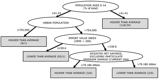
Figure 2.
The model found with J48 for a timestep of 10 years.
In comparison to this J48 model, the model found with JRip was quite simple (cf. Decision Rule 1). The only decision criterion was the “Fertility rate”. If it was higher than 5.15, the slum development was higher than average, if it was below this value, the slum development was lower than average. Even though this did not yield a perfect discrimination yet, additional factors were not considered to deliver further improvements in the prediction quality of the found rules.
| Decision Rule 1: Result for JRip for 10 year timestep. |
 |
3.2. Analysis of Slum Development
Table 3 shows information about the data set as well as the results of the attribute evaluation. The number of available instances decreased with increasing timesteps. It can also be seen that the total number of slum dwellers within a country almost doubled within 20 years.
Table 3.
Evaluation of the different classification methods for predicting slum growth over different time spans. 10-CV: 10-fold cross-validation ; LOCO: leave-one-country-out.
The results showed that the prediction accuracy of the different algorithms, measured as the share of instances classified correctly, varied between 68% and 84%. All learned models were clearly better than guessing of the largest class, which would have yielded only about 55% prediction accuracy, since the larger class had 55% of all instances (the exact values for each data set can be found in the fourth row of the table). We can also see that the random forest algorithm yielded the best results for all timesteps and both evaluation methods.
Comparing the evaluations in Table 3 for the different models, the prediction accuracy differed only minimally for the different timesteps. It was equally possible to determine whether a slum will grow at an above-average rate in 5 years or at an above-average rate in 20 years. However, the prediction models tended to become simpler, which became visible in various parameters that characterize the complexity of the learned models, such as the number of rules, the average number of conditions per rule, the number of nodes in a decision tree, or the maximum depth of the tree. The learned models for the timesteps of 5 and 20 years can be found in Appendix A.
While the prediction for the five years has to distinguish many cases (several long rules or a larger number of nodes), in the long run (10 and 20 years) only a few factors are decisive for slum growth. This corresponds with few, short rules or a small number of nodes in the trees. Examining the determining attributes of the models (Section 3.1 and Appendix A), we find strong similarities. The largest groups were demographic attributes such as “Population ages 0–14”, “Urban population growth”, “Fertility rate”, etc. All three trees had the attribute “Population ages 0–14” as root nodes, and used this first query to assign a class directly to a subset (i.e., on one side the tree ended with a leaf and its related classification directly below the root). The thresholds of the decision variables were also similar and just over 40 percent. The rule set (JRip) for 10 years even consisted of only one rule with the attribute “Fertility rate”. There were also economic and agricultural factors, such as the “Crop Production Index”, “Import Value Index” and “Final Consumption Expenditure”, which often form a rule with demographic attributes or occur in subtrees caused by them. In addition, health problems (e.g., “Lifetime risk of maternal death”) occured as a factor.
3.3. Indicators with High Correlation to Slum Development
While the models shown above (Section 3.1) give plausible explanations for slum growth and the opportunity to interpret the emergence of certain attributes, they do not provide a complete overview of the correlation ratio between each individual attribute and the target attribute. For this reason, we used the attribute evaluation algorithms presented in Section 2.3.3 to evaluate the attributes according to their influence on certain questions.
In addition to information gain ratio, we also examined the correlation with the target attribute “slum development above or below average within 5 years” using the evaluation functions ReliefF and random forest evaluation.
3.3.1. Information Gain Ratio
The results for the information gain ratio evaluation are shown in Table 4.
Table 4.
The five attributes with the highest information gain ratio for forecasts over three different time spans.
For all three timesteps—5, 10, and 20 years—the top five attributes were almost exclusively related to demographic characteristics. It can be seen that the composition of the population from different age groups had a very large influence on whether the slum development was above or below average. Even if the information gain ratio values did not give us a formula for the type of influence, we can see from the models shown in the Appendix A how the attributes influenced the slum development. Thus, we see that “Population ages 0–14” above approx. 41% led to a classification for a slum development “higher than average” in all three decision trees. In addition, the information gain ratio increased by up to 50%, but at least by 30%, when jumping from 10 to 20 years. This explains why our models were able to keep the prediction accuracy at 80% with fewer rules/nodes. This increase was also visible in the prediction accuracy of the root nodes (Appendix A). For the timesteps 5 and 10 years, the classification was successful in 75.81% and 70.69% of cases, respectively, due to “Population ages 0–14”. At 20 years, all classifications based on this attribute were correct, and the threshold was very similar each time.
3.3.2. ReliefF
Applying the ReliefF method to the described data set offers new aspects about slum development, reaching beyond the two areas of demography and health that dominated the previous analyses. As shown in Table 5, only three of the top 10 ReliefF attributes related to these two areas, whereas economic and infrastructural aspects made up the remaining 70%. These included indicators regarding tourism, patent and trademark applications, workforce structure, energy sources, and improved sanitation facilities. The reason for these strongly differentiating results lies in the criteria by which ReliefF rated attributes: attributes got a high ReliefF value if their values were similar for similar instances within the same class and were clearly different for similar instances in other classes. Since this property was not directly evaluated or used in learning rule and tree-based models, these attributes were rare in the models presented in Section 3.1.
Table 5.
Attribute evaluation with ReliefF. The value in the left column is the weight, computed by ReliefF (cf. Section 2.3.3 - ReliefF). The right column shows the name of the attributes.
3.3.3. Random Forest
The Random Forest evaluation shown in Table 6 is not as dependent on the data set as the other two evaluations since the attributes were evaluated for different subsets of the instances. Therefore, the instances listed here have a high information gain ratio for various subsets and generally correlated well with the target attribute. Again, we see some demographic and health issues, but also the nature of the country (“Forest area” and “Arable Land”) and absolute values like “Labor force, total”. However, the fact that the frequency of an attribute’s use in different models was counted also gives an indication of how well an attribute performed in context instead of in isolation. For example, the variable ”Forest area” is only ranked 369 in the information gain ratio table with an information gain of 0, whereas it appeares as the third most important variable here. This means that the attribute by itself does not correlate with the slum development, but it may often be helpful for discriminating between different slum types in certain areas of the instance space.
Table 6.
Attribute evaluation with random forest. The first column shows the numbers of trees, the attribute was used in. The second column shows the average reductions of entropy that is obtained by the use of this attribute (cf. Section 2.3.3 - Random Forest Evaluation). The last column shows the name of the attributes.
3.4. Comparison of Slum and Urban Development
With the high amount of demographic attributes correlating with above-average slum growth, the question arises as to what extent slum growth correlates with general urban growth. Even the models presented above (Section 3.1) used demographic attributes to predict the current proportion of the population living in slums.
At the beginning, we also showed the relative city growth of the instances for which we calculated slum growth values. Now, we can judge whether the urban population is growing faster or slower than the average for individual countries. The considered timestep was 5 years. The average city growth in the observed countries was 18.63% (for slums: 12.90%), the average deviation was 6.45% (for slums: 13.72%). This means that on average the urban population is developing more strongly and more consistently than the slum population.
In Table 7 we can see that urban and slum growth developed in a similar way in almost 80% of the countries. In just 20% of the cases, slum and urban development developed in different directions. In quantitative terms, this supports the statements that are frequently found in the literature [23,24]: looking at the development of slums in isolation from the development of the cities and countries in which they are located is insufficient. Most cases of above-average slum growth were accompanied by above-average growth of the urban population, and vice versa.
Table 7.
Comparison of slum and urban development for a timestep of 5 years.
4. Discussion
Different reasons for the growth of slums are mentioned in the literature. The various factors are often discussed in qualitative terms. The results presented in this paper, which were determined using data mining methods, help to quantitatively describe these factors. The results show that demographic factors in particular correlated with above-average slum growth. Population dynamics are described in the paper by Roy et al. [18] as the interplay of birth rate, mortality rate, and migration rate. This thesis can be confirmed and specified: especially the birth rate is part of many models, and has a very high information gain ratio. “Birth rate” was among the top 5 in the three investigated time spans (Table 4). The top 5 included “Death rate”, “Life Expectancy at Birth”, “Fertility Rate”, and “Population Growth”. Both the “Birth rate” and the “Population ages 0–14” correlated very strongly with above-average slum growth, as shown in Table 4. Since all decision trees had the same root nodes “Population ages 0–14” with a nearly identical threshold of around 40%, this can be used as a criterion to identify countries with a slum growth higher than average.
If this decision criterion is applied to all countries for the year 2016 (most recent data), 39 countries have a proportion of “Population ages 0–14” of 40% or more. Niger has the maximum with over 50%. Apart from Afghanistan, Iraq, and Yemen, all other 36 of these countries are located in Sub-Saharan Africa. This statement confirms forecasts that a large proportion of the slum population, especially in Africa, will grow at an above-average rate in the coming years [43].
When analyzing the results of the model for J48 for a timestep of 10 years, we see that high population dynamic coupled with a growing economy (represented by the Import value index) led to an above average slum development. It is also interesting to note that the model of the classification algorithm was based on only one decision variable for a period of 10 years. Countries with a high “Fertility rate” (>5.15 births per woman) were classified here as countries with a high potential for above-average slum development. Although this statement also permits misclassification, it is related to the decision-variable “Population ages 0–14”, since a high “Fertility rate” usually leads to a high number of children, provided that infant mortality is not very high. If this classification (“Fertility rate” > 5.15 births per woman) is applied to the latest data, 13 countries with above-average slum growth are classified. Again, all classified countries can be found in Sub-Saharan Africa.
An analysis of “Fertility rate”, “Birth rate”, and “Population ages 0–14” depending on the regions mentioned above (Table 1) confirm these results in Table 8. All three parameters were significantly (at least 50%) higher than the values of the other regions in Sub-Saharan Africa. The second highest value was always found in the Middle East and North Africa, and the third highest in South Asia. A comparison of these values with the results of the slum growth models presented in Section 3.1 shows that high slum growth is to be expected, especially in the latter regions. Thus, our models confirmed previous studies, such as those of Jorgenson and Rice [25]. The corresponding values in North America, Europe, and East Asia were much lower and, according to the models presented, led to below-average slum growth, if slums existed at all.
Table 8.
Regional breakdown of analyzed data (2016).
The connection between “Fertility rate” and slum growth confirmed statements made before in other studies [11]. As mentioned above, we cannot make any statements about causal relations, but only hypotheses about them. The high “Fertility rate” could be a consequence of poorer sexual education [14] as well as a cause for the strong growth of slums. Both are probably correct at the same time. However, this is very likely not only the case for this example, but also with regard to other factors. There are complex interactions between the various factors and slum development.
Besides population dynamics, Roy et al. [18] define economic growth as an important indicator for slum growth. Although there are no data on the ratio of economic performance in the cities compared to the whole country, we found individual indicators—mainly from agriculture or economy—having a high correlation with slum development. These includex “Cereal Yield” (rank 19, 13, 9), “Agriculture, value added” (rank 18, 38, 50), “Imports of goods and services” (rank 20, 15, 32), and “Merchandise imports” (rank 15, 12, 14). The here-specified information can be seen in the information gain ratio lists presented in Table 4 for the specified rank for the timesteps 5, 10, and 20 years.
According to Roy et al. [18] and Ezeh et al. [8], informal economy is also a factor leading to slum growth. Information on this is included in the data set as the attribute “Informal Employment”, but does not appear in the models and is poorly evaluated by all three evaluation algorithms. This can be explained by the low number of data points related to this indicator in the dataset.
A limitation of the study presented is that relatively simple models were used. We were able to quantify thresholds within factors related to above-average slum growth, but could not quantify this further. This lack of an ability to identify causalities must be mentioned as another limitation of the study presented here. Although we found very detailed limits for the factors related to above-average slum growth (e.g., “Fertility rate” >5.15 births per woman), we could not make detailed statements about the magnitude of slum growth with the models used.
It should be emphasized that the connections presented here only show correlations and no causalities between slum development and other attributes. Further analysis from different fields (e.g., social science) is required to derive causalities from the identified correlations.
A disadvantage of the dataset used in this paper is the data availability at the country level. The indicators can therefore only be regarded at the national level and no city-specific statements can be made. Intranational differences that may occur in countries with a large number of cities (e.g., India, China, or Brazil) are lost through averaging. Hence, it would be interesting to expand this research at the city level and investigate data sets for different cities.
Despite these statements, the methods and results presented here can provide another element for identifying and quantifying processes and interrelationships in urban development. In the context of digitalization, more and more data are being generated which implicitly contain knowledge about the processes of urban development. In order to make this knowledge explicitly accessible, the data mining methods presented here are ideally suitable.
5. Conclusions and Outlook
The emergence of slums correlates with different factors. The presented work gives an interesting insight into how a country’s slum development can be predicted on the basis of certain attributes. In addition, the models analyzed are based on actual information about slum development at the country level, and thus have a statistical basis. In accordance with common literature, this study shows that demographic indicators are strongly linked with slum development. High population dynamics and a large proportion of young people correlate with a high slum development. According to our methods, the results showed that demographic aspects had the highest impact on slum development. It is an interesting finding that, more than birth or death rates, the proportion of children with ages 0–14 in the overall population correlated with slum development the most. The most recent data of the World Bank show that most of the countries fulfilling the conditions for slum growth above average are located in Sub-Saharian Africa. The composition of the population could be a more important factor than previously assumed. Furthermore, slum and urban growth are strongly linked, and need to be viewed as conditionally dependent on one another. This has to be considered in the development of slum models.
The methodology shown here is a proposal to obtain information about the current status of slums and to uncover correlations from the large amount of data about cities which are available to us today. This can result in recommendations for action to develop solution concepts for todays central tasks and challenges like the development of infrastructures for the urban poor.
In future research further data mining methods could be used to specify the findings presented here in order to determine the influence of the factors on slum growth in more detail and to better classify the magnitude of slum growth. In addition, the factors identified in this study can be used to make future data collection or surveys in the context of slum research more specific (cf. [44]). Furthermore, they also could help in the design of better slum development models and to refine or improve current models (e.g., Patel et al. [20], Roy et al. [45]). Above all, however, it is appropriate to examine the presented connections together with other disciplines, such as the social sciences, in order to better understand the causes and effects of slum growth.
Author Contributions
J.F. and L.R. did the conceptualization of this research. J.F. wrote the paper and prepared the graphics. J.F. guided and supervised the data mining analysis. P.F.P. guided and supervised the overall research.
Funding
This research received funding from the KSB Foundation for the project “Megacities” with grant number 1322. In addition, we acknowledge support by the German Research Foundation and the Open Access Publishing Fund of Technische Universität Darmstadt.
Acknowledgments
We want to thank Balint Klement for his help in conducting the experiments. Beside that, we want to thank the anonymous reviewers for their helpful comments during the review process.
Conflicts of Interest
The authors declare no conflict of interest.
Abbreviations
The following abbreviations are used in this manuscript:
| WDI | World Development Indicators |
| WEKA | Waikato Environment for Knowledge Analysis |
| WEKA-API | Waikato Environment for Knowledge Analysis - application programming interface |
| UN | United Nations |
Appendix A. The Classification Models Obtained by JRip and J48
Appendix A.1. 5 Years
| Decision Rule A1: Result for JRip for a timestep of 5 years. |
 |

Figure A1.
The model found with J48 for a timestep of 5 years.
Appendix A.2. 20 Years
| Decision Rule A2: Result for JRip for a timestep of 20 years |
 |

Figure A2.
The model found with J48 for a timestep of 20 years.
Appendix B. Indicators with Categories
Table A1.
All World Development Indicators explicity mentioned in this paper with categories (2016) [22].
Table A1.
All World Development Indicators explicity mentioned in this paper with categories (2016) [22].
| Indicator | Category |
|---|---|
| Agriculture, value added (annual % growth) | Agriculture |
| Arable land (% of land area) | Agriculture |
| Cereal Yield | Agriculture |
| Forest area (% of land area) | Agriculture |
| Adjusted net savings, including particulate emission damage (current US$) | Economy |
| Contributing family workers, total (% of total employment) | Economy |
| Import value index (2000 = 100) | Economy |
| Imports of goods and services | Economy |
| Informal Employment | Economy |
| Labor force, total | Economy |
| Merchandise imports | Economy |
| Patent applications, nonresidents | Economy |
| Patent applications, residents | Economy |
| Trademark applications, total | Economy |
| Labor force participation for ages 15–24, total (%) (modeled ILO estimate) | Economy |
| Crop production index (2004–2006 = 100) | Economy |
| Final consumption expenditure, etc. (% of GDP) | Economy |
| Adjusted net enrolment rate, primary, both sexes (%) | Education |
| Fossil fuel energy consumption (% of total) | Energy & Mining |
| Adolescent fertility rate (births per 1000 women ages 15–19) | Health & Demography |
| Age dependency ratio (% of working-age population) | Health & Demography |
| Birth rate, crude (per 1000 people) | Health & Demography |
| Fertility rate, total (births per woman) | Health & Demography |
| Lifetime risk of maternal death (%) | Health & Demography |
| Maternal mortality ratio (modeled estimate, per 100,000 live births) | Health & Demography |
| Population ages 0–14 (% of total) | Health & Demography |
| Population ages 15–64 (% of total) | Health & Demography |
| Population ages 65 and above (% of total) | Health & Demography |
| Population living in slums (% of urban population) | Health & Demography |
| Population growth (annual %) | Health & Demography |
| Survival at age 65, female (% of cohort) | Health & Demography |
| Urban population | Health & Demography |
| Urban population growth | Health & Demography |
| Urban population (% of total) | Health & Demography |
| Women’s share of population ages 15+ living with HIV (%) | Health & Demography |
| Rural population (% of total population) | Health & Demography |
| Access to electricity (% of population) | Infrastructure |
| Access to non-solid fuel (% of population) | Infrastructure |
| Improved sanitation facilities, urban (% of urban population with access) | Infrastructure |
| International tourism, number of departures | Infrastructure |
| Mobile cellular subscriptions (per 10,000 people) | Infrastructure |
| Surface area (sq. km) | Infrastructure |
References
- United Nations. Urbanization and Development: Emerging Futures; World Cities Report; United Nations Publication: New York, NY, USA, 2016. [Google Scholar]
- Jideonwo, J.A. Ensuring Sustainable Water Supply in Lagos, Nigeria. Ph.D. Thesis, University of Pennsylvania, Philadelphia, PA, USA, 2014. [Google Scholar]
- Hofmann, P.; Taubenböck, H.; Werthmann, C. Monitoring and modelling of informal settlements-A review on recent developments and challenges. In Proceedings of the Joint Urban Remote Sensing Event (JURSE), Lausanne, Switzerland, 30 March–1 April 2015; pp. 1–4. [Google Scholar]
- Taubenböck, H.; Kraff, N.; Wurm, M. The morphology of the Arrival City-A global categorization based on literature surveys and remotely sensed data. Appl. Geogr. 2018, 92, 150–167. [Google Scholar] [CrossRef]
- Wurm, M.; Taubenböck, H. Detecting social groups from space—Assessment of remote sensing-based mapped morphological slums using income data. Remote Sens. Lett. 2018, 9, 41–50. [Google Scholar] [CrossRef]
- Taubenböck, H.; Kraff, N.J. Das globale Gesicht urbaner Armut? Siedlungsstrukturen in slums. In Globale Urbanisierung; Springer: Berlin, Germany, 2015; pp. 107–119. [Google Scholar]
- Kraas, F.; Schlacke, S. Der Umzug der Menschheit: Die transformative Kraft der Städte; Wissenschaftlicher Beirat der Bundesregierung, Globale Umweltveränderungen: Berlin, Germany, 2016. [Google Scholar]
- Ezeh, A.; Oyebode, O.; Satterthwaite, D.; Chen, Y.F.; Ndugwa, R.; Sartori, J.; Mberu, B.; Melendez-Torres, G.J.; Haregu, T.; Watson, S.I.; et al. The history, geography, and sociology of slums and the health problems of people who live in slums. Lancet 2017, 389, 547–558. [Google Scholar] [CrossRef]
- Lilford, R.J.; Oyebode, O.; Satterthwaite, D.; Melendez-Torres, G.J.; Chen, Y.F.; Mberu, B.; Watson, S.I.; Sartori, J.; Ndugwa, R.; Caiaffa, W.; et al. Improving the health and welfare of people who live in slums. Lancet 2017, 389, 559–570. [Google Scholar] [CrossRef]
- Subbaraman, R.; Nolan, L.; Shitole, T.; Sawant, K.; Shitole, S.; Sood, K.; Nanarkar, M.; Ghannam, J.; Betancourt, T.S.; Bloom, D.E.; et al. The psychological toll of slum living in Mumbai, India: A mixed methods study. Soc. Sci. Med. 2014, 119, 155–169. [Google Scholar] [CrossRef] [PubMed]
- Mberu, B.U.; Haregu, T.N.; Kyobutungi, C.; Ezeh, A.C. Health and health-related indicators in slum, rural, and urban communities: A comparative analysis. Glob. Health Act. 2016, 9, 33163. [Google Scholar] [CrossRef] [PubMed]
- Zulu, E.M.; Dodoo, F.N.A.; Chika-Ezeh, A. Sexual risk-taking in the slums of Nairobi, Kenya, 1993–1998. Popul. Stud. 2002, 56, 311–323. [Google Scholar] [CrossRef] [PubMed]
- Huq-Hussain, S. Female migrants in an urban setting—The dimensions of spatial/physical adaptation: The case of Dhaka. Habitat Int. 1996, 20, 93–107. [Google Scholar] [CrossRef]
- Zulu, E.M.; Beguy, D.; Ezeh, A.C.; Bocquier, P.; Madise, N.J.; Cleland, J.; Falkingham, J. Overview of migration, poverty and health dynamics in Nairobi City’s slum settlements. J. Urban Health 2011, 88, 185–199. [Google Scholar] [CrossRef] [PubMed]
- Friesen, J.; Rausch, L.; Pelz, P.F. Providing water for the poor-towards optimal water supply infrastructures for informal settlements by using remote sensing data. In Proceedings of the 2017 Joint Urban Remote Sensing Event (JURSE-17), Dubai, DUA, 6–8 March 2017. [Google Scholar]
- Rausch, L.; Friesen, J.; Altherr, L.; Meck, M.; Pelz, P. A Holistic Concept to Design Optimal Water Supply Infrastructures for Informal Settlements Using Remote Sensing Data. Remote Sens. 2018, 10, 216. [Google Scholar] [CrossRef]
- Mahabir, R.; Crooks, A.; Croitoru, A.; Agouris, P. The study of slums as social and physical constructs: Challenges and emerging research opportunities. Reg. Stud. Reg. Sci. 2016, 3, 399–419. [Google Scholar] [CrossRef]
- Roy, D.; Lees, M.H.; Palavalli, B.; Pfeffer, K.; Sloot, M.A.P. The emergence of slums: A contemporary view on simulation models. Environ. Model. Softw. 2014, 59, 76–90. [Google Scholar] [CrossRef]
- Sietchiping, R. A Geographic Information Systems and Cellular Automata-Based Model of Informal Settlement Growth. Ph.D. Thesis, School of Anthropology, Tucson, AZ, USA, 2004. [Google Scholar]
- Patel, A.; Crooks, A.; Koizumi, N. Slumulation: An agent-based modeling approach to slum formations. J. Artif. Soc. Soc. Simul. 2012, 15, 2. [Google Scholar] [CrossRef]
- Balint, K. Vorhersage von Zukünftigem Slum-Wachstum Durch Data Mining. Bachelor’s Thesis, Knowledge Engineering Group, TU Darmstadt, Wiesbaden, Germany, 2017. [Google Scholar]
- World Bank. World Development Indicators (WDI); Data Catalog; World Bank: Washington, DC, USA, 2017. [Google Scholar]
- Mahabir, R.; Croitoru, A.; Crooks, A.T.; Agouris, P.; Stefanidis, A. A critical review of high and very high-resolution remote sensing approaches for detecting and mapping Slums: Trends, challenges and emerging opportunities. Urban Sci. 2018, 2, 8. [Google Scholar] [CrossRef]
- Kuffer, M.; Pfeffer, K.; Sliuzas, R. Slums from space—15 years of slum mapping using remote sensing. Remote Sens. 2016, 8, 455. [Google Scholar] [CrossRef]
- Jorgenson, A.K.; Rice, J. Urban slum growth and human health: A panel study of infant and child mortality in less-developed countries, 1990–2005. J. Poverty 2010, 14, 382–402. [Google Scholar] [CrossRef]
- McGee, J.A.; Ergas, C.; Greiner, P.T.; Clement, M.T. How do slums change the relationship between urbanization and the carbon intensity of well-being? PLoS ONE 2017, 12, e0189024. [Google Scholar] [CrossRef] [PubMed]
- Breiman, L.; Friedman, J.H.; Olshen, R.; Stone, C. Classification and Regression Trees; Wadsworth & Brooks: Pacific Grove, CA, USA, 1984. [Google Scholar]
- Breiman, L. Random Forests. Mach. Learn. 2001, 45, 5–32. [Google Scholar] [CrossRef]
- Cohen, W.W. Fast effective rule induction. In Machine Learning Proceedings 1995; Elsevier: New York, NY, USA, 1995; pp. 115–123. [Google Scholar]
- Quinlan, J.R. C4.5: Programs for Machine Learning; Morgan Kaufmann: San Mateo, CA, USA, 1993. [Google Scholar]
- Bouckaert, R.R.; Frank, E.; Hall, M.; Holmes, G.; Pfahringer, B.; Reutemann, P.; Witten, I.H. WEKA—Experiences with a Java Open-Source Project. J. Mach. Learn. Res. 2010, 11, 2533–2541. [Google Scholar]
- Eibe, F.; Hall, M.; Witten, I.; Pal, J. The WEKA workbench. In Online Appendix for Data Mining: Practical Machine Learning Tools and Techniques; Elsevier: New York, NY, USA, 2016. [Google Scholar]
- Arimah, B.C.; Branch, C.M. Slums as expressions of social exclusion: Explaining the prevalence of slums in African countries. In Proceedings of the OECD International conference on social cohesion and development, Paris, Frence, 20–21 January 2011; pp. 20–21. [Google Scholar]
- Witten, I.H.; Frank, E.; Hall, M.A.; Pal, C.J. Data Mining: Practical Machine Learning Tools and Techniques; Morgan Kaufmann: San Mateo, CA, USA, 2016. [Google Scholar]
- Domingos, P. A few useful things to know about machine learning. Commun. ACM 2012, 55, 78–87. [Google Scholar] [CrossRef]
- Fürnkranz, J.; Gamberger, D.; Lavrač, N. Foundations of Rule Learning; Springer: Berlin, Germany, 2012. [Google Scholar]
- Kohavi, R. A Study of Cross-Validation and Bootstrap for Accuracy Estimation and Model Selection. In Proceedings of the 14th International Joint Conference on Artificial Intelligence (IJCAI-95), Montreal, QC, Canada, 20–25 August 1995; Mellish, C.S., Ed.; Morgan Kaufmann: Montreal, QC, Canada, 1995; pp. 1137–1143. [Google Scholar]
- Zhang, P. Model selection via multifold cross validation. Ann. Stat. 1993, 21, 299–313. [Google Scholar] [CrossRef]
- Quinlan, J.R. Induction of Decision Trees. Mach. Learn. 1986, 1, 81–106. [Google Scholar] [CrossRef]
- Kira, K.; Rendell, L.A. A Practical Approach to Feature Selection. In Proceedings of the 9th International Workshop on Machine Learning (ICML-92), Aberdeen, UK, 1–3 July 1992; Sleeman, D.H., Edwards, P., Eds.; Morgan Kaufmann: Aberdeen, UK, 1992; pp. 249–256. [Google Scholar]
- Kononenko, I.; Simec, E.; Robnik-Sikonja, M. Overcoming the Myopia of Inductive Learning Algorithms with RELIEFF. Appl. Intell. 1997, 7, 39–55. [Google Scholar] [CrossRef]
- Reif, D.M.; Motsinger, A.A.; McKinney, B.A., Jr.; Crowe, J.E.; Moore, J.H. Feature Selection using a Random Forests Classifier for the Integrated Analysis of Multiple Data Types. In Proceedings of the 2006 IEEE Symposium on Computational Intelligence in Bioinformatics and Computational Biology (CIBCB-06), Toronto, ON, Canada, 28–29 September 2006; IEEE: Toronto, ON, Canada, 2006; pp. 1–8. [Google Scholar]
- Fox, S. The political economy of slums: Theory and evidence from Sub-Saharan Africa. World Dev. 2014, 54, 191–203. [Google Scholar] [CrossRef]
- Roy, D.; Palavalli, B.; Menon, N.; King, R.; Pfeffer, K.; Lees, M.; Sloot, P.M. Survey-based socio-economic data from slums in Bangalore, India. Sci. Data 2018, 5, 170200. [Google Scholar] [CrossRef] [PubMed]
- Roy, D.; Lees, M.H.; Pfeffer, K.; Sloot, P.M. Modelling the impact of household life cycle on slums in Bangalore. Comput. Environ. Urban Syst. 2017, 64, 275–287. [Google Scholar] [CrossRef]
© 2018 by the authors. Licensee MDPI, Basel, Switzerland. This article is an open access article distributed under the terms and conditions of the Creative Commons Attribution (CC BY) license (http://creativecommons.org/licenses/by/4.0/).