
Development of a Cognitive Digital Twin for Pavement Infrastructure Health Monitoring

1
Faculty of Science, Engineering and Technology, Swinburne University of Technology, H38 John Street, Hawthorn, VIC 3122, Australia
2
School of Electrical & Computer Engineering (ECE), Georgia Institute of Technology, Atlanta, GA 30332-0250, USA
3
School of Industrial Automation Engineering, Engineering Institute of Technology, Melbourne, VIC 3000, Australia
*
Author to whom correspondence should be addressed.
Infrastructures 2022, 7(9), 113; https://doi.org/10.3390/infrastructures7090113
Submission received: 27 July 2022
/
Revised: 22 August 2022
/
Accepted: 26 August 2022
/
Published: 29 August 2022
(This article belongs to the Special Issue Structural Health Monitoring of Civil Infrastructures)
Abstract
:A road network is the key foundation of any nation’s critical infrastructure. Pavements represent one of the longest-living structures, having a post-construction life of 20–40 years. Currently, most attempts at maintaining and repairing these structures are performed in a reactive and traditional fashion. Recent advances in technology and research have proposed the implementation of costly measures and time-intensive techniques. This research presents a novel automated approach to develop a cognitive twin of a pavement structure by implementing advanced modelling and machine learning techniques from unmanned aerial vehicle (e.g., drone) acquired data. The research established how the twin is initially developed and subsequently capable of detecting current damage on the pavement structure. The proposed method is also compared to the traditional approach of evaluating pavement condition as well as the more advanced method of employing a specialized diagnosis vehicle. This study demonstrated an efficiency enhancement of maintaining pavement infrastructure.
Keywords:
pavement; reality model; cognitive twin; UAV; infrastructure; maintenance; machine learning; neural networks1. Introduction
The infrastructure sector is a major contributor to the Australian economy. In recent years, on average, 9.6% of the total Australian Gross Domestic Product (GDP) was produced by the infrastructure sector in 2019–2020 [1,2]. In the construction industry, the two sectors that had a large direct economic impact in the Australian context were transport and pavement construction [3]. In the aforementioned period, the total infrastructure construction works in the transport sector accounted for 49% of the total spent [1,2]. Australia has over 900,000 km of road, with significant investments from the government equating to AUD 26.1 billion in 2018 [1,4]. Roads are the primary mode of domestic passenger transportation in Australia, accounting for more than 70% of all regular modes of transportation. Furthermore, roads carried more than 75% of non-bulk domestic freight, and they carried more than 80% of mobilisation in Australia’s major cities [5,6]. In addition, until 2030, there is potential for 2% annual growth in average kilometers travelled by passenger vehicles in the Australian context [6]. Roads (pavements) must serve as an engineering structure with the required functional aspects. These are achieved by sufficient thickness and required road ride quality [4]. These pavements must meet regulatory Australian standards compliance specified by AustRoads (the national roads organisation), as well any local or council specifications. For instance, every state and council in Australia has specific guidelines for construction. Such examples of state bodies are the Roads Corporation of Victoria or VicRoads, which oversees Victoria [7]. Furthermore, local regulatory bodies are typically councils [8,9,10]. Because pavements bear loads, proper structural integrity is critical from the start of the construction process. This requires a fierce proactive post-construction process in order to ensure structural safety [11]. Current post-construction processes of a pavement structure are subdivided into three categories: (i) routine maintenance, (ii) preventive/periodic maintenance, and (iii) rehabilitation [11]. Routine post-construction processes involve addressing minor defects such as drainage clearing and removing obstacles. Preventive maintenance involves work on the surface to prevent and reduce future structural failures (e.g., potholes). Rehabilitation was incurred when the structure had significant damage and major work was required (e.g., replacement of the subbase). One of the key aspects of post-construction is being able to have the correct diagnosis of the current road condition [12]. Anecdotally, the damage or failures evidenced were: (i) potholes, (ii) edge defects, (iii) edge breaks, and (iv) edge drop-off. Surface defects such as: (i) stripping, (ii) bleeding, (iii) cracking, (iv) rutting, and (v) shoving are also possible. Australia, like the rest of the world, is undergoing a reactive post-construction approach. Most maintenance procedures are conducted every 10 years with approximated 40-year life expectancy. Otherwise, inspections are generally conducted to assess the current state of the pavement structure after reporting. Then an arduous report with evidence of pictures is presented to assess the condition. At this point in time, pavement post-construction procedures in Australia lack preventive maintenance strategies with limited evidence of their adoption. Literature suggests attempts have been made to assess pavement conditions in a more proactive manner. For instance, Li and Goldberg [13] proposed the use of smartphones to crowdsource data on the surface conditions. By making use of the inbuilt sensors in most smartphones, a representation of the quality of the road surface condition can be assessed [14]. Other recent solutions included RoadBotics, which uses pictures from smartphones while driving to assess cracks and other related faults [15]. The method adopted should be approached proactively rather than periodically, as is common practice in the industry. The recent work has been seen as lacking in the adoption of real-world scenarios and heavily manual in regard to assessing the current pavement condition.
A potential alternative that has the capability of being incorporated into the real world based on its adaptability is the use of machine learning (ML) algorithms to detect structural defects in pavements. For the purpose of detecting defects in common infrastructure, a number of different studies have taken place in recent years [16,17,18,19]. In these techniques, the non-contact signals are collected and used to analyse whether the structure in question has any defects. Furthermore, the implementation of images as the source of information for feature extraction has gained popularity for ML classifications [20,21]. Even though the approach seems appropriate, there are multiple challenges, especially in regard to the complexity of the information collated from the images. A potential architecture that has become popular to address these challenges has been the use of artificial neural networks (ANN) and probabilistic neural networks (PNN) [22]. Both of these have recently been adapted, but the convolutional neural network (CNN) has had significant success with image recognition as it can distinguish a large number of features without an excessive computational demand [23,24]. Recent success in the infrastructure arena was in detecting rail network defects using a CNN. However, this is not as applicable for pavement structures given their non-uniform structures [25].
Given this, a unique approach is needed when trying to address defects in road networks. A large amount of data must be collected correctly, used in the proper architecture, and applied in a real-world scenario. To incorporate an ML architecture to detect road damage, three critical tasks must be performed: (i) image data collection, (ii) segmentation and processing of the images, and finally, (iii) applying these in an ML architecture. These images can be collected in several ways, either fully manually by having an individual collect them while travelling, or on a vehicle. There is the potential to use unmanned aerial vehicles (UAVs) to automate the process. Furthermore, the images collected from the UAV can be used to recreate the captured structure as a reality model and subsequently create a digital twin of the structure (e.g., pavement). A Reality Model is a 3D digitisation of a real object. In other words, the CAD or 3D models are created by taking direct inputs from the as-built assets [26,27]. In any construction enterprise, there is consistent and constant collection data. The dissemination of these datasets amongst key stakeholders is one of the greatest challenges [28]. Currently, there are two main methods of obtaining such models: photogrammetry and point cloud reconstruction, or a combination of both. Photogrammetry is the process of creating a 3D model from one or multiple images of an object or scenes [29]. The images are then stitched together based on the overlap of the images to create the 3D model. A staggering number of images must be provided and taken in a systematic fashion in order to obtain quality results with measurement precision [30]. The overlap between cameras is vital as it aids in avoiding blind spots and creates an easier system to build photogrammetry models [31,32]. Photogrammetry is a low-cost model-creation tool that can be used with mobile devices [33]. Image-based detection such as placing a camera focused on the road to detect imperfections can prove to be a cost-effective approach [34]. Given the large areas covered by most infrastructure projects, the use of UAVs, such as drones, has seen growth in the construction sector [35,36]. The use of UAVs expanded the capabilities of regular human inspections, while automation reduced the risks associated with the inspection and increased overall efficiency [37].
Zhang and Elaksher studied the use of a UAV as an accurate imagery measurement tool for unpaved road surfaces in order to detect surface distresses [38]. Brooks et al.’s study created a potential cost-efficient method to manage the assets (e.g., pavement structures) implementing UAVs and photogrammetry [39]. Furthermore, Kubota et al., explored the combination of UAV (photogrammetry) and a static laser scanner (point cloud) to assess current road condition for maintenance purposes [40].
A commonly employed method for the development of a reality model is through point cloud. These are created using a laser, most commonly a Light Detection and Ranging (LiDAR) system [30,41]. One of the greatest advantages of creating reality models through point cloud is the degree of precision obtained, with details down to the millimetre [42]. Early examples of this are in the work by Jeselskis and Walters, where the researchers performed an initial study on the advantages of laser scanning within construction projects [43]. Testing was conducted to assert the limitations of a dynamic point cloud scanner (to avoid occlusion), where the scanner was limited with undue environmental noise [44]. Hence, a considerable amount of post-processing hours is required in order to create an appropriate model by removing the required noise [30,42]. Nonetheless, these technologies have been found to be fantastic tools for 3D reconstruction of civil infrastructures. They have, however, been found uneconomical for monitoring large-scale road networks [34]. Given the usual high cost of acquiring such equipment and their inherent complexity, photogrammetry is a preferred method for the development of reality models and subsequent digital twins.
Considering the importance of pavements in modern society and the need for a better method to conduct maintenance over the 40 years of the post-construction life cycle, the research has been inspired to provide such a method, with its main contributions being:
- Development of a digital twin of the pavement structure as built. One of the greatest challenges present in pavement assessment is the need to send individuals to assess the current status and validate the findings in order to create a maintenance strategy. This, in turn, is a lengthy process and for the most part a reactive process. Given that there is no current appropriate methodology for developing a proactive method to assess pavement damage repairs when a considerable defect is already present. The contribution of developing a twin using UAVs and reality modelling allows for a more automated method of inspecting the pavement structures while capturing the actual state of the asset in a 3D realistic model.
- Furthermore, the research presenting an automation to the detection of such defects is established using ML algorithms. Utilizing the same image batch captured by the UAVs for the creation of the twin, the ML architectures are implemented to add a level of automation to the twin to identify defects within the pavement. By doing so, both an analysis and a twin can be developed simultaneously using the same raw inputs to develop a cognitive twin.
- Finally, the research validates the implementation of the method through a cost analysis against the more traditional approach of conducting pavement maintenance evaluation as well as the advanced method, where a high-end vehicle transits the pavements and gives a report. Both cost and time were considered as the factors.
2. Current Practices
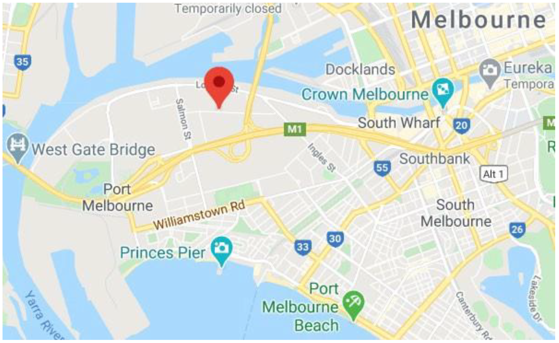
Given the significance of pavements as critical transport infrastructure, the research proposed a novel method to digitise the structure and monitor it through autonomous means. Recent advances in reality modelling, the development of digital twins, as well the growing paradigm of machine learning implementations in the construction industry suggested the possibility of an all-inclusive approach. The research selected a well-transited road (Turner Street) to be the subject of UAV flights, reality model creation, ML incorporation, and development of a cognitive digital twin. The cognitive digital twin has the capability to accurately depict the pavement in its current condition. Furthermore, it has the ability to detect current pavement distress such as cracking and rutting. The distress is in turn rated and provides a marker to the asset owner of potential maintenance strategies. The novelty of this approach is the use of UAV-obtained information in the shape of images and geospatial data. Road pavement reality models are developed, and ML is implemented to automate the detection of features. Turner Street, located in Port Melbourne, Victoria, has a length of approximately 1.2 km (see Figure 1). It is located in a reasonably transited industrial area, meaning a significant number of heavy vehicles make use of it on a daily basis.
Anecdotally, this road historically suffers continuous damage and has recently undergone surface maintenance. A significant issue is the ongoing maintenance. The ongoing costs associated with repairing the road cannot be easily justified for a relatively short section of road such as this. Given this, the pavement is left untreated for a significant period of time affecting local vehicles which could lead to a safety concern. These conditions make it a prime test bed to develop the continuous UAV surveillance proof of concept. The study demonstrated how the use of UAV continuous surveillance, the creation of a reality model, and eventually, a digital twin and the incorporation of ML can provide a cost-effective and enhanced monitoring of pavement structures.
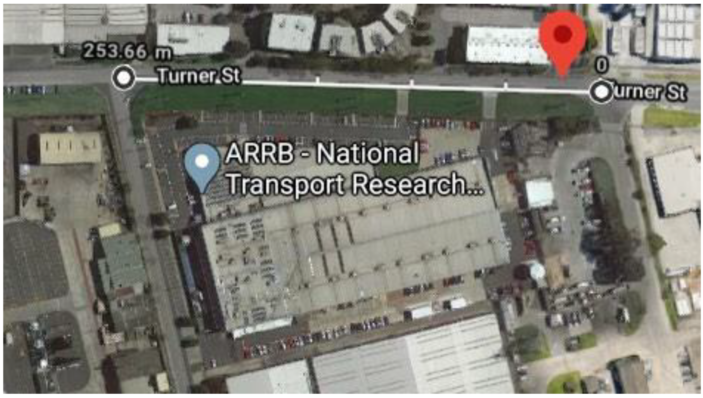
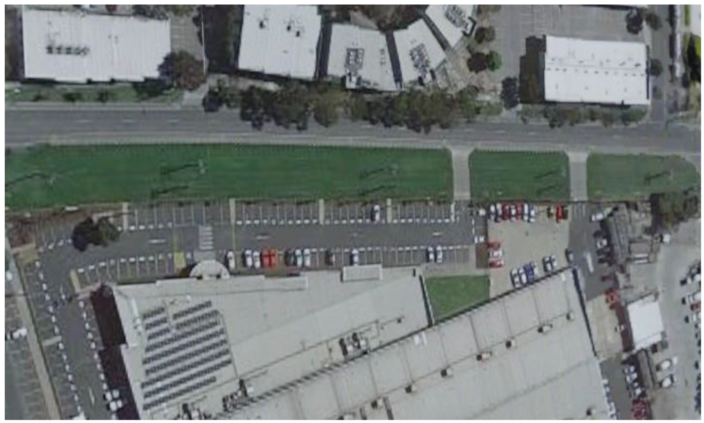
In this research, a series of different UAV flight methods were captured to develop the reality model. The equipment used for this study consisted of two Phantom 4 RTK (real time kinematics) drones with a D-RTK 2 base station. The embedded RTK system allows the drone to compare its World Geodetic System (WGS) coordinates with those recorded by survey points from the local council. This in turn allowed for more accurate measurements when recreating the pavement as a reality model. Figure 2 depicts the study area, which consisted of 250 m of road an initial reality model created with Google Maps; #D data can be seen in Figure 3. This was conducted to evaluate the potential outputs of the drone capture.
The captured footage allows for the creation of the cognitive digital twin once a reality model is developed alongside the ML algorithm to detect and score road distress.
Finally, the developed model was benchmarked against the current industry best practice on how to report pavement wear and current condition. At the moment, the most common (traditional) approach involves a team of technicians who drive alongside the road measuring and preparing a road quality assessment and condition monitoring report. The more sophisticated method involves a specialised vehicle, the advanced vehicle method, which continuously takes images of roads and laser data as it travels. The data collected are then sent to a third-party consultant who in turn analyses them through a custom algorithm that highlights road damage detection. By conducting a comparison to the current industry best practice, the proof of concept would be used to determine the effectiveness of the cognitive digital twin as an appropriate alternative. The research’s overarching goal was to identify this process as a cost- and time-efficient method when compared to current practices.
3. Data Acquisition
When acquiring the photographic data of the road, four different approaches were tested to ascertain the optimal method for the research. The UAV has the capability of capturing video and still images as well as flying along a predesignated flight path or manual flight control. All the four alternatives presented their own advantages and disadvantages in regard to data capture. The flight control method enables the user to input a predetermined flight path along a designated area. By doing so, the UAV can take images or video without the direct influence of the handler. However, this method presents two significant disadvantages. One is that the designated flight path for an area is predetermined by the on-board software of the UAV. To capture a square area means that a long rectangular object of interest (e.g., pavement) needs to be captured, meaning that a larger area than the one required will be flown over. This increases the time on air as well as the amount of unnecessary data and storage required. Furthermore, another disadvantage is that under a predetermined flight path, a minimum safe altitude is predisposed. For the study area, this was 100 m above ground. At this height, the detail on the defects of the road decreased. In summary, while a predetermined flight plan can be a suitable alternative, more time and storage need to be allocated and the height at which the images or video are captured needs to be accounted for. In contrast, a manual flight of the UAV yielded a faster capture time when compared to the predetermined flight. The 250 m of pavement was captured on video, and the total time taken was 3.24 min, while the programmed video plan was more than 8 min. The quality of the footage was significantly different. As previously mentioned, the predetermined flight method could capture footage at a height of 100 m, while the manual video method could capture data only at 60 m above ground. Both heights followed the appropriate regulations for the area of the study, yet the predetermined flight method considers the safest distance and cannot be overridden. Furthermore, the quantity of data captured was vastly different. The manual flight only captured the road features and nearby structures. However, the predetermined flight method captured surrounding buildings, which increased the post-processing time to recreate the road model as a reality model by 3 h. However, the better output was obtained from a manual flight while still images were taken. The manual flight with still images captured the 250 m in 10 min, which is three times longer than that of the video flight.
However, the data captured was more significant with less wastage of data. The manual still image activity required a more experienced UAV handler as they would be the ones judging when an image would need to be taken, and they would have to understand the required overlap for a photogrammetric model to be created. Nonetheless, the quantity of images/footage obtained drastically decreased when performing a manual still image flight. For instance, the manual video footage required a frame splicing at every 0.343 s to create a suitable reality model. This yielded 567 photographs to be analysed. In contrast, the still photo flight had only 205 photos. This difference meant a longer post-processing time was required to analyse the video data (7 h) when compared to the manual flight, which only required 2 h to create a reality model. In summary, for this research, the manual still image method was deemed the most suitable. However, the other three methods could be appropriate for other roads where a larger network needs to be captured or more data of the surroundings is needed.
4. Twin Development
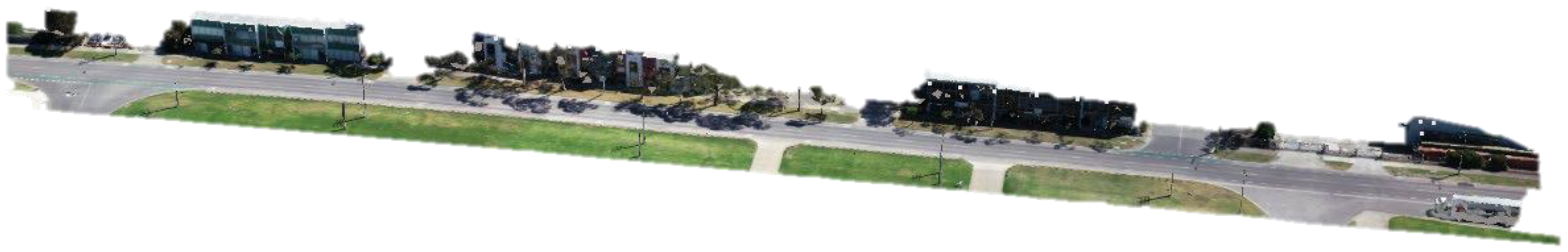
As mentioned in the previous section, data collected by the manual still photo method was selected as the most suitable to recreate the road. The data consisted of 205 images for 250 metres of road. When processing the images, the process took 2 h to yield a reality model. An image of the completed reality model can be seen in Figure 4.
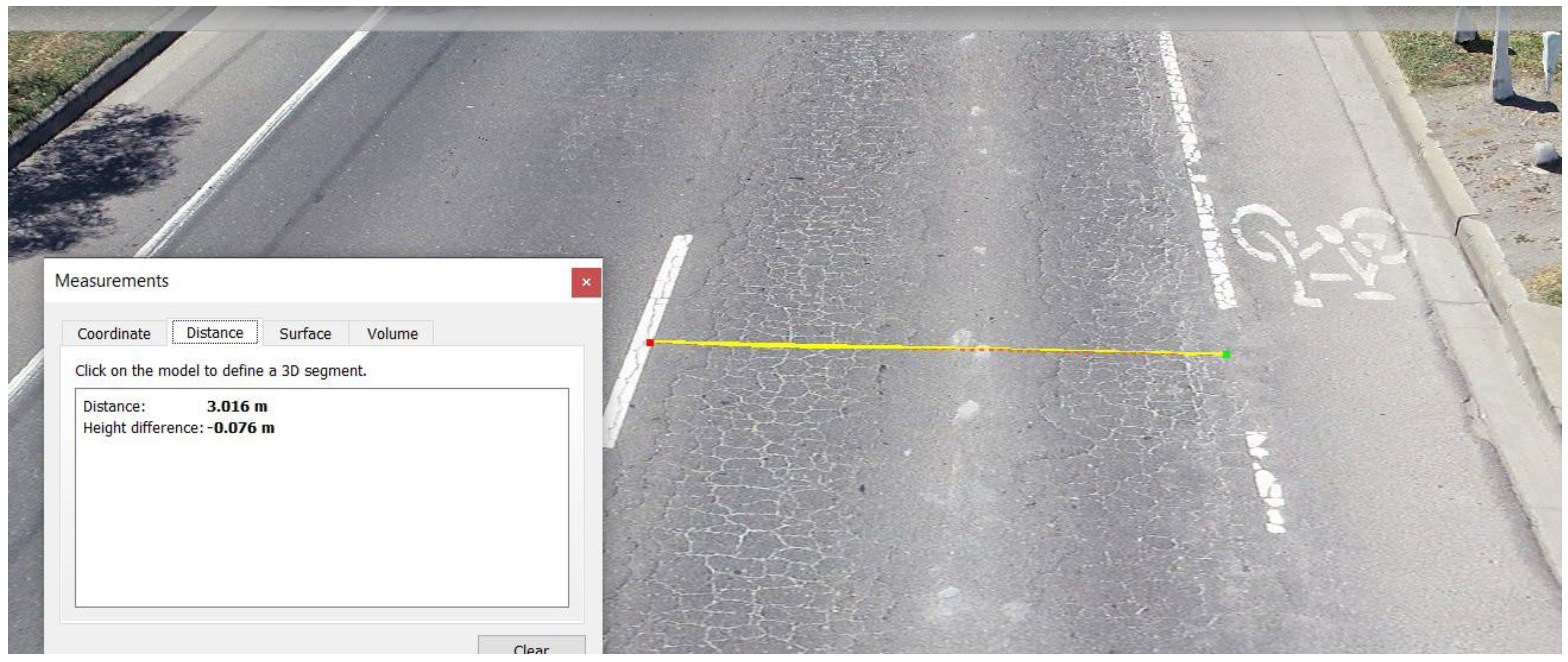
The results obtained from the reality model reflected an accurate representation of the current state of the road. This can be seen in Figure 5 where the distance from the bike path lane and the centre line measured 3.00 m ± 0.02 m across the entirety of the model with the corresponding slope.
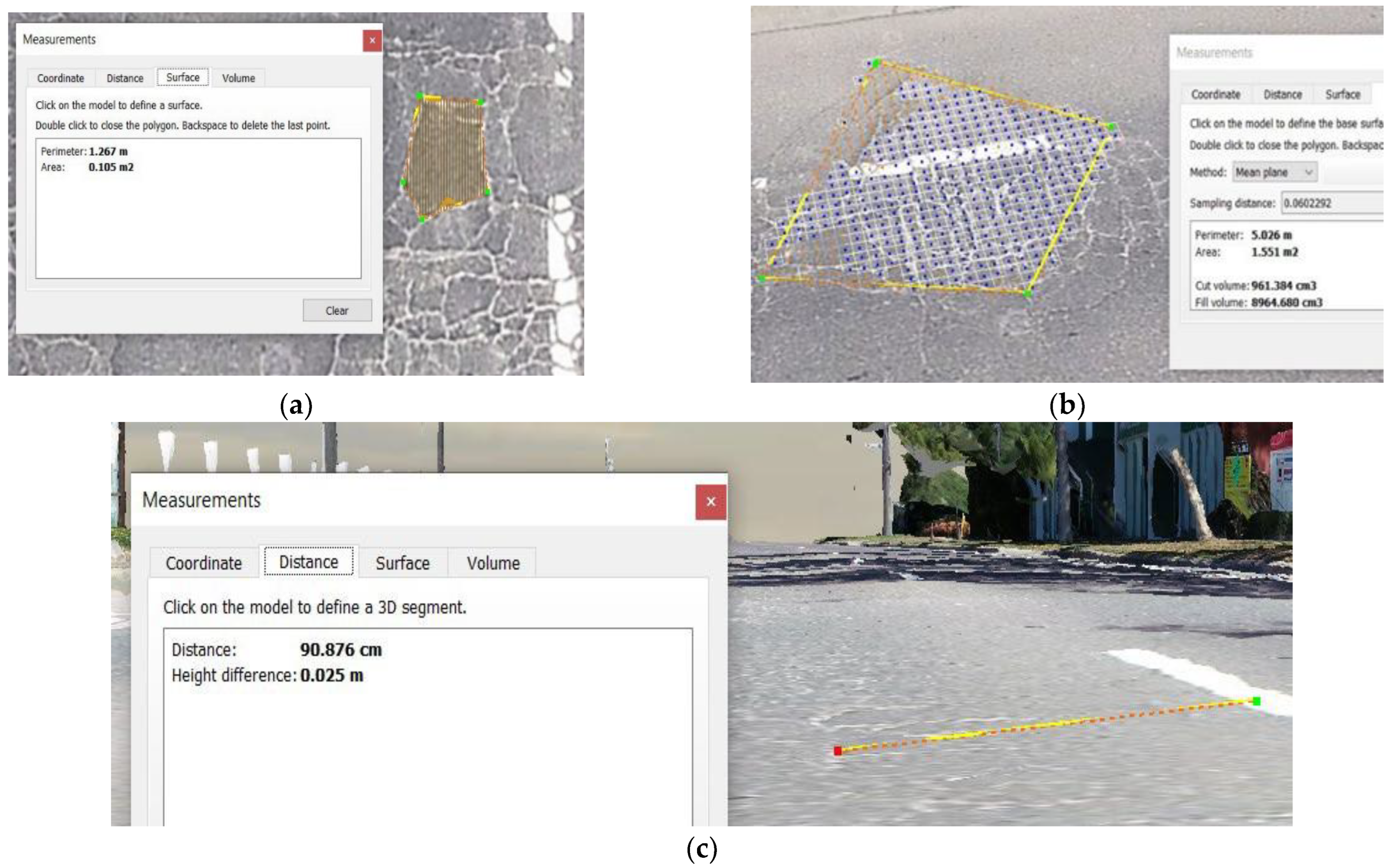
Furthermore, the model recreated a variety of defects in the road, including rutting, potholes, and crocodile cracking. The measurements seen in the reality model were accurate representations of the initial measurements taken from the defect in the road. These can be seen in Figure 6.
Given the success in the creation of an accurate reality model, the file was converted into a central dataset to incorporate information of the pavement structure.
5. Cognitive Twin Architecture
In this section, the details of image data processing, mask generation, architecture of the U-net, and the use of VGG16 as a feature extractor is discussed.
5.1. Network Architecture
5.1.1. U-Net Architecture
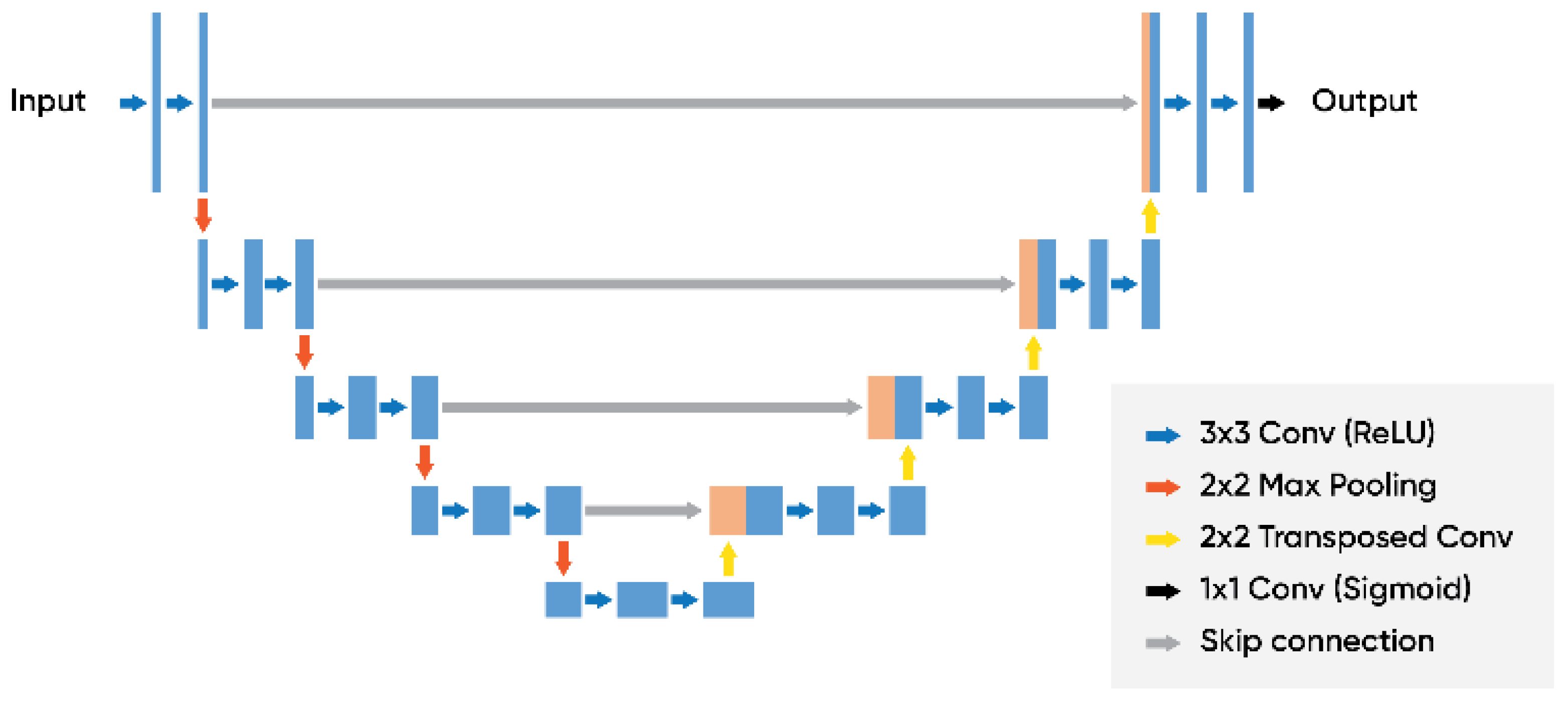
The U-Net network is commonly understood as a complete CNN network established in 2015 [45]. One of the unique features is that it does not need as many training sets as other CNN structures, as well as having an overall higher accuracy in terms of its segmentation. The U-Net architecture commonly has three distinct sections: (i) the contraction, (ii) the bottleneck, and (iii) the expansion sections. The first section, contraction, serves as the context gathering the information provided while also expanding the path to be used for a more precise positioning. This section is composed of multiple contraction blocks as depicted in Figure 7, where each block has an input of 3 × 3 applied to their convolution layer followed by a 2 × 2 maxpooling. Further, the feature map or kernel is present as double blocks in order for the architecture to accurately learn the complex features of the structure presented.
The layer at the bottom is responsible for mediating between the contracting and expanding layer. To do so, two 3 × 3 CNN layers followed by a 2 × 2 convolution layer are applied, shown in Figure 8. The number of characteristic channels is doubled by the activation function ReLu. However, at the core of the presented architecture is the expansion part. Not unlike the contraction layer, this section also consists of multiple expansion blocks. However, each block here goes through two inputs of 3 × 3 CNN layers with subsequent 2 × 2 unsampling layers. Furthermore, each of these blocks of feature maps is then used in the convolutional layer in order to maintain the desired symmetry. The input is appended frequently by the feature maps of the corresponding contraction layer. Furthermore, this action ensures that the features presented are fully learned while the image is being contracted and used in the reconstruction. In terms of how many expansion blocks are present, this matches that of the contraction block. Moreover, as the mapping is being produced, it undergoes another 3 × 3 CNN layer, where the number of feature maps is equal to that of the segments desired. The final layer consists of the expanding path, a 1 × 1 convolution kernel is applied to map each of the 2-bit eigenvectors of the output layer of the network. In this study, a road crack detection model was trained by a U-Net network with 23 convolution layers. The input image in this study had a resolution of 256 × 256 pixels. This network implements a sigmoid function as the activation function of the neurons as well as a cross- entropy for the cost function. It is noted that this increases the speed of weight updating, hence improving the overall training speed. On the other hand, a softmax function with a categorical cross-entropy was also trained and tested as a potential alternative.
5.1.2. Feature Extractor Using Transfer Learning
In order to avoid training a new model from scratch, transfer learning leverages the feature representations from a pre-trained model, where the models are trained on large datasets and serve as standard benchmark for the computer vision frontier. In fact, other computer vision tasks can also use the weights that are obtained from the models to directly make predictions on new tasks or help with new model training by becoming integrated. Particularly, for a small training dataset, transfer learning is quite convenient. For instance, in this study, the weights of the new model can be initialized by using the weights from the pre-trained models. One of the key benefits of pre-trained models is their usage in other real world applications due to their generic nature. An example would be the models that are trained on and used for real-world image classification problems. The reason for this is that these datasets can contain more than 1000 classes. So, these models can be used and fine-tuned in order to generate the desired features for the purpose of different machine learning models. In order to achieve that, firstly, the pre-trained model required for the studied problem needs to be attained. Then the base model needs to be created. For that, the base model needs to be initiated using one of the architectures such as VGG16. Additionally, the pre-trained weights can optionally be downloaded. In case the weights are not downloaded, then the architecture will need to be used to train the re-initialized set. Here, the learned knowledge that has already taken place will be lost unless they are not frozen. In fact, this would not be different from actually training the model from scratch. In such instances, the principle is to feed output of the convolution layer as input to a new model. In this way, the images can be pre-processed, and the essential features can be extracted by using the pre-trained model, or a part of it.
5.1.3. Loss Functions
When a deep learning algorithm is being trained and optimized, it is understood that there will be an error function referred to as a loss function. Among the loss functions, cross entropy is one of the most useful methods to better register unlikely events occurring [46]. The cross-entropy loss is defined in Equation (1), where C is the activation function, and is the activation functions.
Equations (2) and (3) refer to the binary cross entropy.
In Equation (4), X and Y are the two sets. Here it is used to calculate the Jaccard distance between the pavement images and the binary masks, given the continuous conductivity of loss function and to minimize the loss of the network. In this work, the network is trained to minimize the Jaccard distance from the Jaccard coefficient. The Jaccard index is also understood as the Intersection over Union (IoU), which is commonly employed when performing object detection. For the purpose of the research, it is critical to calculate the overlap ratio of the bounding boxes and the ground truth of the images. When handling pavement crack image segmentation, the result of segmentation can be viewed as the output of pixel classification. The pixels of a crack are classified as one; at the same time, the pixels of normal pavement condition are classified as zero. Therefore, in the presented model, the Jaccard Index is equal to the ratio of pixels where they are both classified as one in prediction and ground truth to the pixels which are classified as one in prediction or ground truth.
5.1.4. Parameter Optimization
Adam Optimizer
Adam is one of the most widely adopted algorithm optimizers in the deep learning field. First presented by Kingma and Lei Ba in 2015 [47], it presented itself as an efficient stochastic optimisation method. Unlike most common previous optimizers, Adam integrates an adaptive gradient algorithm and root mean square propagation. From its inception, multiple studies have been conducted to further optimize and apply the optimizer to various fields [48,49]. This includes the improvement of cognitive capabilities within the critical infrastructure space (e.g., pavements). Recent studies in machine learning apply a variety of CNNs with the Adam optimizer [50,51,52].
Activation Function
There are several types of activation functions when exploring the machine learning space. Two of the most commonly applied are sigmoid and softmax. Sigmoid, being a traditional approach, is used to give the probability of the output as it works in the range of zero to one. SoftMax also gives outputs from zero to one, but it has certain limitations as it calculates relative probabilities and needs sufficient learning data to function [53,54]. Both of these are seen in Equation (5) and Equation (6), respectively.
5.1.5. Performance Evaluation Matrices
One of the most widely adopted performance evaluations is that of the true/false positive and negative, where: (i) TP is true positive, (ii) TN is true negative, (iii) FP is false positive, and (iv) FN is false negative. The true aspect is understood to be when the predicted matches the actual result and false is when it does not. Precision is therefore understood as the percentage of the total positives/negatives that were captured. If it is equal to one, everything was predicted accurately, represented in Equation (7).
Recall and accuracy, shown in Equations (8) and (9), take into account the total actual results where once again if everything was accounted for it should be equal to one where FN is zero [55].
The F score is the overall function of the system. Intersection over Union refers to the ratio of the overlap and the union areas of the images being compared, shown in Equations (10) and (11).
5.2. Outcomes and Analysis
Dataset Preparation
In the initial stage, the noise is lessened with a median blur filter, since it is a well-known order statistic filter and has positive performance for instances where specific noise types such as “Gaussian,” “random,” and “salt and pepper” noises are found. In the median filter, it is found that the center pixel of an M × M neighborhood is replaced by adding the median value of a corresponding window. In these instances, noise pixels can be considered as being significantly different from that of the median. Using a median filter can remove these type of noise problems. The filter is used to remove the noise pixels on the pavement crack image before the binarization operation (e.g., thresholding). Both binary and Otsu thresholding is used. Binarization plays an important role in digital image processing, mainly in computer vision applications. Thresholding is an efficient technique in binarization. Binarization generally involves two steps, including the determination of a gray threshold according to some objective criteria and assigning each pixel to one class of background or foreground. If the intensity of the pixel is greater than the determined threshold, then it belongs to the foreground class and otherwise to the background. Binary thresholding is the most common and simplest type of thresholding, which results in creation of a binary image from a gray image, which is actually based on threshold values. Here we can specify the object target as either dark or light. Contrary to that, the Otsu’s thresholding method is different, as it rather corresponds to linear discriminant criteria, where it is assumed that the image consists of only the object (foreground) as well as the background. Additionally, the heterogeneity and diversity of the background are ignored in this case. The threshold is set by Otsu to try and minimize the overlap for the class distribution. By using Otsu’s method, the image is segmented into sets of two light regions as well as dark regions, T0 and T1. In fact, Otsu’s thresholding method can scan all types of possible sets of thresholding values. It also calculates the minimum value for the pixel levels that is available on each side of the threshold. Overall, the goal is to identify the threshold value while ensuring we get the minimum entropy for the sum of background and foreground. The optimal threshold value can be calculated by minimizing the sum of the weighted group variances, where the weights are suggested to be the probability of the respective groups. After extracting the background and foreground, the image is applied to the Canny Edge filters to detect the edges of that corresponding image, where a wide range of edges in the crack images are detected. It uses a filter, which is based on the derivative of a Gaussian, and it is conducted in this way to compute value of intensity for the gradients. Due to the use of the Gaussian, the effect of noise present in the image is reduced because the image retrieved from the thresholding method is further removed. As it is known, the road crack image noise properties are more critical than other image properties. Therefore, it is ensured that potential edges must be thinned down to low values (1-pixel curves and it is achieved by removing non-maximum pixels of the gradient magnitude. At the end, hysteresis thresholding on the gradient magnitude is used to determine whether edge pixels are kept or removed.
The general criteria for edge detection include:
- Detection of edges with low error rate, signifies that detection should catch as many edges shown in the image as possible with accuracy.
- The edge point detected by the operator should be accurately localized at the center of the edge.
- A given edge in the image should possibly be marked only once, and where appropriate, false edges should not be created by the image noise.
Morphological operations to shapes and structures inside of images are applied. As mentioned, the structuring element suggests the neighborhood to be examined around each of the pixels. In addition, various kinds of morphological operations already exist (e.g., dilation, opening, closing, erosion, morphological gradient, black hat). Therefore, based on the given operation and the size of the structuring element, the output image can be adjusted. At first, closing needs to be applied to fill in the lines where the closing is a dilation followed by an erosion. A closure is used to close holes inside objects or to connect components together. After that, an opening is applied to get rid of the noise (as the pavement crack image is highly biased due to noise). In this case, an opening is an erosion followed by a dilation method. Performing an opening operation allows us to remove small blobs from a particular image. At first, the small blobs are removed by applying the erosion, then a dilation is applied to ensure it regrows the size of an original object. After applying all the filters as discussed above, the mask for the training of the neural network can be developed.
5.3. CNN (VGG16) as a Feature Extractor
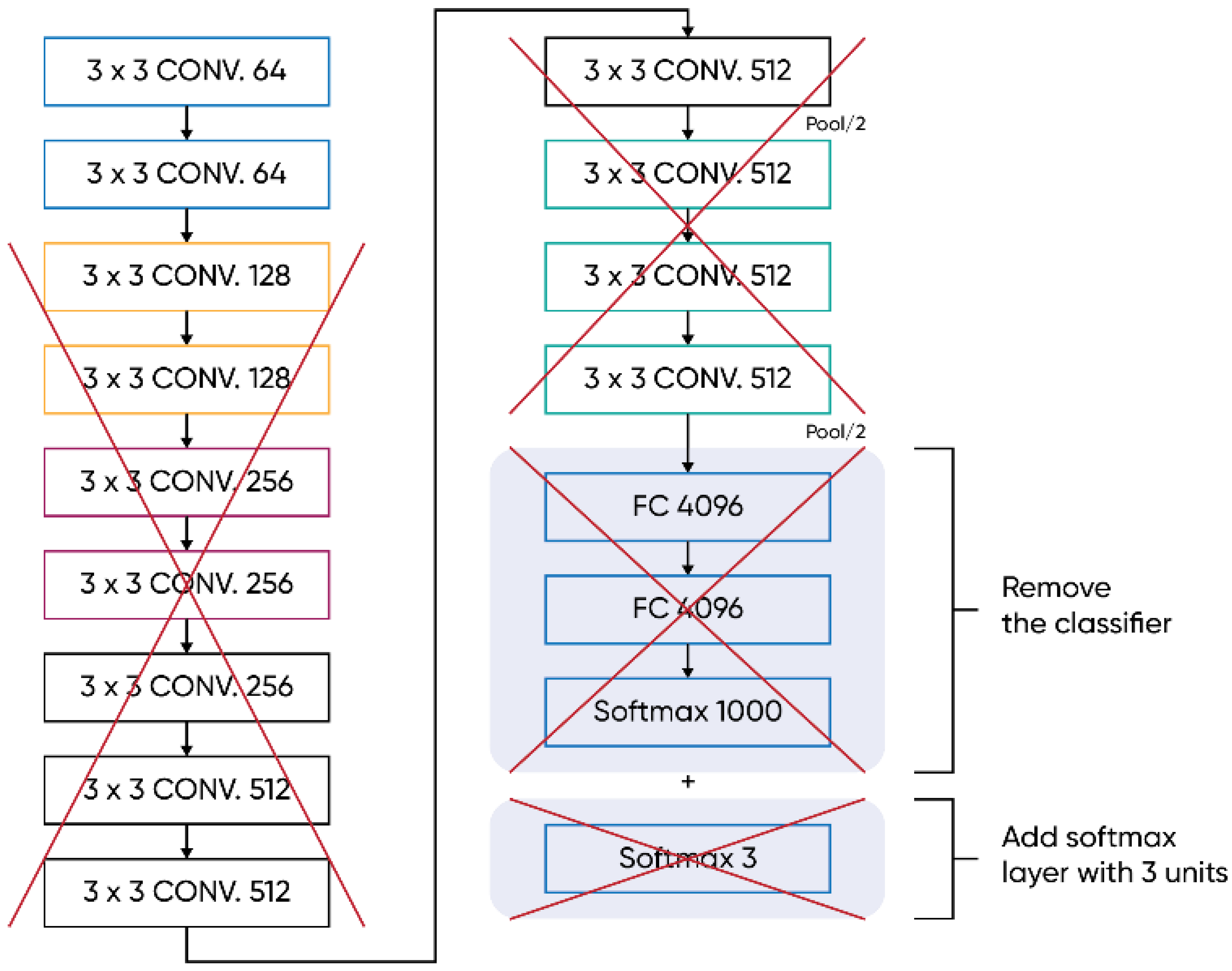
The application of transfer learning technology provides a state-of-the-art method for feature extraction. As the well-known CNN models have strong feature extraction abilities, employing them as feature extractors provide significant time savings (no training process). Therefore, VGG16 CNN was adopted as the feature extractor for the ML-based classifier. Meanwhile, parametric studies are implemented to confirm the effect of the relevant parameters on the detection results. Finally, the influence of different feature layers on the detection results is revealed by feature visualization. Transfer learning technology is the reuse of a pre-trained model on a new problem. With transfer learning technology, the weights that CNN had learned for ‘Question A’ are transferred to a new ‘Question B’. Some well-known CNN models (e.g., Alexnet, Googlenet, VGG16) were trained on the ImageNet database, which was used in the ImageNet Large-Scale Visual Recognition Challenge (ILSVRC). These CNN models had strong feature extraction ability and could classify images into 1000 object categories. Therefore, we employed these excellent models as feature extractors for crack detection. The network included a series of processing layers (e.g., convolutional layer, pooling layer, fully connected layer). RGB (three channels) images were used as the input for all networks. The first two convolutional layers were adopted where the image dimension changes. Further, only the first two convolution layers were taken and created a new model to extract features. An image dataset included RGB crack images (256 × 256 pixels) of a pavement. Among them, 90% of the images were used for training and 10% for testing the performance of the ML-based classifier KNN.
5.4. Numerical Findings
Since each crack pattern is random in pavement images, the original images captured by the UAV were cropped into smaller images. The performances of the training models were compared after they were trained with image sizes of 256 × 256 only. For training purposes the U-Net-based neural network was trained with two loss functions named binary cross entropy and Jaccard index distance. Additionally, KNN, Random Forest, and XGBboost models were also used for training purposes. For the purpose of a fair comparison, the models were trained for 50 epochs for each image size. Table 1 shows the comparison between the two loss functions. Since in image segmentation, accuracy is not the only metric for model evaluation, the Jaccard index was also used as the evaluation metric.
The Jaccard index is also known as Intersection-Over- Union (IoU), which is one of the most commonly used performance evaluation metrics in semantic segmentation. The Jaccard Index represents the area of overlap between the predicted segmentation and the ground truth. Table 1 shows that the proposed U-Net model performs better in the binary cross entropy loss functions compared to the Jaccard coefficient-based loss function in terms of accuracy and mean IOU.
This study also considers the VGG16 based transfer learning feature extractor model that fits into the machine learning classifiers for the segmentation. Table 2 summarizes the results of this technique. Here, multiple classifiers including KNN, Random Forest, XGBboost, were adopted for semantic segmentation. Comparing Table 1 and Table 2, it can be concluded that the U-Net-based model outperforms the transfer learning technique for crack detection.
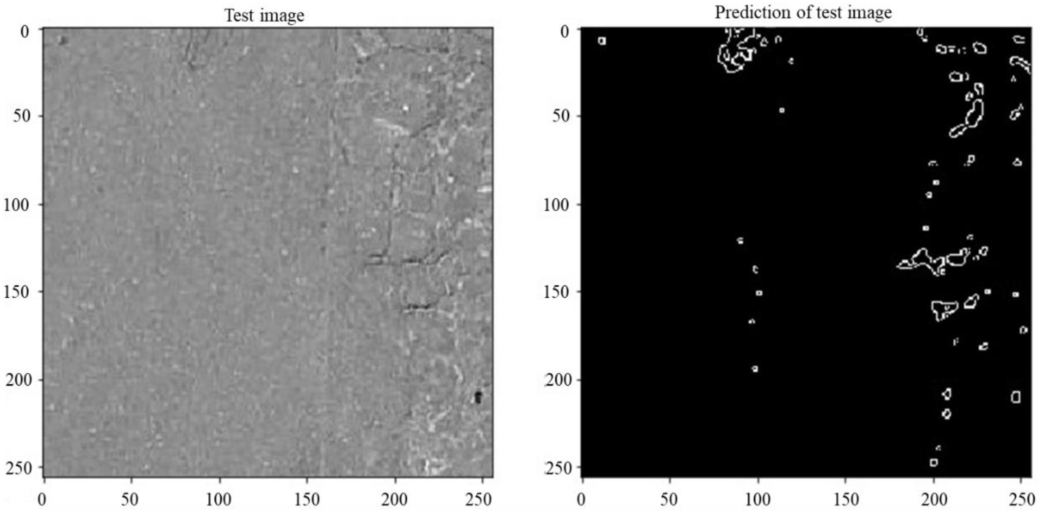
Figure 9 represents a prediction of cracks from a test image. The image in the left side of Figure 9 represents a testing image with cracks. The image in the right side shows the prediction on the test image. From the image, it can be suggested that the trained model successfully detects the cracks in the test image.
6. Cost Analysis
Given the successful creation of a pavement reality model and its export to be visualised in real time from any device at any time as a twin, as well as the ML defect detection developed, it is critical to consider its advantages against the more traditional methods. This included the traditional walking the road and the data captured from the advanced vehicle. A benchmarking was achieved by comparing the time and cost associated with producing a similar study/model. The cost and time comparison takes into account the equipment used by all three of the methods and the human labour involved in each. To perform a more accurate comparison, the cost and time to study 1 kilometre of road was considered as the benchmark all three would be compared against. The method presented here required the usage of a UAV, a Phantom 4 RTK drone with a D-RTK-2 base station, a computer with 16 GB of Ram and a graphics card, Nvidia GTX 1070, and the Bentley ContextCapture software package. The cost of the UAV equipment was estimated to be AUD 4000 and the computer to be AUD 3500. Both were considered to have a life of 5 years if used daily across the entire year. The cost per hour was AUD 0.13 and AUD 0.12, respectively. Similarly, the software package cost was AUD 1643.67 yearly, which yielded a total cost of AUD 0.26 per hour. For 1 km of road, the total time of flight of the UAV was estimated to be 0.67 hrs and 3 h of human labour, utilising both the software and the computer. For the purpose of this study, the cost of one skilled individual was considered to be AUD 65 per hour. This included all associated on-costs. Hence, the total time required to study one kilometre of road was 3.67 h at a cost of AUD 239.54. The complete breakdown can be seen in Table 3.
The traditional method of road condition monitoring involves two skilled individuals, one serving as the driver and the other as the report. In this process, a vehicle is used to traverse the road where the report will make notes, signal the driver where to stop, and take relevant measurements and images if required. Furthermore, this process covers approximately 10 kms of road every 4 h. A report is then produced by one of the individuals. This can take up to 3 h depending on the condition of the road and how many defects need to be highlighted. The cost breakdown assumed a cost for human labour of a highly trained individual of AUD 150 per hour and took the cost of the vehicle to be AUD 0.72 per km travelled as per the Australian Taxation Office. Given this, it was calculated that for 1 km of road to be studied, it would take 3.8 h and cost AUD 570.29. The breakdown of this can be seen in Table 4.
Furthermore, the final alternative is the use of an advanced vehicle. This method proved to be the costliest of the three. However, it produces detailed reports the other two do not. To produce a report on the road presented in its entirety (1.18 km), the quoted price was approximately AUD 6000 where one-third of the cost would be incurred in the creation of the report. It is understood that this value, on average, can be less if a larger road network is studied; however, for the purpose of this study, the aforementioned quote was considered. The advanced vehicle can travel at an average speed of 40–80 km/h. Hence, given the region of the road studied, 60 km/h was considered as the travel speed. The process would require a driver as well as a skilled technician to collect and process the data. Given the quote and the speed, it was concluded that it would take the advanced vehicle 0.03 h to travel 1 km and a total time of 2.1 h to complete the condition report at a total cost of AUD 5084.75. The breakdown can be seen in Table 5.
7. Discussion
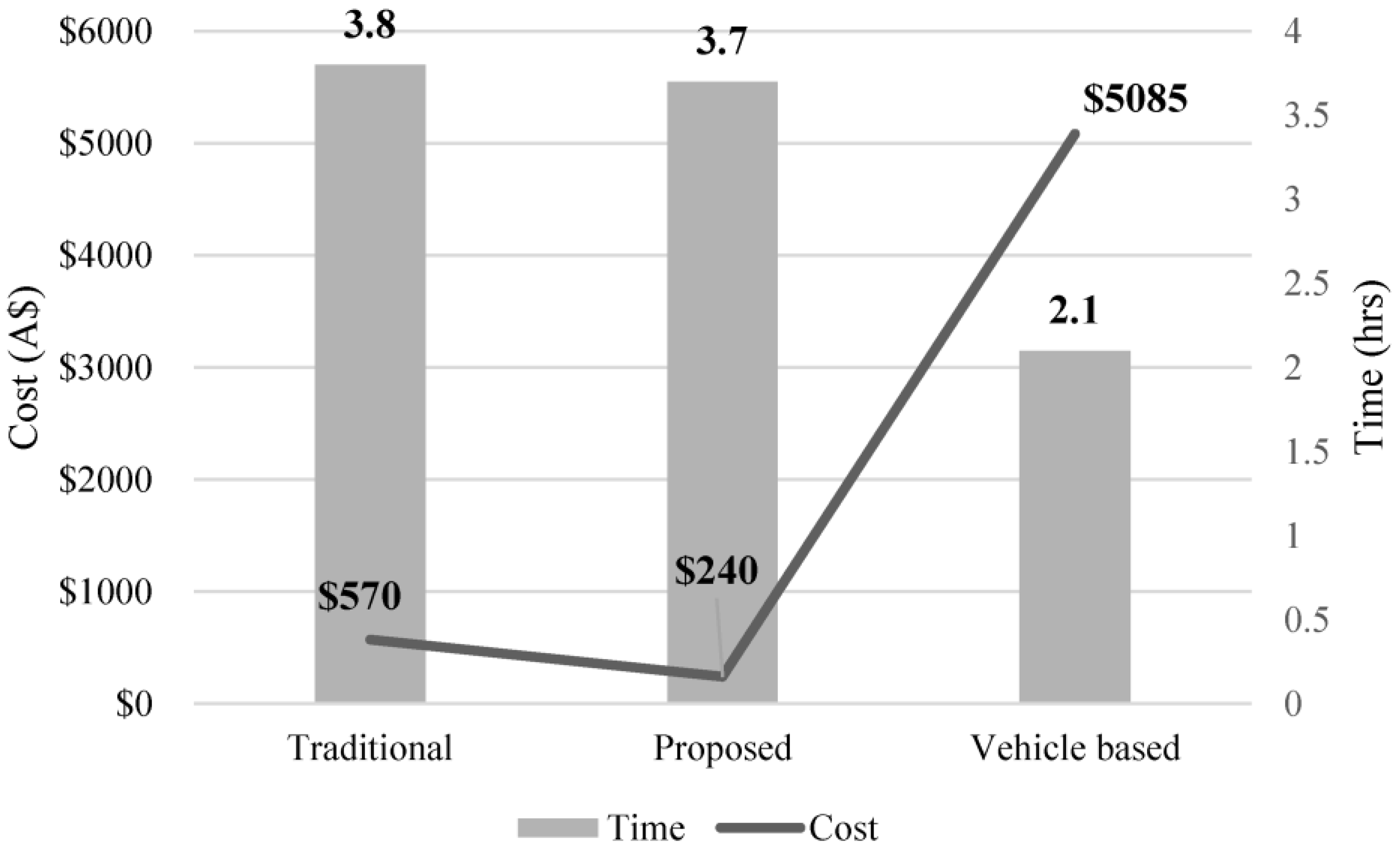
When comparing the three methods, there is a clear difference in cost between the traditional, the advanced vehicle, and the proposed method (automated method). The advanced vehicle costs almost 8 times more than the other two, as shown in Figure 10.
The reason behind this is the significant cost involved in using the advanced vehicle and producing its specialised road condition report. The report produced by the advanced vehicle outputs the highest quality reading of the three methods presented here, giving accurate readings of not only defects but current road roughness, among other conditions. However, this method would not be easily implemented across a series of networks as it often surpasses the budget of most road asset owners. Furthermore, there are only 14 such vehicles in existence worldwide, of which 2 reside in Australia, making it quite inaccessible to most asset owners (e.g., local councils).
Moreover, when comparing the proposed method to the traditional approach, it is evident that the new method is more cost effective per kilometer of road traveled by AUD 330, which can be significant over a large road network. Furthermore, the new method only requires one person to be involved in the process, whereas the other two require a second person to function as a driver at some point. The outputs of the proposed method and the traditional method are comparable as they can both give accurate reports of the pavement condition. However, the proposed method yields a model that can be easily accessed from any point and reviewed at any time, whereas the traditional method produces a conventional report. In terms of time, all three methods take similar amounts of time, with the advanced vehicle method being the fastest at 2.1 h, as also seen in Figure 10. While the advanced vehicle method can produce a quicker outcome, this is eclipsed when the costs are compared. Furthermore, between the traditional and proposed method, the latter took less time at 3.67 h in contrast to 3.8 h. Therefore, the proposed method when compared to the traditional method was quicker and lower cost.
Furthermore, the proposed method has the cognitive capability to recognize pavement defects, a function that would require a person in the traditional method to account for. A series of different architectures were tested as shown on Table 1 and Table 3, where the U-Net architecture with binary cross-entropy yielded the highest accuracy of 0.85. This implied that the current automated system can reliably detect damage to the pavement structure with a failure rate of less than 20%, which is quite acceptable. Hence, this allows the twin to be capable of highlighting areas of interest within the pavement against a predetermined threshold and allows for a predictive maintenance strategy to take place.
Accordingly, there are several challenges that must be noted when undertaking the automated method. While the use of UAVs can be streamlined, one of the significant difficulties is the altitude at which the drone must fly. As per most regulations, the drone must fly at an altitude of 60–100 m, as discussed in earlier sections. Capturing data at this altitude can result in unclear images and hard to detect features for the ML algorithm to detect. Furthermore, if not conducted under the proper daylight conditions, both the processing of the ML architecture and the development of the reality model/twin will be hindered. Further work is required in addressing the limits of the images that can be used for the development of this automated method. Furthermore, in terms of the post-processing challenges, the proposed ML architecture can detect significant pavement defects with moderate accuracy However, more data need to be assessed in order to gauge the limits of the U-Net architecture with binary cross-entropy to detect defects.
8. Conclusions
A key outcome of the study was to develop a proof of concept of historical road data being recorded accurately through a cognitive twin. This was achieved through the proposed method for the post-construction phase of pavement life cycle. The model, in turn, has to be able to accurately highlight the deterioration of the pavement over time, and the proposed model can identify the physical wear through this process. This study nearly halved costs although time saving was marginal. Further, the quality improvements and the availability of a cognitive twin for operational years were other advantages from this method.
Author Contributions
Conceptualization, methodology, software, validation, formal analysis, investigation, data curation, writing—original draft preparation, visualization, C.S.;Writing—review and editing, C.S., S.P., A.R. and A.K.; Supervision, resources, funding acquisition, administration, A.K.; Hub (https://sparchub.org.au (accessed on 10 June 2021)) at Monash University and Swinburne University of Technology. All authors have read and agreed to the published version of the manuscript.
Funding
This research was funded by the Australian Research Council: IH18.08.1.
Institutional Review Board Statement
Not applicable.
Informed Consent Statement
Not applicable.
Acknowledgments
This research work is part of a research collaboration project IH180800010 sponsored by the SPARC Hub (https://sparchub.org.au (accessed on 10 June 2021)) at Monash University and Swinburne University of Technology. As well as industry sponsor EON Reality Pte Ltd. The authors would like to express their special thanks to ARRB who facilitated the case study. The authors gratefully acknowledge the financial and in- kind support from SPARC Hub and EON reality without whom this research would not be possible.
Conflicts of Interest
The authors declare no conflict of interest.
References
- Department of Infrastructure, Transport, Regional Development, Communications and the Arts. Key Australian Infrastructure Statistics 2018. Bureau of Infrastructure and Transport Research Economics. 2018. Available online: https://www.bitre.gov.au/sites/default/files/infrastructure-statistics-yearbook-2018.pdf (accessed on 19 July 2019).
- Department of Infrastructure, Transport, Regional Development, Communications and the Arts. Key Australian Infrastructure Statistics 2019. Bureau of Infrastructure and Transport Research Economics. 2019. Available online: https://www.bitre.gov.au/sites/default/files/infrastructure-statistics-yearbook-2019.pdf (accessed on 12 January 2020).
- Infrastructure Australia. Australian Infrastructure Audit Report; ACT: Canberra, Australia, 2015.
- Guide to pavement technology: Part 1: Introduction to pavement technology; Austroads: Sydney, Australia, 2018.
- Department of Infrastructure and Regional Development, Australia. Trends: Infrastructure and Transport to 2030; Department of Infrastructure and Regional Development: Canberra, Australia, 2014. Available online: https://www.infrastructure.gov.au/sites/default/files/migrated/infrastructure/publications/files/Trends_Infrastructure_and_Transport_to_2030.pdf (accessed on 17 August 2019).
- Department of Infrastructure and Regional Development, Australia. Trends: Transport and Australia’s development to 2040 and beyond; Department of Infrastructure and Regional Development: Canberra, Australia, 2016. Available online: https://www.infrastructure.gov.au/sites/default/files/migrated/infrastructure/publications/files/Trends_to_2040.pdf (accessed on 20 August 2019).
- Department of Transport Victoria. Vicroads supplement to the austroads guide to road design: Introduction to vicroads supplement. Melbourne, Australia. 2012. Available online: https://www.vicroads.vic.gov.au/-/media/files/technical-documents-new/supplements-to-the-austroads-guide-to-road-design/supplement-to-agrd-part-6b--roadside-environment.ashx (accessed on 13 September 2019).
- Maroondah City Council. Maroondah city council engineering development design guidelines. Maroondah, Australia. 2016. Available online: https://www.maroondah.vic.gov.au/Development/Engineering-Development-Design-Guidelines (accessed on 22 August 2019).
- VicRoads Code of Practice RC 500.22—Selection and Design of Pavements and Surfacings; Department of Transport: Melbourne, Australia, 2018.
- Latrobe city, Latrobe city design guidelines. Latrobe, Australia. 2014. Available online: https://www.latrobe.vic.gov.au/sites/default/files/2021-04/FINAL%20FULL%20Latrobe%20Urban%20Design%20Guidelines%202021.pdf (accessed on 19 September 2019).
- De Carteret, R. Guide to Pavement Technology: Part 7: Pavement Maintenance; Austroads: Sydney, Australia, 2009. [Google Scholar]
- Jameson, G. Technical Basis of Austroads Guide to Pavement Technology Part 5: Pavement Evaluation and Treatment Design; Austroads: Sydney, Australia, 2021. [Google Scholar]
- Li, X.; Goldberg, D.W. Toward a mobile crowdsensing system for road surface assessment. Comput. Environ. Urban Syst. 2018, 69, 51–62. [Google Scholar]
- Souza, V.M.; Giusti, R.; Batista, A.J. Asfault: A low-cost system to evaluate pavement conditions in real-time using smartphones and machine learning. Pervasive Mob. Comput. 2018, 51, 121–137. [Google Scholar]
- RoadBotics. Available online: https://www.roadbotics.com/ (accessed on 29 November 2021).
- LeCun, Y.; Bottou, L.; Bengio, Y.; Haffner, P. Gradient-based learning applied to document recognition. Proc. IEEE 1998, 86, 2278–2324. [Google Scholar]
- Butcher, J.B.; Day, C.; Austin, J.; Haycock, P.; Verstraeten, D.; Schrauwen, B. Defect detection in reinforced concrete using random neural architectures. Comput.-Aided Civ. Infrastruct. Eng. 2014, 29, 191–207. [Google Scholar]
- Jiang, X.; Adeli, H. Pseudospectra, music, and dynamic wavelet neural network for damage detection of highrise buildings. Int. J. Numer. Methods Eng. 2007, 71, 606–629. [Google Scholar]
- Liu, S.-W.; Huang, J.H.; Sung, J.-C.; Lee, C. Detection of cracks using neural networks and computational mechanics. Comput. Methods Appl. Mech. Eng. 2002, 191, 2831–2845. [Google Scholar]
- O’Byrne, M.; Ghosh, B.; Schoefs, F.; Pakrashi, V. Regionally enhanced multiphase segmentation technique for damaged surfaces. Comput.-Aided Civ. Infrastruct. Eng. 2014, 29, 644–658. [Google Scholar]
- Wu, L.; Mokhtari, S.; Nazef, A.; Nam, B.; Yun, H.-B. Improvement of crack-detection accuracy using a novel crack defragmentation technique in image-based road assessment. J. Comput. Civ. Eng. 2016, 30, 4014118. [Google Scholar]
- Ahmadlou, M.; Adeli, H. Enhanced probabilistic neural network with local decision circles: A robust classifier. Integr. Comput.-Aided Eng. 2010, 17, 197–210. [Google Scholar]
- Ciresan, D.C.; Meier, U.; Masci, J.; Gambardella, L.M.; Schmidhuber, J. Flexible, high performance convolutional neural networks for image classification. In Proceedings of the Twenty-Second International Joint Conference on Artificial Intelligence, Barcelona, Spain, 19–22 July 2011. [Google Scholar]
- Krizhevsky, A.; Sutskever, I.; Hinton, G.E. Imagenet classification with deep convolutional neural networks. Adv. Neural Inf. Process. Syst. 2012, 25, 1097–1105. [Google Scholar]
- Soukup, D.; Huber-Mörk, R. Convolutional neural networks for steel surface defect detection from photometric stereo images. In International Symposium on Visual Computing; Springer: Cham, Switzerland, 2014; pp. 668–677. [Google Scholar]
- Golparvar-Fard, M.; Peña-Mora, F.; Savarese, S. D4ar–a 4-dimensional augmented reality model for automating construction progress monitoring data collection, processing and communication. J. Inf. Technol. Constr. 2009, 14, 129–153. [Google Scholar]
- Pătrăucean, V.; Armeni, I.; Nahangi, M.; Yeung, J.; Brilakis, I.; Haas, C. State of research in automatic as-built modelling. Adv. Eng. Inform. 2015, 29, 162–171. [Google Scholar] [CrossRef]
- Golparvar-Fard, M.; Savarese, S.; Peña-Mora, F. Automated model-based recognition of progress using daily construction photographs and ifc-based 4D models. In Proceedings of the Construction Research Congress 2010: Innovation for Reshaping Construction Practice, Banff, AB, Canada, 8–10 May 2010; pp. 51–60. [Google Scholar]
- De Villiers, J. Real-time photogrammetric stitching of high-resolution video on cots hardware. In Proceedings of the IEEE 2009 International Symposium on Optomechatronic Technologies, Istanbul, Turkey, 21–23 September 2009; pp. 46–51. [Google Scholar]
- Bhatla, A.; Choe, S.Y.; Fierro, O.; Leite, F. Evaluation of accuracy of as-built 3d modeling from photos taken by handheld digital cameras. Autom. Constr. 2012, 28, 116–127. [Google Scholar] [CrossRef]
- Silva, J.R.; Santos, T.T.; Morimoto, C.H. Automatic camera control in virtual environments augmented using multiple sparse videos. Comput. Graph. 2011, 35, 412–421. [Google Scholar] [CrossRef]
- Yang, M.-D.; Chao, C.-F.; Huang, K.-S.; Lu, L.-Y.; Chen, Y.-P. Image-based 3D scene reconstruction and exploration in augmented reality. Autom. Constr. 2013, 33, 48–60. [Google Scholar]
- Lin, K.; Liu, S.; Cheong, L.-F.; Zeng, B. Seamless video stitching from hand-held camera inputs. Comput. Graph. Forum 2016, 35, 479–487. [Google Scholar] [CrossRef]
- Sattar, S.; Li, S.; Chapman, M. Road surface monitoring using smart-phone sensors: A review. Sensors 2018, 18, 3845. [Google Scholar] [CrossRef]
- Otto, A.; Agatz, N.; Campbell, J.; Golden, B.; Pesch, E. Optimization approaches for civil applications of unmanned aerial vehicles (uavs) or aerial drones: A survey. Networks 2018, 72, 411–458. [Google Scholar]
- Puppala, A.J.; Congress, S.S.; Bheemasetti, T.V.; Caballero, S.R. Visualization of civil infrastructure emphasizing geomaterial characterization and performance. J. Mater. Civ. Eng. 2018, 30, 4018236. [Google Scholar] [CrossRef]
- Agnisarman, S.; Lopes, S.; Madathil, K.C.; Piratla, K.; Gramopadhye, A. A survey of automation-enabled human-in-the-loop systems for infrastructure visual inspection. Autom. Constr. 2019, 97, 52–76. [Google Scholar] [CrossRef]
- Zhang, C.; Elaksher, A. An unmanned aerial vehicle-based imaging system for 3D measurement of unpaved road surface distresses 1. Comput.-Aided Civ. Infrastruct. Eng. 2012, 27, 118–129. [Google Scholar] [CrossRef]
- Brooks, C.N.; Dean, D.B.; Dobson, R.J.; Roussi, C.; Carter, J.F.; VanderWoude, A.J.; Colling, T.; Banach, D.M. Identification of unpaved roads in a regional road network using remote sensing. Photogramm. Eng. Remote Sens. 2017, 83, 377–383. [Google Scholar] [CrossRef]
- Kubota, S.; Ho, C.; Nishi, K. Construction and usage of three-dimensional data for road structures using terrestrial laser scanning and uav with photogrammetry. In Proceedings of the ISARC International Symposium on Automation and Robotics in Construction; IAARC Publications: Oulu, Finland, 2019; Volume 36, pp. 136–143. [Google Scholar]
- Wang, R.; Peethambaran, J.; Chen, D. Lidar point clouds to 3-D urban models: A review. IEEE J. Sel. Top. Appl. Earth Obs. Remote Sens. 2018, 11, 606–627. [Google Scholar] [CrossRef]
- Xiong, X.; Adan, A.; Akinci, B.; Huber, D. Automatic creation of semantically rich 3D building models from laser scanner data. Autom. Constr. 2013, 31, 325–337. [Google Scholar] [CrossRef]
- Jaselskis, E.J.; Gao, Z.; Walters, R.C. Improving transportation projects using laser scanning. J. Constr. Eng. Manag. 2005, 131, 377–384. [Google Scholar] [CrossRef]
- Kim, P.; Chen, J.; Cho, Y.K. Slam-driven robotic mapping and registration of 3D point clouds. Autom. Constr. 2018, 89, 38–48. [Google Scholar] [CrossRef]
- Ronneberger, O.; Fischer, P.; Brox, T. U-net: Convolutional networks for biomedical image segmentation. In Medical Image Computing and Computer-Assisted Intervention—MICCAI 2015; Navab, N., Hornegger, J., Wells, W.M., Frangi, A.F., Eds.; Springer International Publishing: Cham, Switzerland, 2015; pp. 234–241. [Google Scholar]
- Murphy, K.P. Machine Learning: A Probabilistic Perspective; MIT Press: Cambridge, MA, USA, 2012. [Google Scholar]
- Kingma, D.P.; Ba, J. Adam: A method for stochastic optimization. arXiv 2014, arXiv:1412.6980. [Google Scholar]
- Bock, S.; Goppold, J.; Weiß, M. An improvement of the convergence proof of the adam-optimizer. arXiv 2018, arXiv:1804.10587. [Google Scholar]
- Khaire, U.M.; Dhanalakshmi, R. High-dimensional microarray dataset classification using an improved adam optimizer (iadam). J. Ambient Intell. Humaniz. Comput. 2020, 11, 5187–5204. [Google Scholar] [CrossRef]
- Gopalakrishnan, K. Deep learning in data-driven pavement image analysis and automated distress detection: A review. Data 2018, 3, 28. [Google Scholar] [CrossRef]
- Pei, L.; Sun, Z.; Xiao, L.; Li, W.; Sun, J.; Zhang, H. Virtual generation of pavement crack images based on improved deep convolutional generative adversarial network. Eng. Appl. Artif. Intell. 2021, 104, 104376. [Google Scholar] [CrossRef]
- Gopalakrishnan, K.; Khaitan, S.K.; Choudhary, A.; Agrawal, A. Deep convolutional neural networks with transfer learning for computer vision-based data-driven pavement distress detection. Constr. Build. Mater. 2017, 157, 322–330. [Google Scholar] [CrossRef]
- Sharma, S.; Sharma, S.; Athaiya, A. Activation functions in neural networks. Towards Data Sci. 2017, 6, 310–316. [Google Scholar] [CrossRef]
- Marreiros, A.C.; Daunizeau, J.; Kiebel, S.J.; Friston, K.J. Population dynamics: Variance and the sigmoid activation function. Neuroimage 2008, 42, 147–157. [Google Scholar] [CrossRef]
- Rottmann, M.; Maag, K.; Chan, R.; Hüger, F.; Schlicht, P.; Gottschalk, H. Detection of false positive and false negative samples in semantic segmentation. In Proceedings of the IEEE 2020 Design, Automation & Test in Europe Conference & Exhibition (DATE), Grenoble, France, 9–13 March 2020; pp. 1351–1356. [Google Scholar]
Figure 1.
Turner street map, Source: (htttps://www.google.com/maps (accessed on 18 October 2020)).
Figure 1.
Turner street map, Source: (htttps://www.google.com/maps (accessed on 18 October 2020)).

Figure 2.
Turner Street drone capture area, Source (https://www.google.com/maps (accessed on 26 October 2020)).
Figure 2.
Turner Street drone capture area, Source (https://www.google.com/maps (accessed on 26 October 2020)).

Figure 3.
Turner Street reality model.

Figure 4.
Turner Street reality model developed through photogrammetry.

Figure 5.
Measurement of bike path to centre line.

Figure 6.
Defects from the reality model: (a) crocodile cracking; (b) pothole; and (c) rutting.

Figure 7.
U-Net architecture.

Figure 8.
General architecture of cloud empowered data centric system.

Figure 9.
Predicting the cracks from the trained model using a new image.

Figure 10.
Cost and time comparison for 1 km of pavement.


Table 1.
U-net model performance comparison for two loss functions.
| Model | Loss Function | Accuracy | Intersection over Union |
|---|---|---|---|
| U-Net | Binary cross-entropy | 0.85 | 27 |
| U-Net | Jaccard coefficient | 0.51 | 19 |
Table 2.
VGG16-based transfer learning feature extractor.
| Model | Parameters | Precision | Recall | Accuracy | F-Score |
|---|---|---|---|---|---|
| K-nearest neighbour | n = 4 | 0.42 | 0.82 | 0.61 | 0.56 |
| n = 8 | 0.28 | 0.45 | 0.45 | 0.33 | |
| Random forest | N estimator = 100 | 0.29 | 0.47 | 0.47 | 0.32 |
| N estimator = 50 | 0.28 | 0.47 | 0.47 | 0.33 | |
| Extreme Gradient Boosting | - | 0.28 | 0.30 | 0.30 | 0.29 |
Table 3.
Cost breakdown.
| Equipment | Cost (AUD/h) | Time (h) | Subtotal Cost (AUD) |
|---|---|---|---|
| Unmanned aerial vehicle | 0.13 | 0.67 | 0.08 |
| Computer + software | 0.38 | 3.00 | 1.12 |
| Technician | 65.00 | 3.67 | 238.33 |
| Total cost | 239.53 |
Note: AUD 1 = 0.68 EUR.
Table 4.
Cost breakdown of traditional method.
| Equipment | Cost (AUD/h) | Time (h) | Subtotal Cost (AUD) |
|---|---|---|---|
| Vehicle consumption | 0.72 | 0.4 | 0.29 |
| Driver | 150.00 | 0.4 | 60.00 |
| Reporter | 150.00 | 3.4 | 510.00 |
| Total cost | 570.29 |
Table 5.
Cost breakdown of advanced vehicle method.
| Equipment | Cost (AUD/h) | Time (h) | Subtotal Cost (AUD) |
|---|---|---|---|
| Vehicle consumption | 0.72 | 0.03 | 0.03 |
| Advanced vehicle | 3386.14 | 1.00 | 3386.14 |
| Report software | 1394.92 | 1.00 | 1394.92 |
| Driver | 150.00 | 0.03 | 5.00 |
| Technician | 150.00 | 2.00 | 300.00 |
| Total cost | 5084.75 |
Publisher’s Note: MDPI stays neutral with regard to jurisdictional claims in published maps and institutional affiliations. |
© 2022 by the authors. Licensee MDPI, Basel, Switzerland. This article is an open access article distributed under the terms and conditions of the Creative Commons Attribution (CC BY) license (https://creativecommons.org/licenses/by/4.0/).
Share and Cite
MDPI and ACS Style
Sierra, C.; Paul, S.; Rahman, A.; Kulkarni, A. Development of a Cognitive Digital Twin for Pavement Infrastructure Health Monitoring. Infrastructures 2022, 7, 113. https://doi.org/10.3390/infrastructures7090113
AMA Style
Sierra C, Paul S, Rahman A, Kulkarni A. Development of a Cognitive Digital Twin for Pavement Infrastructure Health Monitoring. Infrastructures. 2022; 7(9):113. https://doi.org/10.3390/infrastructures7090113
Chicago/Turabian StyleSierra, Cristobal, Shuva Paul, Akhlaqur Rahman, and Ambarish Kulkarni. 2022. "Development of a Cognitive Digital Twin for Pavement Infrastructure Health Monitoring" Infrastructures 7, no. 9: 113. https://doi.org/10.3390/infrastructures7090113