Performance Evaluation of Blind Modal Identification in Large-Scale Civil Infrastructure

Abstract

The monitoring and maintenance of existing civil infrastructure has recently received worldwide attention. Several structural health monitoring methods have been developed, including time-, frequency-, and time–frequency domain methods of modal identification and damage detection to estimate the structural and modal parameters of large-scale structures. However, there are several implementation challenges of these modal identification methods, depending on the size of the structures, measurement noise, number of available sensors, and their operational loads. In this paper, two modal identification methods, Second-Order Blind Identification (SOBI) and Time-Varying Filtering Empirical Mode Decomposition (TVF-EMD), are evaluated and compared for large-scale structures including a footbridge and a wind turbine blade with a wide range of dynamic characteristics. The results show that TVF-EMD results in better accuracy in modal identification compared to SOBI for both structures. However, when the number of sensors is equal to or more than the number of target modes of the structure, SOBI results in better computational efficiencies compared to TVF-EMD.

1. Introduction

Large-scale civil infrastructures such as bridges and wind turbines are subjected to various external loads such as earthquakes, wind, traffic, and other environmental excitation during service life, resulting in rapid aging and structural deterioration [1,2]. In recent decades, Structural Health Monitoring (SHM) has attained significant interest to the infrastructure owners, structural engineers, and decision-makers as it provides powerful tools for the diagnosis and prognosis of as-is structural conditions [3]. Vibration-based modal identification methods utilize acceleration measurements to detect the physical and modal parameters that can be used for the identification and localization of damage [4,5]. However, there are several implementation challenges for these modal identification methods in different large-scale real-life structures such as bridges and wind turbines, depending on their overall dimensions, support conditions, measurement noise, number of available sensors, and operational loads [6,7]. This paper evaluates the performance of vibration-based SHM techniques in two full-scale structures subjected to these challenges.

Large-span bridges [8,9] and offshore wind turbines [10,11,12] caught worldwide attention recently. Bridges play a vital role in transportation infrastructure, which affects the economic growth and prosperity of a nation. A recent American infrastructure report card (2021) indicated that one-third of America’s infrastructure is at risk of significant deterioration, with about 240,000 bridges being at least 50 years old [13]. Similar to bridges, wind turbines are essential civil infrastructure for developing renewable wind energy, which has continuous resources with net-zero environmental impact [14,15]. However, the structural maintenance and rehabilitation of wind turbines are expensive; for example, the cost of repairing and constructing a blade varies between $30,000–200,000 USD [16]. Therefore, the SHM of wind turbines and bridges remains an essential consideration to various infrastructure owners, consulting firms, and government agencies worldwide. These condition-based health assessments enable them to develop a timely and optimum maintenance schedule, which is economical compared to replacing expensive structures [17].

Different failures can happen in blades, towers, and foundations of wind turbines. However, failure and damage to the blades are more common [18,19]. Due to limited accessibility and remote installation, very little research has been conducted to evaluate full-scale wind turbine systems [20]. Several numerical studies [21,22] and small-scale laboratory experiments [16,23] were conducted to diagnose wind turbines at both system and component levels. For instance, eight accelerometers were put on the tower of a wind turbine to assess its behavior during the construction and service life of the turbine [24]. Ou et al. (2021) monitored a laboratory-scale blade using accelerometers, temperature sensors, humidity sensors, and strain gauges under different operating conditions and external excitations.

Similar to wind turbines, the performance of bridges can be affected by external dynamic loads such as wind, earthquakes, and traffic loads. Moreover, environmental conditions, including temperature, humidity, and corrosive situations, can cause significant damage and cracks in different elements of bridges during their service life [25]. Bridge damage includes cracks in concrete elements, displacement and vibration that is more than the acceptable range, connections failure, welds failure, corrosion in foundations and piles, and even failure of elements such as piers. On the other hand, as bridges are more slender than other civil structures, they experience a higher range of vibration due to ambient and man-made excitations, making them more susceptible to damage [26]. A lot of research focused on vibration-based bridge health monitoring methods to assess the safety of these structures [27,28]. However, optimal sensor placement, limited availability of sensors, inaccessibility, and measurement noise pose several challenges in this field, which has caught significant attention in recent years [29,30]. This emphasizes the need for an increasing number of real-life validations of the infrastructure monitoring technology and damage detection techniques.

Structural damage results in changes in the modal properties of the structure, such as natural frequencies, damping ratios, and mode shapes [31,32]. Although modal identification techniques rely on measurements, such as strain, displacement and acceleration, monitoring and obtaining these measurements from full-scale structures still poses significant challenges [33]. Moreover, the measured data are often noisy, which affects the accuracy of modal identification [34]. There has been significant development of various modal identification methods that can resolve the SHM challenges of bridge and wind turbines using time-domain (TD), frequency-domain (FD), and time–frequency domain (TFD) methods [35]. The TD and FD techniques can be applied for stationary and linear signals; however, complex excitations are non-stationary in nature [36]. Hence, the TFD methods have been developed as a new field in SHM [37,38]. Moreover, TFD methods are more robust and faster than other TD methods, such as Stochastic Subspace Identification (SSI) [39]. For example, SSI requires model order selection and stabilization diagrams, which require significant user intervention [39].

There are several TFD methods, such as Wavelet Transform [40], Empirical Wavelet Transform, Hilbert Huang Transform [41], Empirical Mode Decomposition (EMD) [42,43], and Time-Varying Filtering Empirical Mode Decomposition (TVF-EMD) [44]. Unlike Wavelet Transform methods, EMD is one of the popular SHM techniques as it is free of any basis function and undertakes decomposition based on a local characteristic of the data of a single-channel measurement. Mixed multicomponent signals can be decomposed by the EMD method into Intrinsic Mode Functions (IMFs). TVF-EMD is one of the variants of EMD, which is free of mode-mixing [45]. Blind Source Separation (BSS) [46] and Second-Order Blind Identification (SOBI) [47,48], which are TD methods, can recover individual modal response components from the measurements. Unlike other modal identification methods such as SSI, SOBI or TVF-EMD does not require user-intensive steps, including stabilization diagrams and model order selection. Both SOBI and TVF-EMD methods have been used in the literature to assess laboratory-scale models of buildings, bridges, and a few small-scale full-scale structures [47,49]. However, more studies are necessary for the identification of closely-spaced frequencies of a wide range of large structures. Therefore, in this paper, both of these output-only modal identification methods (i.e., TVF-EMD and SOBI) have been implemented into two full-scale structures, including a bridge and wind turbine, with a broad range of frequency characteristics.

There are several technical challenges to monitoring full-scale structures, which makes the procedure expensive and time-consuming. Due to accessibility issues and harsh environments, the physical instrumentation of these structures remains unsafe and costly. For example, monitoring wind turbines needs reliable wireless sensors for freezing temperatures and special data acquisition systems [19,33]. Some non-destructive techniques, such as infrared thermography, were introduced for SHM to overcome accessing problems [50]. However, these methods are not reliable for monitoring all structures, especially in harsh environments, as they are dependent on environmental conditions such as low temperatures [19]. On the other hand, to monitor full-scale structures requires using numerous and various equipment for a long period of time to obtain comprehensive data. For example, Queensferry bridge was monitored using nearly 2000 different types of sensors for 3 years [51]. Moreover, five long-span, cable-supported bridges in Hong Kong, including Tsing Ma, Kap Shui Mun, Ting Kau, Western Corridor, and Stonecutters, were monitored by ~1700 sensors for each bridge. Therefore, another challenge in monitoring these huge structures is designing a complicated SHM system, a detailed sensing network, and an instrumentation strategy to acquire and collect the required data continuously [33]. Hence, a lot of research has been undertaken on the placement of sensors to optimize the measurement and monitoring strategy to estimate the valuable and critical dynamic properties of the structures [6,29].

The development of monitoring systems and sensors causes an tremendous increase in measuring data [19]. Although collecting more and more data is beneficial for comprehensive condition-based health assessments and confident decision-making, it results in the “big data” problem in SHM. The big data problem can be defined by three aspects, including volume, velocity, and variety. Regarding the volume characteristic, the most significant technical challenges remain the collection, transmission, and analysis of the data. Therefore, a new field of research regarding the value of information and information analysis in Civil Engineering has been developed. These studies aim to develop approaches for reliable and low-cost sensor placement and health monitoring of the structures [52,53,54]. In addition, the big data problem refers to the complexity (velocity and variety aspects) of datasets, which needs a new generation of data-processing equipment for coding, analyzing, visualizing, and filtering the data. Moreover, a considerable level of noise inevitably will exist in field measurements due to environmental conditions that affect the accuracy of SHM. Hence, high-accuracy filtering systems and equipment with a low-level of error are necessary [19]. Several researchers focus more on noise effects and lots of filters to minimize the effects of noise [55,56].

There are limited full-scale studies to demonstrate the performance of TVF-EMD and SOBI and compare their relative merits in real-life applications. Considering the abovementioned challenges of blind modal identification, this paper explores two full-scale structures, including a footbridge [57] and a wind turbine blade [58], as two valuable case studies to validate and compare the accuracy of a TD and TFD method. Therefore, this paper results in a better understanding of the performance and accuracy of these modal identification methods using two full-scale case studies. The paper is organized as follows. The modal identification methods are discussed in Section 2, and the case study structures are explained in Section 3. The results of the structural condition assessments are presented in Section 4, followed by key conclusions in Section 5.

2. Modal Identification Methods

In this paper, two different modal identification techniques, including SOBI (i.e., a TD method) and TVF-EMD (i.e., a TFD method), are evaluated and compared. The methodologies of these techniques are briefly described below.

2.1. Second-Order Blind Identification Method

Blind source separation estimates the hidden sources of a suite of multicomponent signals using their second-order or higher-order statistics. In particular, SOBI can analyze signals with different spectral contents by utilizing the temporal structure of the sources for a better separation of the signals [59]. This method is one of the most potent modal identification methods, even if the measurements are noisy. SOBI estimates the autocorrelation functions of both the sources and the noise in the subsequent stage. Hence, the calculation of noise variance before the extraction of source signals is not needed. Therefore, the accuracy of the method is independent of the noise distribution [48].

SOBI is advantageous over other system identification methods as it requires only output data to estimate modal parameters, which makes SOBI especially great for existing structures where input data may not be known. The SOBI formulation begins with the basic equation of motion [59]:

$$\left[M\right]\left\{\ddot{x}\left(t\right)\right\}+\left[C\right]\left\{\dot{x}\left(t\right)\right\}+\left[K\right]\left\{x\left(t\right)\right\}=\left\{F\left(t\right)\right\}$$

(1)

where $\left[M\right]$, $\left[C\right]$, $\left[K\right]$ is the mass, damping, and stiffness matrix; $\left\{x\left(t\right)\right\}$ is the displacement vector; and $\left\{F\left(t\right)\right\}$ is the force vector.

The solution to the equation of motion may be written as a summation of several vibration modes in matrix form:

$$\left\{x\left(n\right)\right\}=\left[A\right]\left\{s\left(n\right)\right\}$$

(2)

where $\left\{x\left(n\right)\right\}$ is the measurement matrix components of x, $\left[A\right]$ is the modal transformation matrix, and $\left\{s\left(n\right)\right\}$ is the matrix of the corresponding modal components.

To find $\left[A\right]$, two covariance matrices at time 0 and p are diagonalized [59]:

$$\left[R_x\left(0\right)\right]=E\left[\left\{x\left(n\right)\right\}{\left\{x\left(n\right)\right\}}^T\right]=\left[A\right]\left[R_s\left(0\right)\right]{\left[A\right]}^T$$

(3)

$$\left[R_x\left(p\right)\right]=E\left[\left\{x\left(n\right)\right\}{\left\{x\left(n-p\right)\right\}}^T\right]=\left[A\right]\left[R_s\left(p\right)\right]{\left[A\right]}^T$$

(4)

where $\left[R_s\left(p\right)\right]=E\left[\left\{s\left(n\right)\right\}{\left\{s\left(n-p\right)\right\}}^T\right]=\left[I\right]$. First, the responses are whitened, which removes any correlation two responses may have had:

$$\left[R_x\left(0\right)\right]=E\left[\left\{x\left(n\right)\right\}{\left\{x\left(n\right)\right\}}^T\right]=\left[V_x\right]\left[{\lambda }_x\right]{\left[V_x\right]}^T$$

(5)

where $\left[V_x\right]$ is the eigenvector matrix and $\left[{\lambda }_x\right]$ is the eigenvalue matrix. The whitened signals are computed using the following expression [60]:

$$\left\{\overline{x}\left(n\right)\right\}={\left[{\lambda }_x\right]}^{-1/2}{\left[V_x\right]}^T\left\{x\left(n\right)\right\}=\left[Q\right]\left\{x\left(n\right)\right\}$$

(6)

where $\left[Q\right]$ is the whitening matrix.

$$\left[R_{\overline{x}}\left(0\right)\right]=E\left[\left\{\overline{x}\left(n\right)\right\}{\left\{\overline{x}\left(n\right)\right\}}^T\right]=\left[I\right]$$

(7)

$\left[R_x\left(p\right)\right]$ becomes $\left[R_{\overline{x}\left(p\right)}\right]$ from the whitening process:

$$\left[R_{\overline{x}\left(p\right)}\right]=\frac{1}{N}\left[{{\displaystyle \sum }}_{n=1}^N\left\{\overline{x}\left(n\right)\right\}{\left\{\overline{x}\left(n-p\right)\right\}}^T\right]=\left[Q\right]\left[R_x\left(p\right)\right]{\left[Q\right]}^T=\left[Q\right]\left[A\right]\left[R_s\left(p\right)\right]{\left[A\right]}^T{\left[Q\right]}^T$$

(8)

$\left[R_{\overline{x}\left(p\right)}\right]$ is now diagonalized:

$$\left[V_{\overline{x}}\right]\left[R_{\overline{x}}\left(p\right)\right]{\left[V_{\overline{x}}\right]}^T=\left[{\lambda }_{\overline{x}}\right]$$

(9)

Since $\left[{\lambda }_{\overline{x}}\right]$ has distinct eigenvalues, the mixing matrix is estimated by:

$$\left[\widehat{A}\right]={\left[Q\right]}^{-1}\left[V_{\overline{x}}\right]=\left[V_x\right]{\left[{\lambda }_x\right]}^T\left[V_{\overline{x}}\right]$$

(10)

Finally, unitary transformation is performed to acquire the modal responses in the time domain:

$$\left\{\widehat{s}\left(n\right)\right\}={\left[\widehat{A}\right]}^{-1}\left\{x\left(n\right)\right\}$$

(11)

where $\left\{\widehat{s}\left(n\right)\right\}$ is the modal response.

2.2. Time-Varying Filtering Empirical Mode Decomposition Method

EMD is one of the data-driven TFD methods that does not need basic functions and can analyze non-linear and non-stationary signals [61]. EMD converts the measured data into a suite of mono-component signals called IMFs. IMFs are identified using a sifting process that employs a finite number of averaging and interpolation operations. However, the sifting process often results in a considerable mode mixing in the IMFs. Several adaptations of EMD were established to address this limitation of EMD. This problem has been solved by applying a Time-Varying Filtering (TVF) operation [44].

In the TVF-EMD method, a local cutoff filter is used to filter measurement data into local high-pass and low-pass elements to decompose into a suite of narrowband signals. In contrast to EMD, TVF-EMD does not require symmetric properties of upper and lower envelopes and intermittency criteria [61]. In fact, energy-based thresholding is often used to find out the energy concentration and eliminate the noise components to better delineate the modal responses. More details about such approaches can be found elsewhere [6]. B-spline approximation, which is based on developing polynomial splines with time-varying cutoff frequency, is used to define TVF. IMFs can be estimated in B-spline space, as shown below [44]

$$b_{ v}^p\left(t\right)={{\displaystyle \sum }}_{k=-\infty }^{+\infty }q\left(k\right){\beta }^p\left(\frac{t}{v}-k\right)$$

(12)

where q(k) is the B-spline coefficient, and it is expanded by v, which is the step size of the knot sequence and is used to combine the polynomial components. The q(k) is determined using the B-spline approximation that minimizes the error. Hence, for a measurement signal, x(t) and q(k) can be obtained by minimizing the error, as presented below:

$${\delta }_{ v}^2={{\displaystyle \sum }}_{t=-\infty }^{+\infty }{\left(X\left(t\right)-{\left\{q\right\}}_{\uparrow v}\ast W_v^p\left(t\right)\right)}^2$$

(13)

where ${\left\{-\right\}}_{\uparrow v}$ is the up-sampling function by v. $W_v^p\left(t\right)$ is considered equal to ${\beta }^p\left(t/v\right)$, and the asterisk shows the convolution operator. Therefore, $q\left(k\right)$ can be obtained as:

$$q\left(k\right)={\left\{c_v^p\ast x\right\}}_{\downarrow v}\left(k\right)$$

(14)

$$c_v^p={\left\{{\left({\left\{w_v^p\ast w_v^p\right\}}_{\downarrow v}\right)}^{-1}\right\}}_{\uparrow v}\ast w_v^p$$

(15)

$$b_v^p={\left\{c_v^p\ast x\right\}}_{\downarrow v}\ast w_v^p\left(t\right)$$

(16)

where ${\left\{-\right\}}_{\downarrow v}$ is the down-sampling function by v, and $c_v^p$ is the pre-filter discussed in Equation (15). The autocorrelation function of the modal response is then used to find the total damping ratio. Autocorrelation is performed using:

$$R_{ff}\left(\tau \right)={{\displaystyle \int }}_{-\infty }^{\infty }f\left(t\right)\overline{f\left(t-\tau \right)}dt$$

(17)

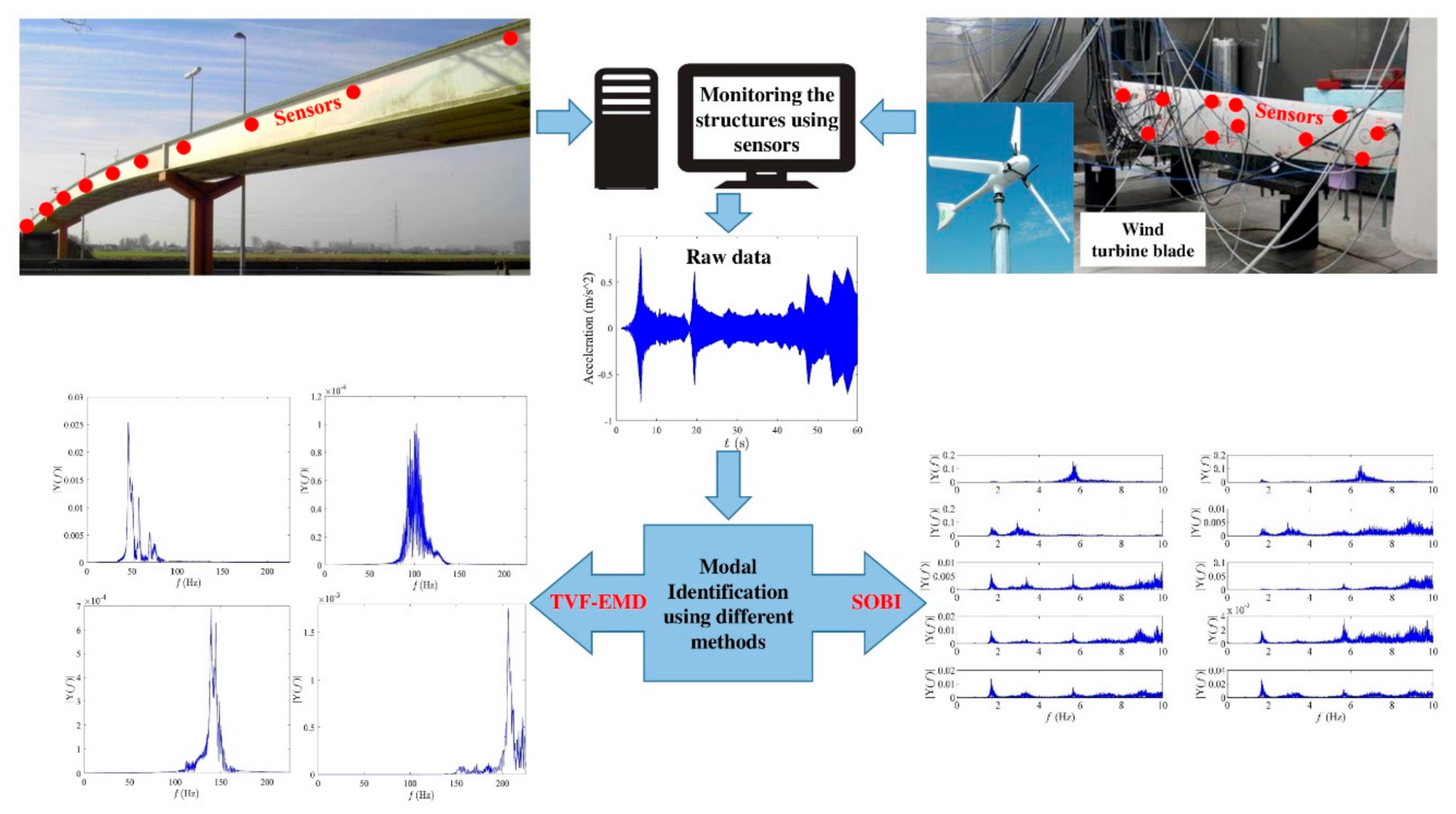
where $f\left(t\right)$ is the modal response, $\overline{f\left(t\right)}$ is the complex conjugate of $f\left(t\right)$, and τ is the time lag. The outline of the case studies employing two real-life examples using two modal identification methods is illustrated in Figure 1.

3. Case Studies

In this paper, two full-scale structures, including the Eeklo Pedestrian Bridge and a wind turbine, are studied. The details of these structures are discussed below.

3.1. Eeklo Pedestrian Bridge

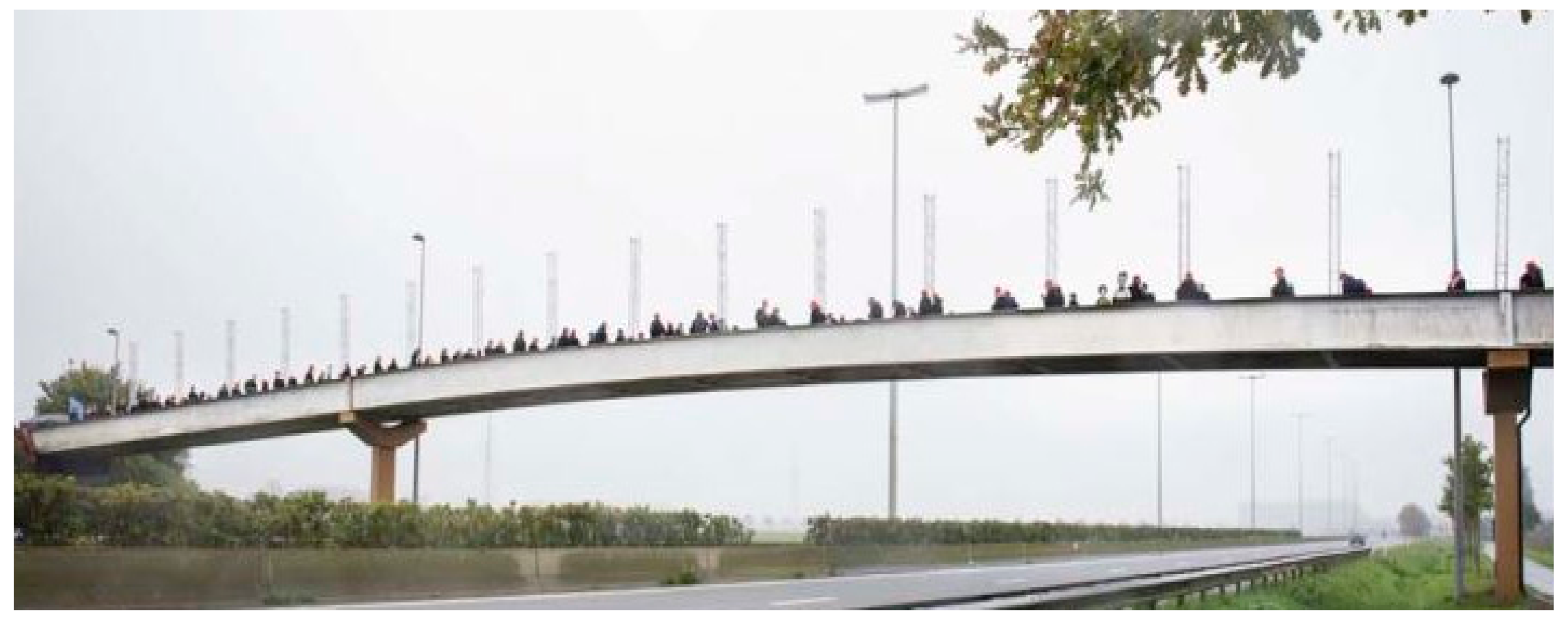
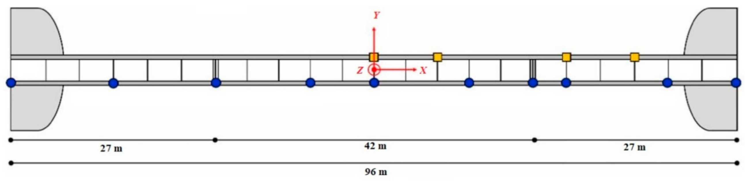
The Eeklo Bridge in Belgium was monitored in 2017 by Van Nimmen et al. (2021), as shown in Figure 2. They developed a finite element model of the bridge and compared the numerical and experimental study [57]. This bridge has a length of 96 m and consists of three spans (the middle span is 42 m and the two other spans are 27 m). Two main steel beams (1.2 m height), a steel deck (8 mm thickness), and three secondary steel beams were considered in the cross-section. The bridge was supported with two abutments at each end, and two piers along the bridge [62]. Twelve modes with frequencies up to 10 Hz and the corresponding modal damping ratios were identified [57]. Therefore, there is a wide range of frequencies for the validation of the SOBI and TVF-EMD methods, and for this reason, the Eeklo Bridge has been chosen as the ideal candidate for the case studies in this paper. The bridge was monitored under ambient- and pedestrian-induced excitations using 10 tri-axial accelerometers. The measurement grids and the coordinate system are shown in Figure 3. Ten different tests, including OMA (ambient excitation) and pedestrian excitation, were considered for the bridge testing. The summary of the test information is presented in

Table 1. Monitoring tests of the Eeklo Bridge [57].

Test #	Name	Duration (sec)	Description
A-A	OMA_A	900	OMA
A-1	W073_free-1	720	Free walking, 73 persons
A-2	W073_free-2	660	Free walking, 73 persons
A-3	W073_free-3	649	Free walking, 73 persons
A-4	W072_free-4	1860	Free walking, 72 persons
B-B	OMA_B	1200	OMA
B-1	W148_free-1	1200	Free walking, 148 persons
B-2	W148_free-2	1200	Free walking, 148 persons
B-3	W148_free-3	950	Free walking, 148 persons
B-4	W148_free-4	300	Free walking, 148 persons

. The data was collected using a sampling frequency of 100 Hz [57].

3.2. Wind Turbine

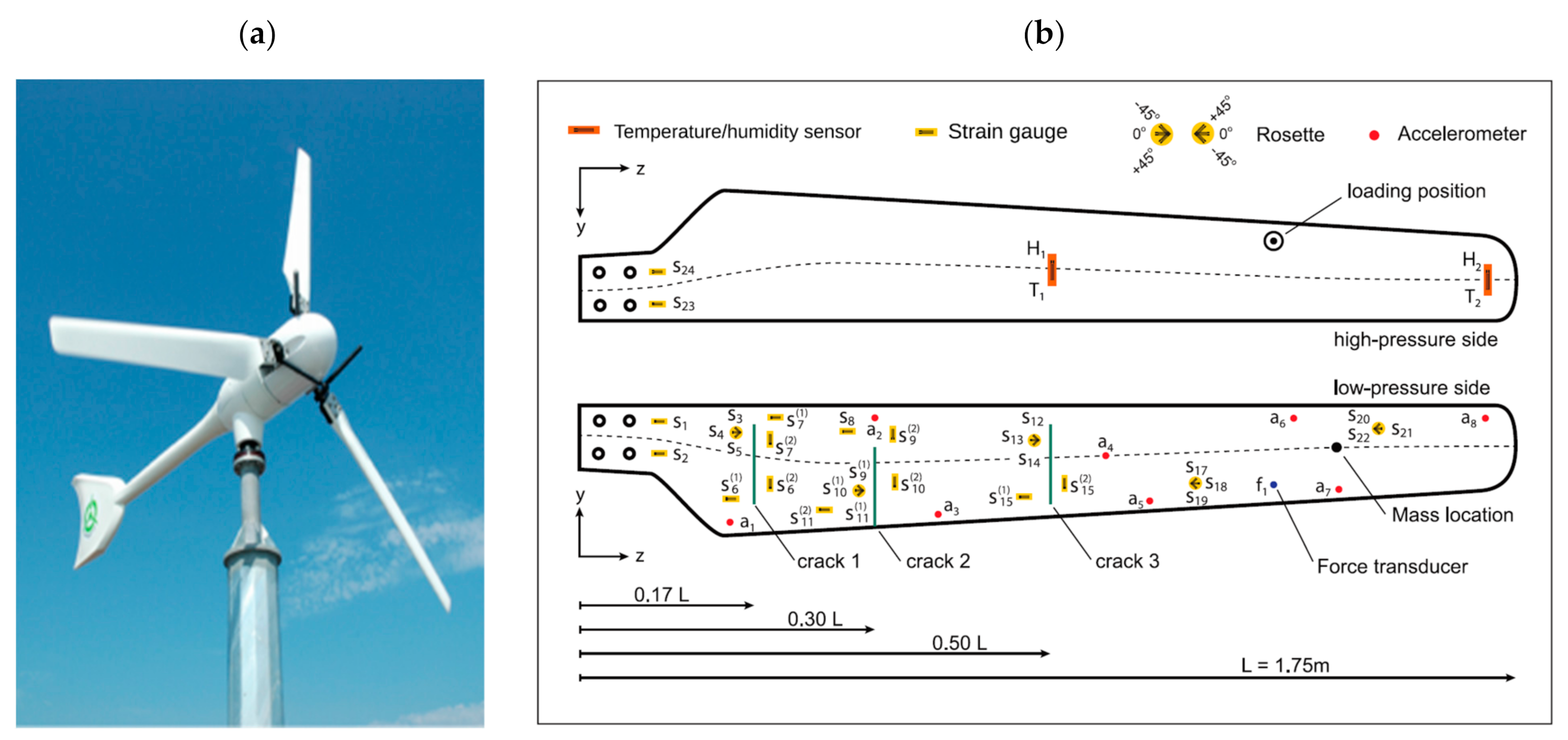
Ou et al. (2021) monitored a blade of a wind turbine model (Sonkyo-Energy-3.5 kW) under different excitation and environmental conditions. The length and mass of the Sonkyo-Energy-3.5 kW blade, as shown in Figure 4a,b, are 1.75 m and 5.0 kg, respectively. The blade was constructed based on a three-layered sandwich model using double-layered composite material, and more structural details of the model can be found in [58]. One end of the blade was connected to a steel frame using a fixed connection, and all the setup was assembled in a climate chamber where both temperature and humidity were controlled. Various temperatures were considered, varying from −15 °C to +40 °C, with a step increase of 5 °C to monitor the blade in different conditions. Different types of sensors, including eight accelerometers, were used to monitor the blade during the tests, and the locations of the sensors are presented in Figure 4b. Moreover, they developed the finite element model of the blade based on different scenarios and compared the results with the experimental results [63].

Two different types of excitations, including white noise and sine sweep signals with a duration of 120 s, were applied using an electromechanical shaker [58]. The measured data of the sine sweep signal (frequencies from 1 to 300 Hz) is considered in this case study. Two groups of damage scenarios were considered in several cases of the monitoring process, including icing conditions and cracks on the blade. Some lumped masses were used as the additional ice mass and applied on specific locations of the blade to simulate the icing conditions. Icing conditions are a common problem for wind turbines, as these structures are usually constructed in special locations. Moreover, some cuts on the blade with various lengths and locations in different cases were considered, and the details of each damage scenario are shown in

Table 2. Details of the controlled tests of the wind turbine blade [58].

Test Label	Description
R	Healthy State
A	Added mass 1 × 44 g
B	Added mass 2 × 44 g
C	Added mass 3 × 44 g
D	Crack 1: L1 = 5 cm
E	Crack 1: L1 = 5 cm	Crack 2: L2 = 5 cm
F	Crack 1: L1 = 5 cm	Crack 2: L2 = 5 cm	Crack 3: L3 = 5 cm
G	Crack 1: L1 = 10 cm	Crack 2: L2 = 5 cm	Crack 3: L3 = 5 cm
H	Crack 1: L1 = 10 cm	Crack 2: L2 = 10 cm	Crack 3: L3 = 5 cm
I	Crack 1: L1 = 10 cm	Crack 2: L2 = 10 cm	Crack 3: L3 = 10 cm
J	Crack 1: L1 = 15 cm	Crack 2: L2 = 10 cm	Crack 3: L3 = 10 cm
K	Crack 1: L1 = 15 cm	Crack 2: L2 = 15 cm	Crack 3: L3 = 10 cm
L	Crack 1: L1 = 15 cm	Crack 2: L2 = 15 cm	Crack 3: L3 = 15 cm

. For instance, C+25 refers to the test that is based on case C in Table 2 with a temperature of +25 °C.

4. System Identification

The selected structures, as shown in Section 3, are analyzed using SOBI and TVF-EMD, and the identified modal parameters are presented below.

4.1. Results Obtained from the Eeklo Pedestrian Bridge

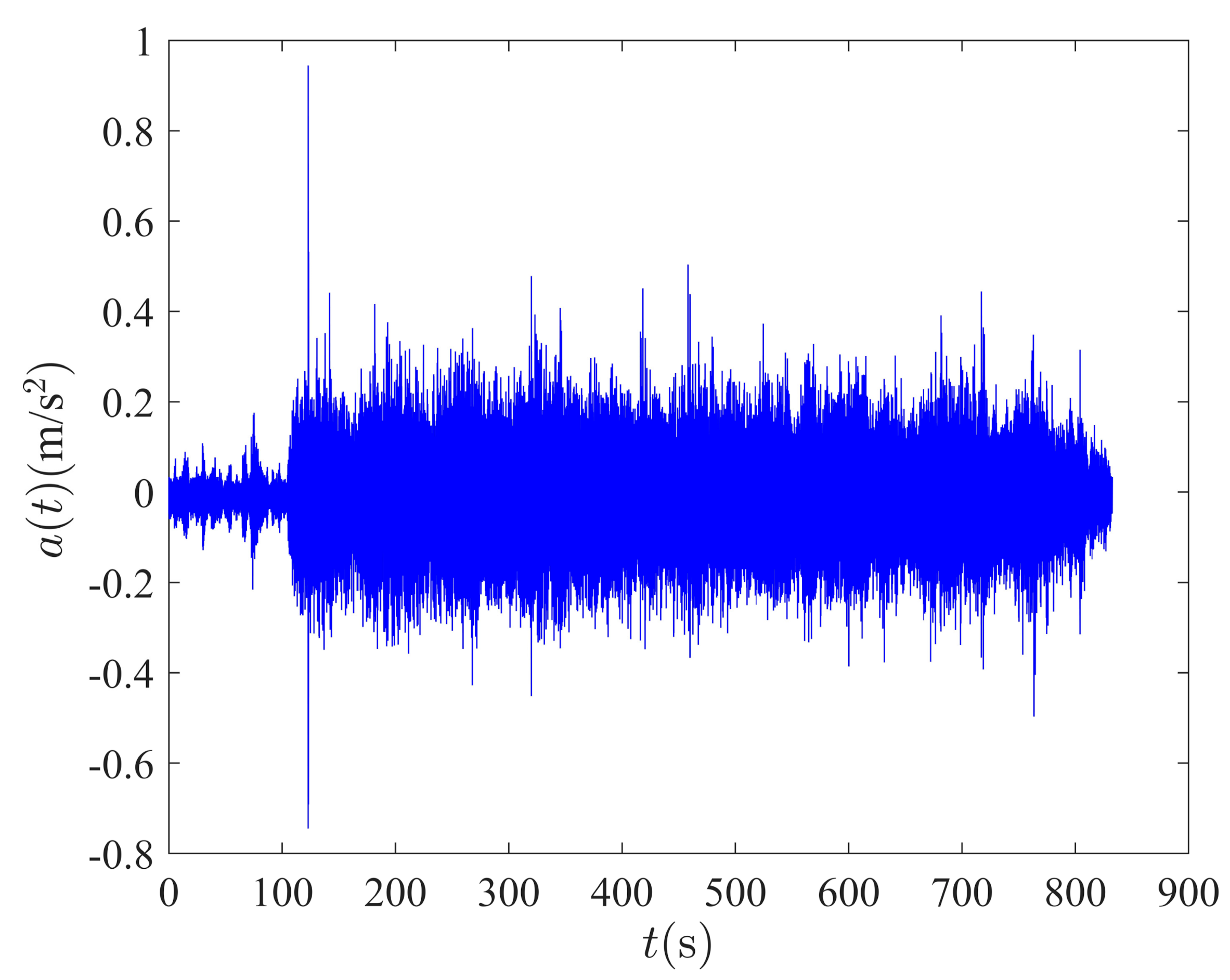
Before discussing the results of SOBI and TVF-EMD, the time-domain signal of the structure of test #A-2 is presented in Figure 5.

4.1.1. SOBI Method

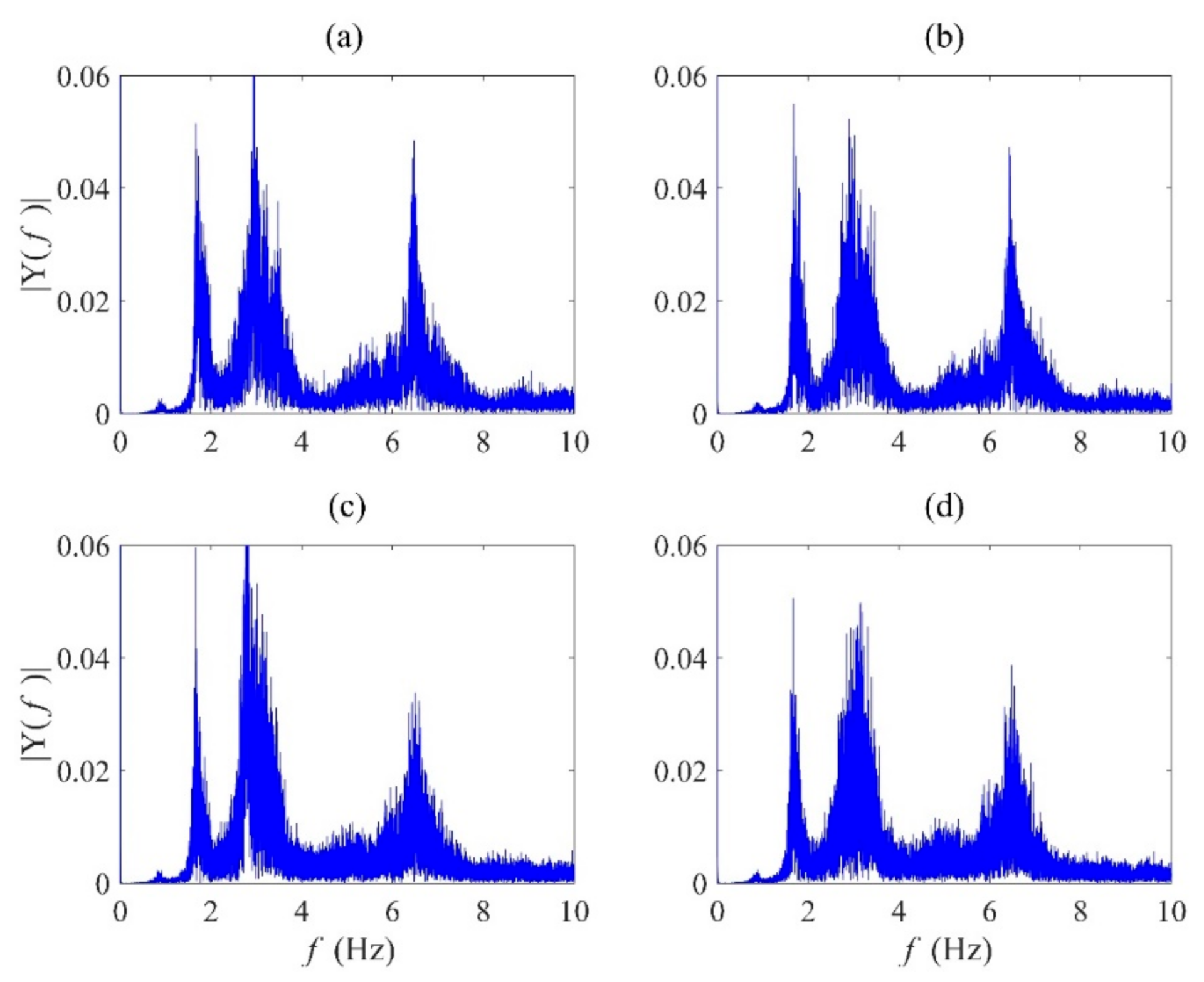
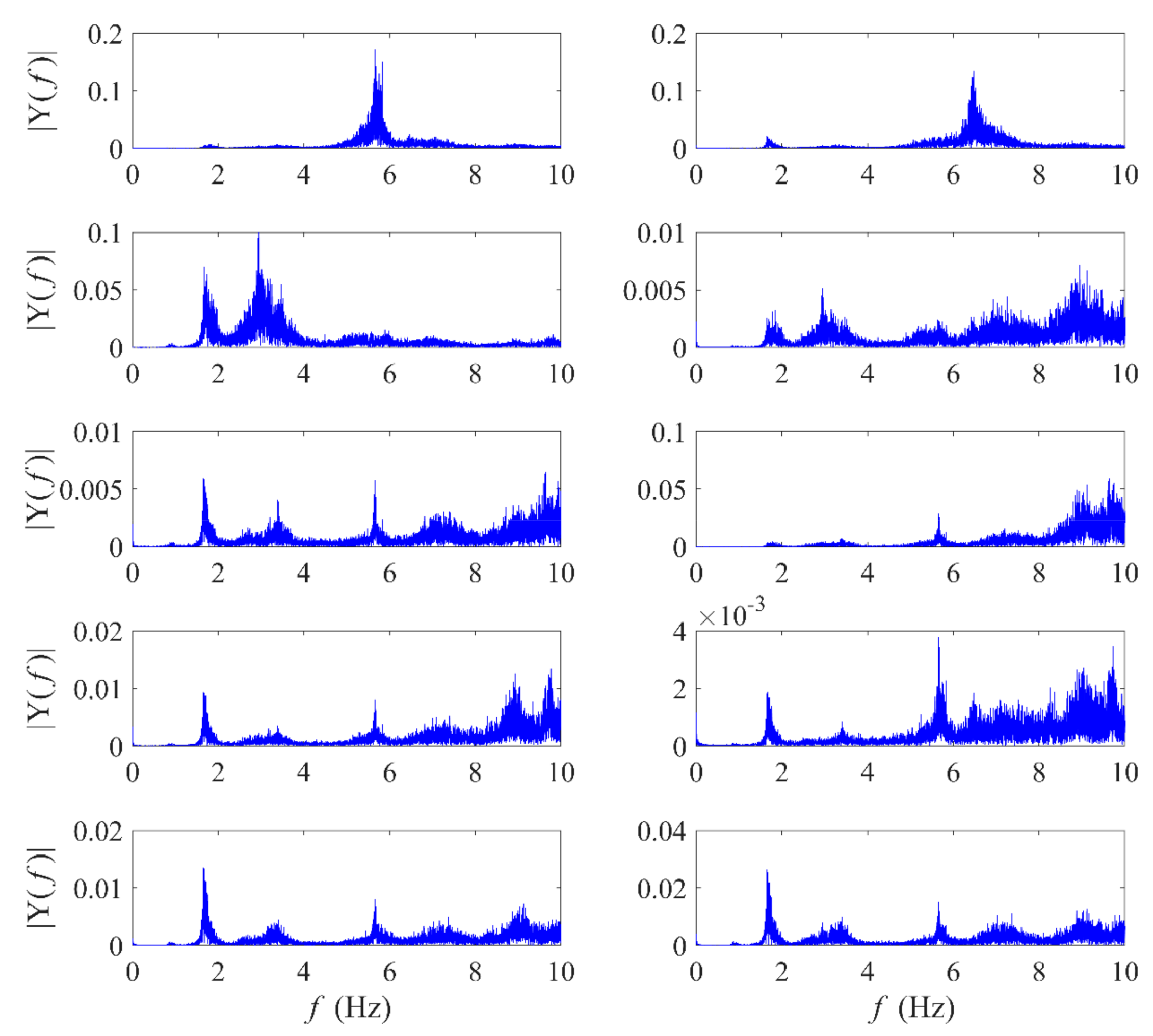
Van Nimmen et al. (2021) identified the first 12 modal frequencies of the Eeklo Bridge using experimental tests, as well as conducted FE simulations. Fourier spectra from the raw data of a few typical tests are presented in Figure 6, which can be compared with the modal frequencies of the bridge in

Table 3. Modal frequencies (Hz) of the Eeklo Pedestrian Bridge using SOBI.

	Mode #
Test #	1	2	3	4	5	6	7	8	9	10	11	12
FE [57]	1.69	2.97	3.21	3.44	5.68	5.74	6.01	6.42	6.98	7.44	9.64	9.89
SSI [57]	1.71	2.99	3.25	3.46	5.77	5.82	6.04	6.47	6.98	7.44	9.64	9.89
A-A	1.69	2.97				5.74		6.42
A-1	1.69	2.95			5.65			6.52
A-2	1.67				5.67			6.44
A-3	1.67				5.66			6.46
A-4	1.71				5.67			6.41
B-B	1.67	2.97						6.42
B-1	1.66				5.66			6.43
B-2	1.67				5.67			6.47
B-3	1.63				5.69			6.45
B-4	1.66				5.71			6.47			9.56

. As shown, just modes 1.69, 2.97, and 6.42 Hz have enough energy in all cases to be identified, and these modal frequencies have good agreement with the identified modal frequencies by Van Nimmen et al. (2021). The data of all ten tests conducted on the bridge have been analyzed by the SOBI technique, where data from all the sensors have been considered for analysis. For instance, the output of the mode identification of the A-1 test using SOBI is presented in Figure 7. As shown, only four sources show clear modal responses, and the rest are mode-mixed or repeated. Therefore, just the modal responses of four frequencies are identified for the A-1 test. The rest of the modes were not recognized due to insufficient energy in the time-domain data.

One limitation of SOBI is that the maximum number of the identified source components remains the number of sensors. Hence, as a total of ten sensors were used, the results of the SOBI method are limited to ten regardless of the number of modes. Therefore, as the bridge has 12 modes within 0–10 Hz, mode-mixing has resulted in the identified modal responses. As summarized in Table 3, SOBI can identify just 3–4 modes out of 12 modes of the structures using Equation (11). Moreover, comparing different tests in Table 3 confirms that the type of excitation, including ambient and pedestrian excitations, does not have a considerable effect on the performance of the SOBI method. For instance, the results of A-A and A-2 tests have 4 and 3 identified modes, respectively, although these tests are totally different regarding the type of excitation. It may also be concluded that additional sensors could have improved the performance of SOBI for such a large-scale structure.

4.1.2. TVF-EMD Method

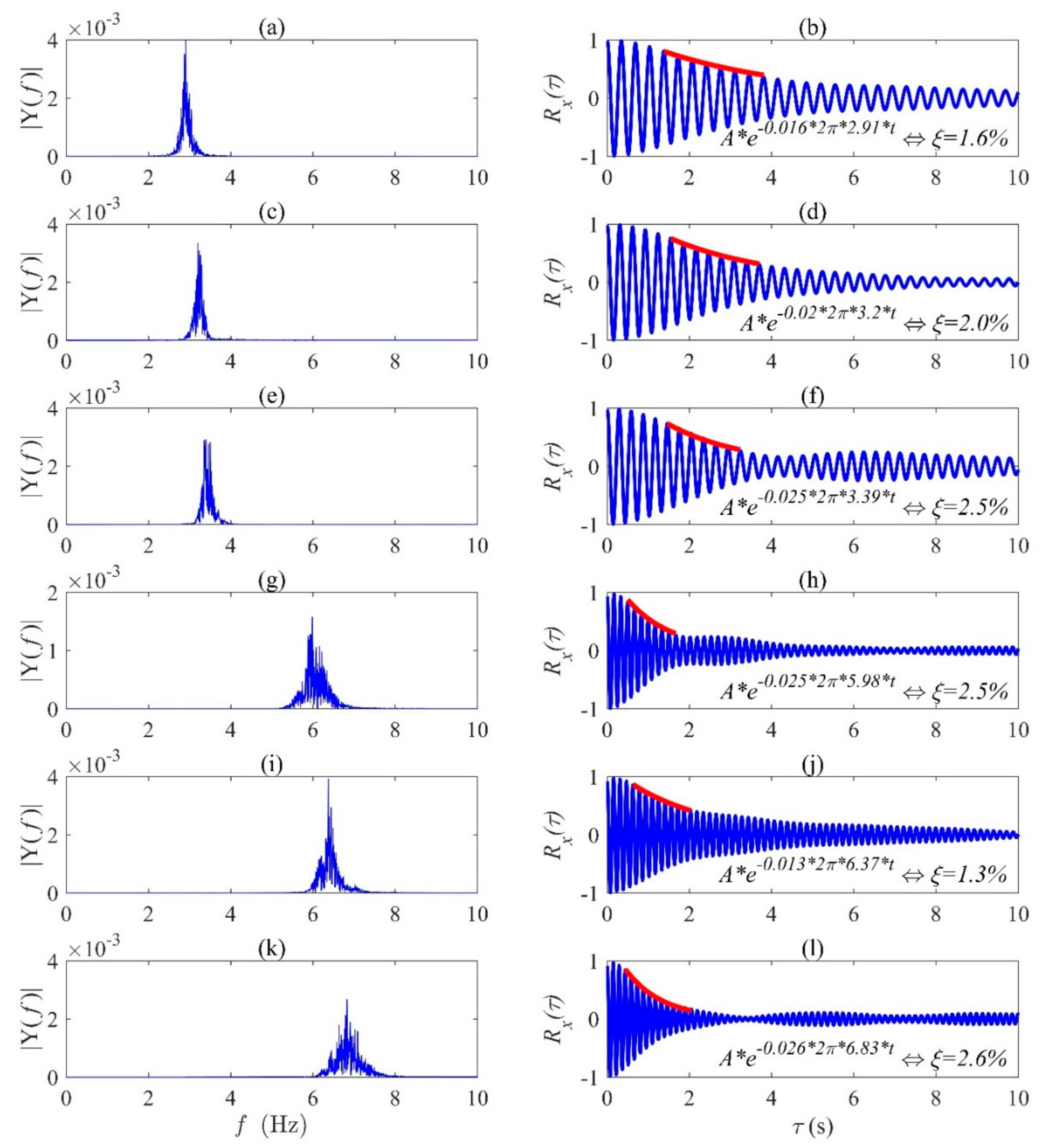
The TVF-EMD method is explored next for the modal identification of the test bridge. The damping ratios of the structure corresponding to the IMFs are estimated using the Auto-Correlation Function (ACF), followed by the exponential fitting. Figure 8 shows the modal frequencies and the corresponding damping ratio of the middle sensor data of test #A-2, which was obtained based on Equations (16) and (17). Figure 8a,c,e,g,i,k are the resulting Fourier spectra of the IMFs of the identified modal frequencies of the structure. Figure 8b,d,f,h,j,l illustrate the corresponding damping ratios obtained from the decay curve of their ACF.

Table 4. Modal frequencies (Hz) of the Eeklo Pedestrian Bridge using TVF-EMD based on its mid-span sensor.

	Mode #
Test #	1	2	3	4	5	6	7	8	9	10	11	12
FE [57]	1.69	2.97	3.21	3.44	5.68	5.74	6.01	6.42	6.98	7.44	9.64	9.89
SSI [57]	1.71	2.99	3.25	3.46	5.77	5.82	6.04	6.47	6.98	7.44	9.64	9.89
A-A	1.69	2.97	3.22	3.45	5.66	5.74		6.42				9.89
A-1	1.72	2.95		3.45	5.70			6.48				9.77
A-2		2.91	3.20	3.39			5.98	6.37	6.83
A-3		3.01	3.18	3.49	5.66	5.86	5.93	6.43	6.94		9.61	9.85
A-4		2.99	3.15	3.49	5.72	5.82	6.10	6.43	6.87
B-B		2.97					5.90
B-1	1.67	2.88	3.29	3.59				6.55	7.01			9.86
B-2	1.68	2.95	3.10	3.37	5.47	5.80	5.94	6.43	7.04
B-3	1.64	3.00	3.25		5.45		5.90	6.50	7.19			9.89
B-4	1.64	2.90	3.11	3.57				6.52	7.14

presents the modal frequencies (Hz) of the bridge using TVF-EMD by considering its middle sensor. As shown, except for test #A-A, at least 6 out of 12 modes of the structural modes have been identified using this method. Even in some cases, such as test #A-3, 10 out of 12 modes have been identified, confirming the efficiency of the TVF-EMD method.

By comparing Table 3 and Table 4, it can be concluded that the TVF-EMD method is more efficient than the SOBI method for the modal identification of closely-spaced frequency structures, as TVF-EMD results in more identified modal frequencies. As shown in Table 3 and Table 4, ~30% of the modes can be identified using SOBI, regardless of the type of the tests; however, the TVF-EMD method results in excellent identification accuracy. Moreover, the efficiency of the TVF-EMD method depends on the type of excitation, including ambient and pedestrian excitations, as the performance of this method is different depending on the excitation cases. On the other hand, the type of excitations does not affect the performance and accuracy of the SOBI method. The damping ratios of the structure corresponding to the IMFs are estimated using ACF and Equation (17), followed by the exponential fitting, and the results are shown in

Table 5. Estimated damping ratios (%) of the Eeklo Pedestrian Bridge corresponding to the identified modal frequencies using TVF-EMD.

	Mode Number (j)
Test #	1	2	3	4	5	6	7	8	9	10	11	12
SSI & FE [57]	1.94	0.19	1.45	2.97	0.23	0.16	2.08	0.60	3.38	4.77	0.87	2.50
A-A	1.75	0.77	2.67	1.45	2.15	0.62		0.63				2.65
A-1	2.35	1.55		2.60	3.25			1.65				2.67
A-2		1.59	2.02	2.52			2.48	1.28	2.60
A-3		1.49	2.40	2.71	2.08	2.79	2.69	1.40	3.21		2.67	2.95
A-4		1.58	1.71	2.02	2.47	2.20	2.93	1.65	2.02
B-B		0.19					2.51
B-1	6.90	1.80	3.49	3.20				1.69	1.64			1.16
B-2	11.32	2.99	6.14	5.65	3.48	3.28	2.96	1.72	2.70
B-3	11.31	2.90	5.58		3.39		2.84	1.65	2.57			1.87
B-4	10.61	2.72	5.57	4.86				1.48	2.43

. As can be seen in some cases, not only are the estimated damping ratios corresponding to the IMFs almost the same as the presented damping ratios by Van Nimmen et al. (2021), but also the damping ratios estimated based on different test data are nearly the same. However, the uncertainties in damping estimates are prevalent in the presence of closely-spaced modes, which can also be found in the literature [64].

4.2. Results Obtained from the Wind Turbine

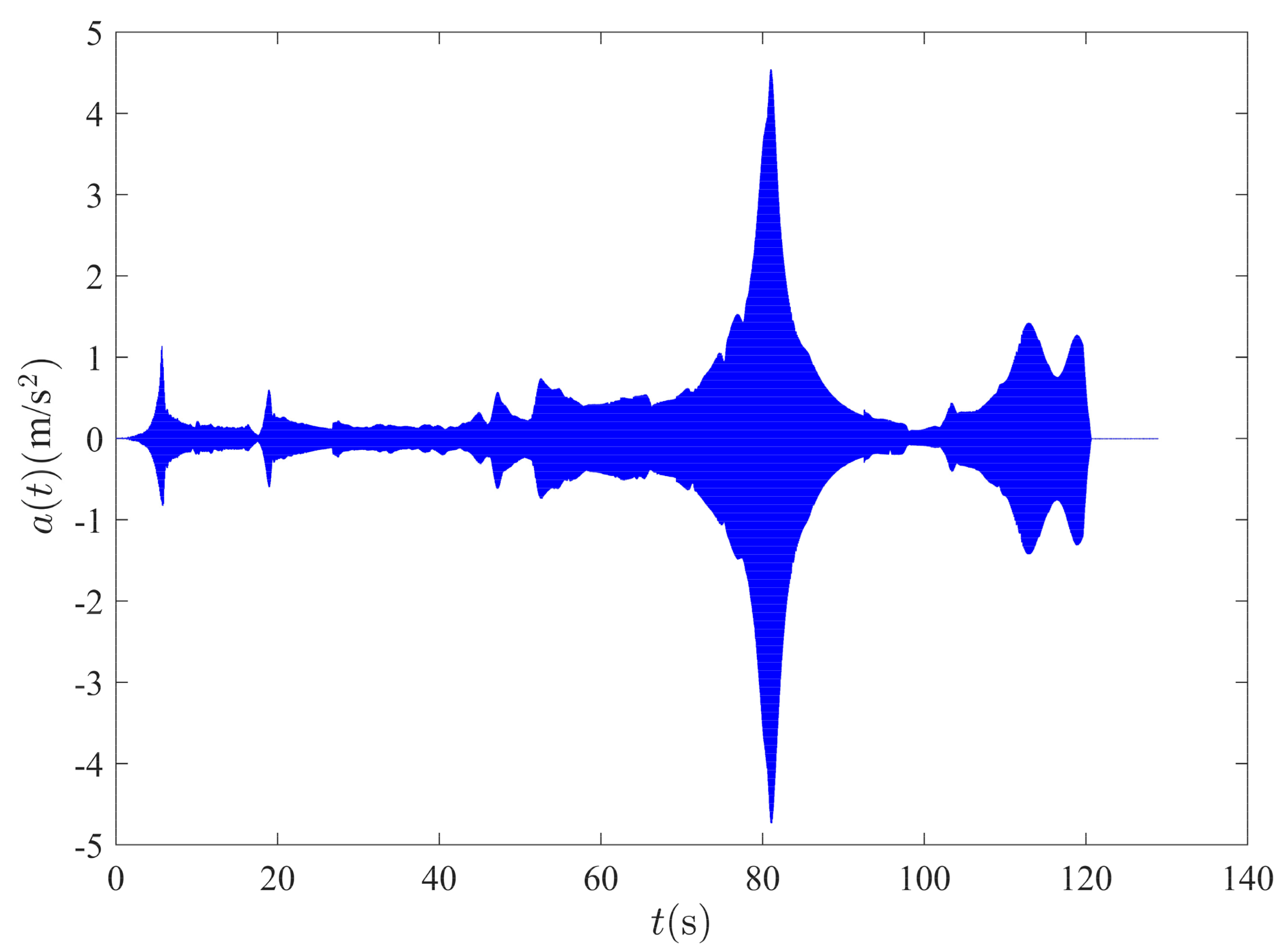
The time-domain signal of the wind turbine of test #A-2 is presented in Figure 9.

4.2.1. SOBI Method

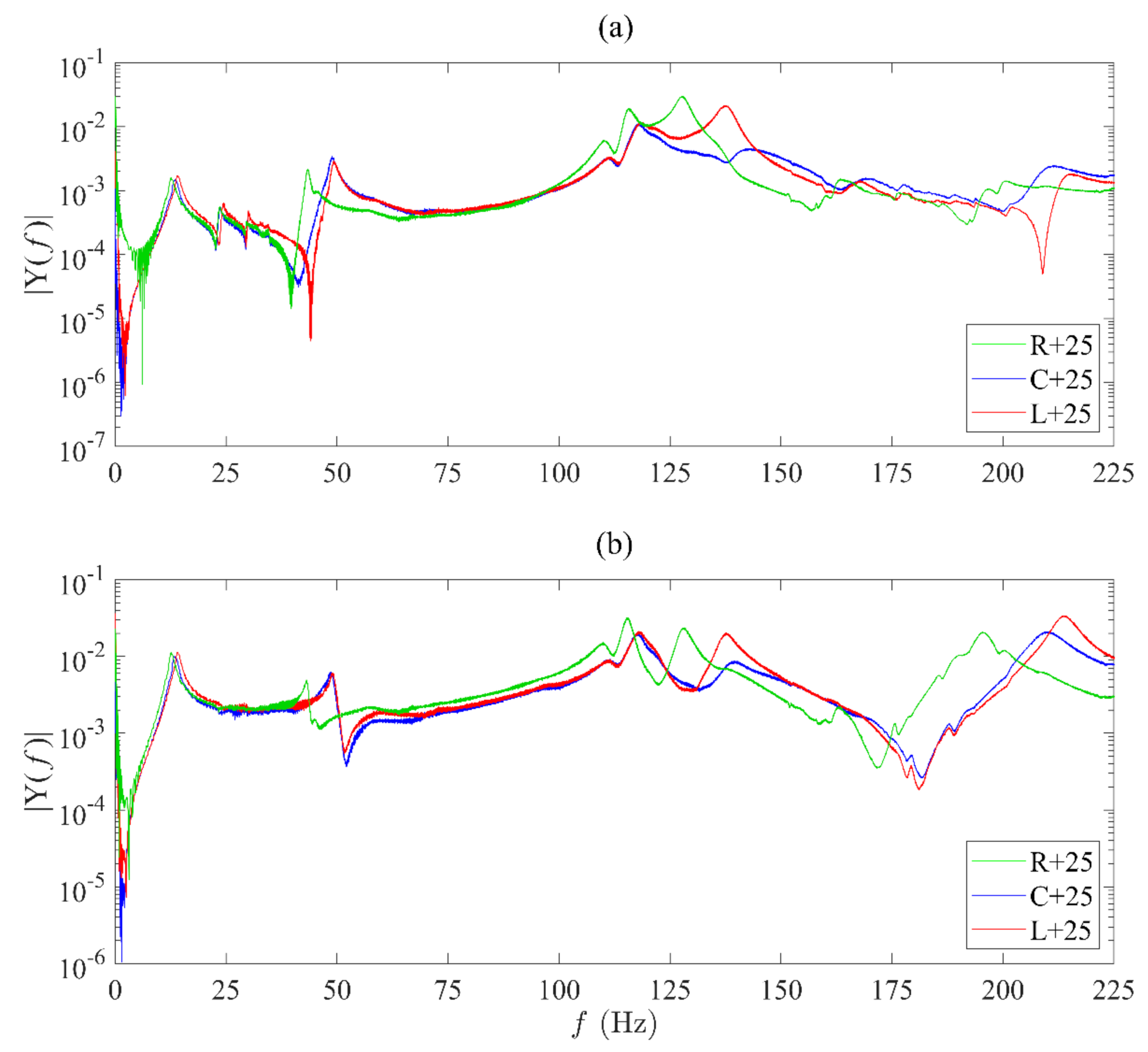
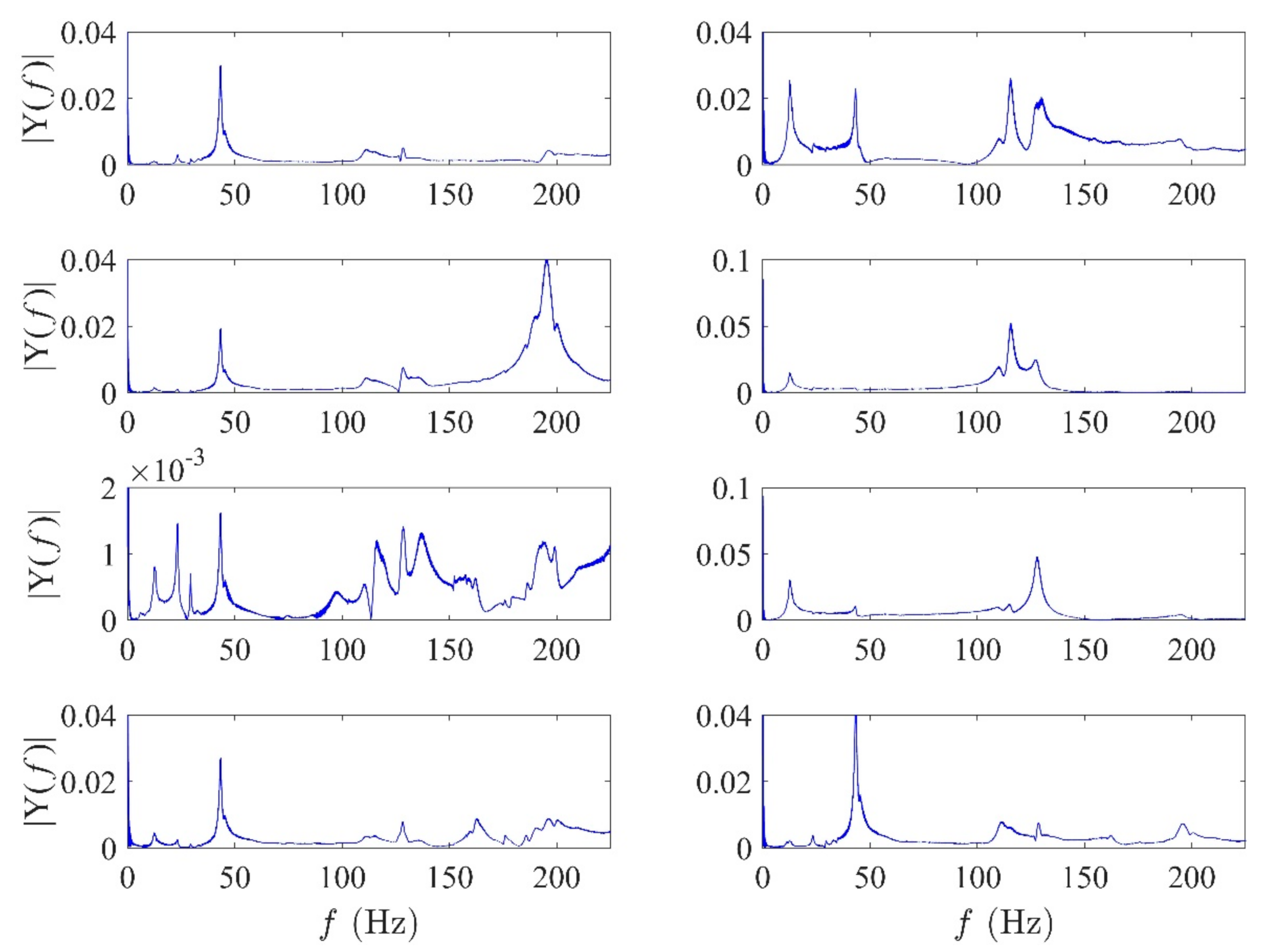
Ou et al. (2021) identified the first five modal frequencies of the blade using the SSI method by considering all eight sensors. The first three modes and the following two modes are longitudinal and torsional, respectively. As discussed in Section 3, eight accelerometers, a₁ to a₈, were used to monitor the blade, and the Fourier spectra of the data collected from a₃ and a₈ are shown in Figure 10, which prove the identified modal frequencies by Ou et al. (2021). The output of SOBI applied on different types of tests, which were calculated based on Equation (11)—including healthy state (R+25), added mass damage scenario (C+25), and cracked blade damage scenario (L+25)—are presented in Figure 11, Figure 12 and Figure 13, respectively. By comparing these figures, it can be mentioned that the accuracy and performance of the SOBI do not depend on the type of the tests and damage scenarios. For instance, in Figure 13, the second, third, and fifth modes of the structure are clear; however, the rest of the components have mixed modes.

The first five identified modal frequencies of the blade using SSI are presented in

Table 6. Identified modal frequencies (Hz) of the wind turbine blade at +25 °C using the SOBI method.

	Mode #
Test #	1	2	3	4	5
SSI [58]	13.41	47.03	117.45	135.60	207.99
R	-	49.19	118.13	137.38	213.57
A	-	49.18	-	137.04	-
B	13.74	48.85	-	-	211.47
C	13.71	48.86	118.47	-	209.57
D	-	49.03	117.59	137.13	213.35
E	-	48.80	117.37	-	211.87
F	13.89	-	117.39	-	210.64
G	-	47.96	117.49	135.57	209.59
H	-	48.16	116.76	-	207.68
I	14.68	46.36	-	-	-
J	14.06	-	116.44	131.54	-
K	12.62	-	116.11	-	201.13
L	-	43.34	115.47	-	-

. Moreover, the data from all cases, including health state and damage scenarios at a temperature of +25 °C (added masses and cracks), are analyzed using SOBI, which is shown in Table 6. As illustrated, the SOBI method can identify 40–80% of the modes of the wind turbine blade throughout the different tests. Moreover, by comparing one of the modes of the structure in different tests in Table 6, for example, the third mode of the structure, the more added mass and cracks, the smaller modal frequency. Regardless of the type of tests and damage scenarios, almost, in most cases, 60% of the modes are identified, which is more accurate than the results of the SOBI method applied on the Eeklo Pedestrian Bridge. As shown in Table 3, SOBI could identify nearly 30% of the modes of the Eeklo Pedestrian Bridge regardless of the type of excitation and conditions.

The reason for this considerable variation in the performance of the SOBI method could be due to the difference in the number of sensors used to monitor the structures. For the Eeklo Pedestrian Bridge, 10 sensors have been used to identify 12 modes. However, eight sensors have been considered to identify just five modes of the wind turbine blade. As mentioned, the limitation of the SOBI technique is that the maximum number of the identified source components will be the number of sensors. From this, it can be concluded that the SOBI method is more efficient when the number of channels is more than the number of modes that should be identified. Moreover, the SSI method used in [58] requires an intensive stabilization diagram and model order selection. This tedious process is not required in either SOBI or TVF-EMD, which is the advantage of these methods over SSI.

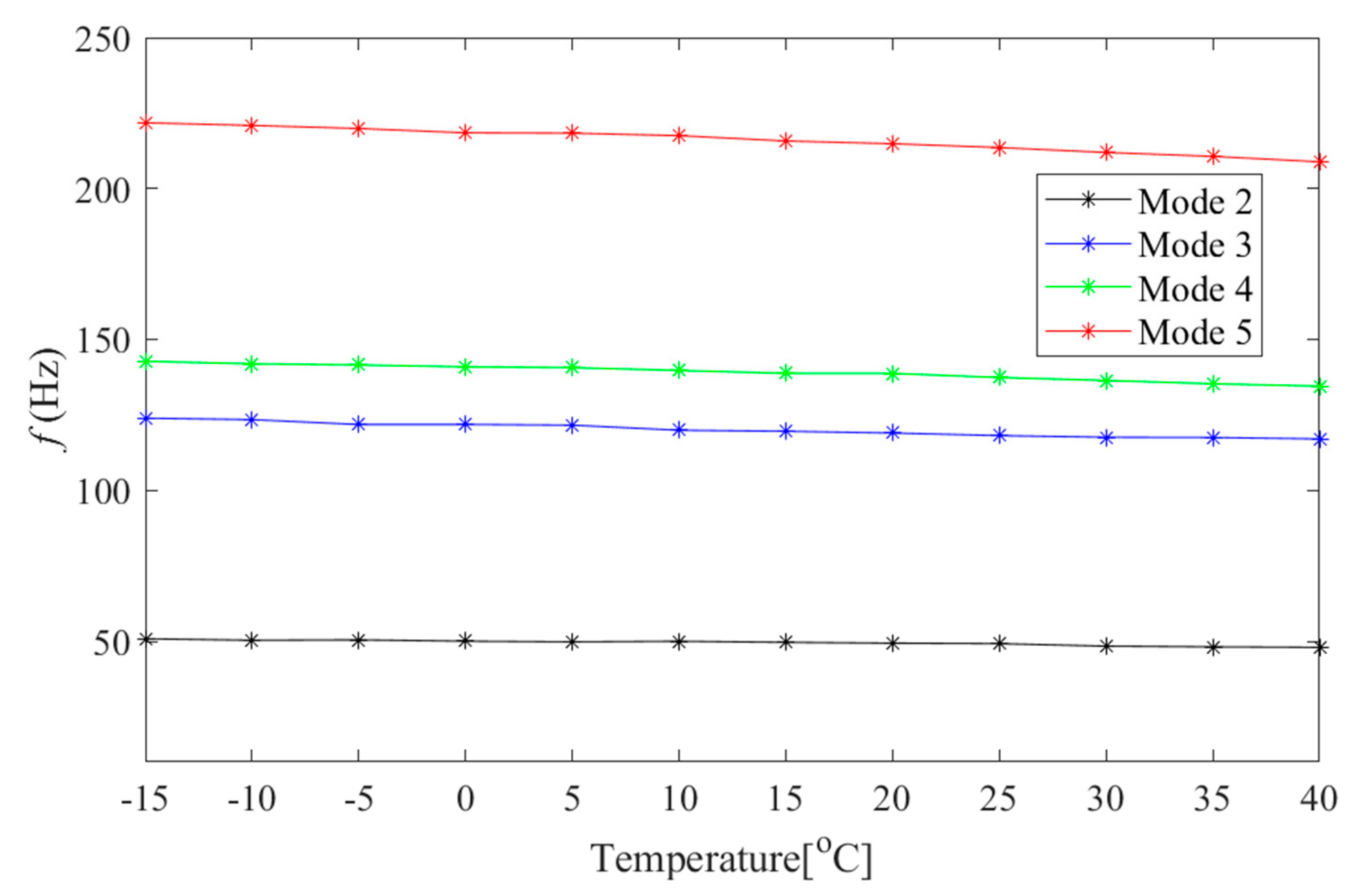
To assess the effects of the blade temperature on the results and performance of the SOBI method for modal identification, the results of test R at different temperatures, varying from −15 °C to +40 °C and considering a step of 5 °C, have been analyzed and the identified frequencies are presented in Figure 14. As shown, as the temperature increases, the frequency of the mode decreases linearly. By comparing the results of different modes, the frequencies of the fifth and second modes decrease by 0.24 Hz and 0.05 Hz per unit temperature (°C), respectively. Hence, changing the temperature does not equally affect the identified frequencies of the different modes. For instance, if the frequency of the modes of the wind turbine blade is less than 100 Hz, the effect of temperature is negligible.

4.2.2. TVF-EMD Method

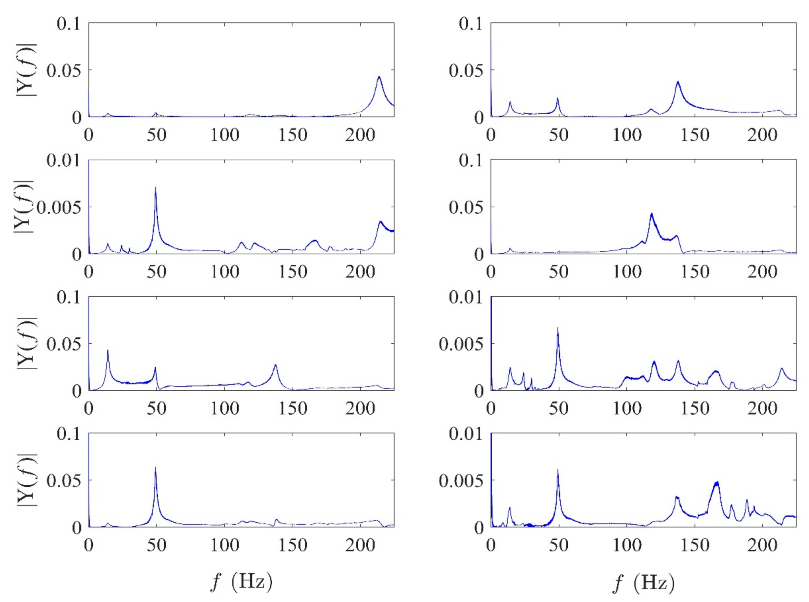
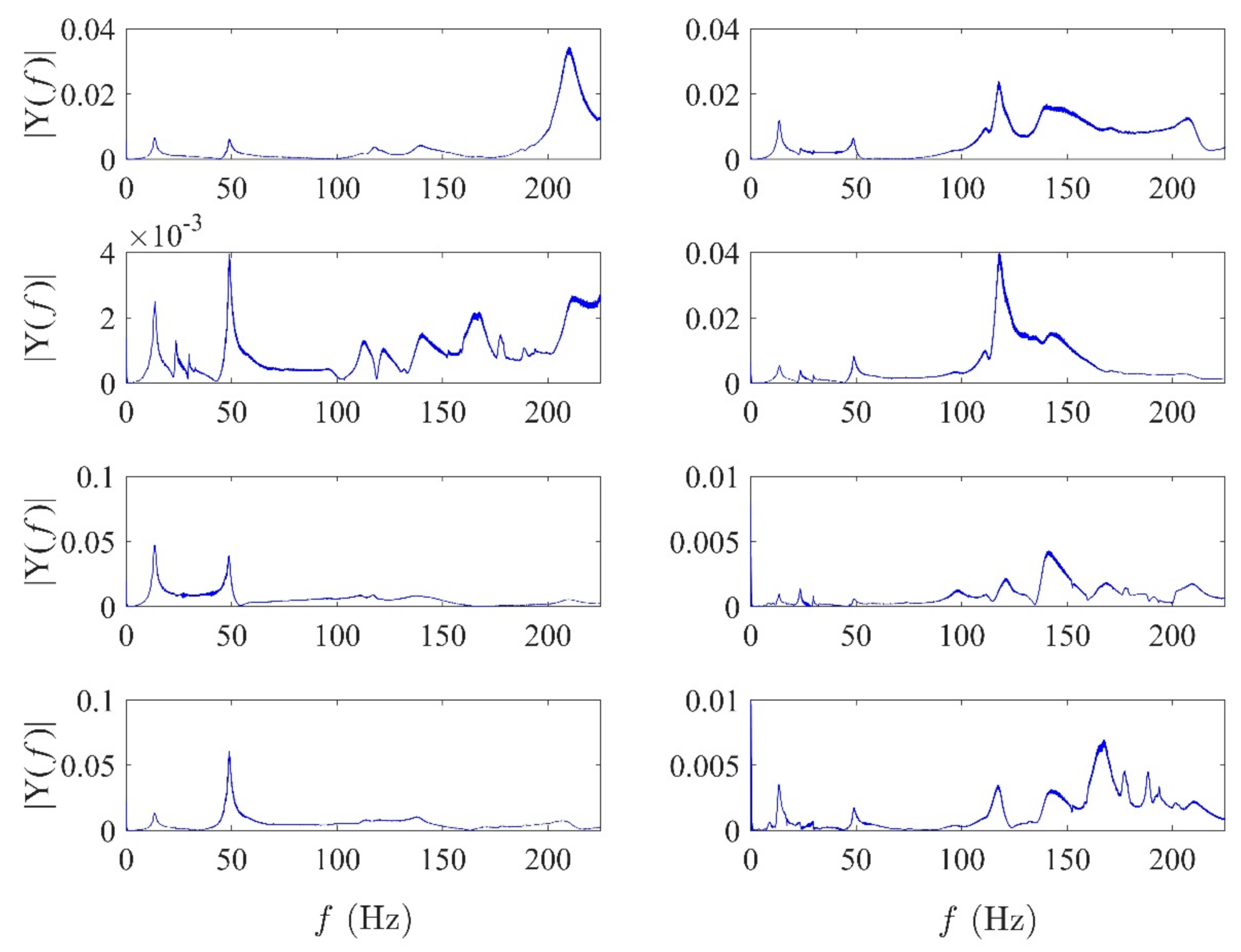
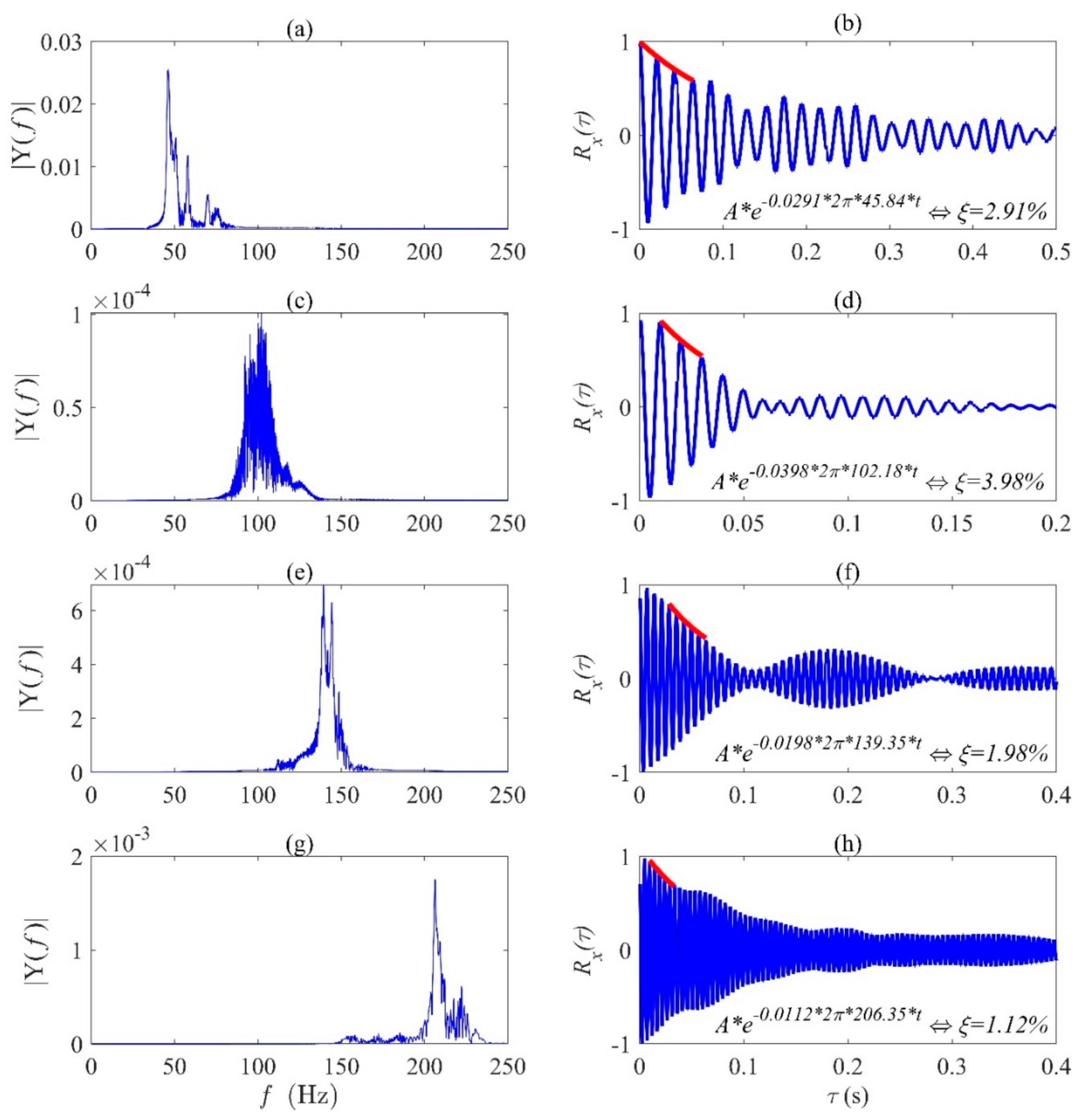
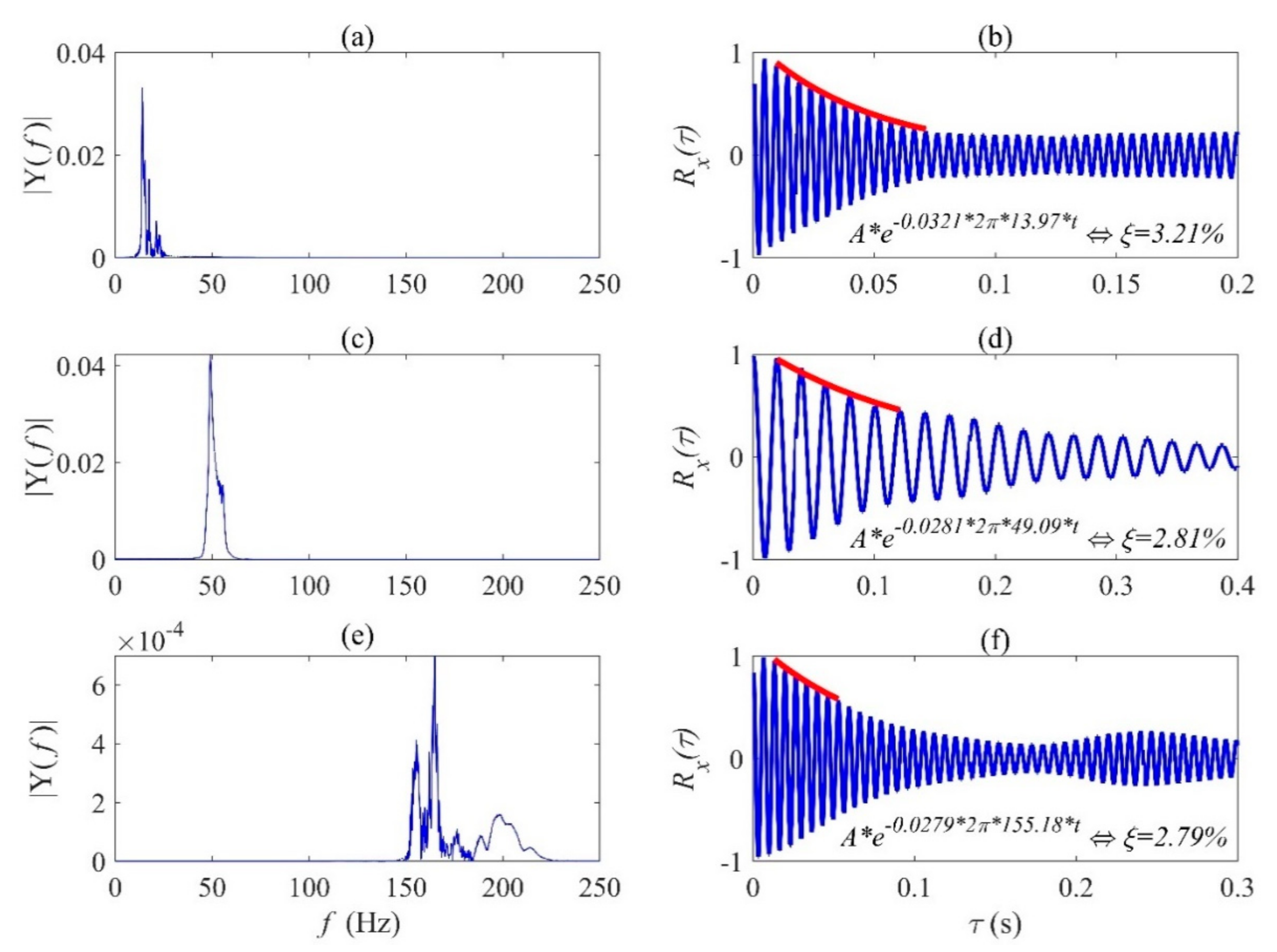
The TVF-EMD method has been used for a similar analysis of the wind turbine blade data. Moreover, the damping ratios of the structure corresponding to the IMFs are estimated using ACF followed by the exponential fitting using Equation (17). For example, modal frequencies and the corresponding damping ratios of the test# K and B are presented in Figure 15 and Figure 16. Figure 15a,c,e,g and Figure 16a,c,e are the Fourier spectra of the IMFs of the identified modal frequencies of the structure using the TVF-EMD method. As shown, four IMFs in Figure 15 and three IMFs in Figure 16 present four and three modes out of five modes of the structure, respectively. Figure 15b,d,f,h and Figure 16b,d,f illustrate the corresponding damping ratios obtained from the decay curve of their ACF. As shown, based on the data of test K, modes 2, 3, 4, and 5 have been identified. Also, according to the data of test# B, modes 1, 2, and 4 have been identified.

The modal identification results using the a₄ sensor at the middle of the blade at +25 °C are shown in

Table 7. Identified modal frequencies (Hz) of the wind turbine blade at +25 °C using TVF-EMD by considering a₄.

	Mode #
Test #	1	2	3	4	5
SSI [58]	13.41	47.03	117.45	135.60	207.99
R	-	49.42	-	156.52	215.35
A	-	49.25	-	147.51	214.44
B	13.97	49.09	-	155.18	-
C	14.23	-	-	167.93	215.10
D	-	49.34	-	-	203.27
E	-	49.00	-	159.35	209.01
F	14.68	52.25	113.85	-	-
G	-	47.42	103.26	149.76	210.60
H	-	49.25	95.60	152.85	206.69
I	-	44.67	-	153.85	205.44
J	-	47.00	-	151.85	210.60
K	-	46.25	102.18	139.15	206.35
L	15.34	-	-	143.10	-

. From this, it can be concluded that the TVF-EMD method can identify 40–80% of the modes of the blade in different cases. In most cases, at least three modes out of five modes (i.e., 60% of the modes) have been identified. By comparing Table 6 and Table 7, it can be noted that the accuracy of both SOBI and TVF-EMD are almost the same. In most cases, both methods identified 60% of the modal frequencies of the wind turbine blade. On the other hand, TVF-EMD had a better performance than SOBI for modal identification of the Eeklo Pedestrian Bridge, as discussed in Table 3 and Table 4. The reason for this difference can be the shortage of channels and sensors in the modal identification of the bridge (10 sensors versus 12 modes). From this, it can be concluded that if the number of sensors is less than the number of target modes of the structure, TVF-EMD will have better performance and higher accuracy than the SOBI method.

On the other hand, when the number of sensors is equal to or more than the number of modes of the structure, TVF-EMD and SOBI will have almost the same performance. In these cases, the SOBI method will be the better choice, as this analysis takes less time than the TVF-EMD method. The average run-time of both methods in different cases of the case studies is presented in

Table 8. The average run-time of the methods in both case studies.

	Run Time (min)
Case Study	TVF-EMD	SOBI
Eeklo Pedestrian Bridge	38.20	0.13
Wind turbine blade	29.40	0.10

. The MATLAB codes were run by a computer with a Core-i7 CPU. As shown, the run-time of TVF-EMD is 287-times (average) more than the run-time of the SOBI method, which proves the advantage of SOBI in this regard. The damping ratios of the structure corresponding to the IMFs are estimated using ACF followed by the exponential fitting, and the results are shown in

Table 9. Estimated damping ratios of the wind turbine blade corresponding to the identified modal frequencies by the TVF-EMD method.

	Mode #
Test Label (+25 °C)	1	2	3	4	5
R	-	3.49	-	0.74	1.00
A	-	3.10	-	1.11	0.39
B	3.21	2.81	-	2.79	-
C	2.11	-	-	1.08	1.68
D	-	3.24	-	-	2.52
E	-	1.21	-	2.21	1.34
F	3.13	2.89	2.84	-	-
G	-	3.53	3.78	7.82	1.08
H	-	1.11	3.02	0.52	0.78
I	-	3.01	-	1.41	1.52
J	-	2.18	-	1.13	1.46
K	-	2.91	3.98	1.98	1.12
L	1.25	-	-	0.72	-

. The damping ratios estimated based on different test data are almost the same. For example, the damping ratio of the third mode is around 3% in different tests.

5. Conclusions

A comprehensive study has been implemented to validate the accuracy of TD and TFD modal identification methods, SOBI and TVF-EMD, and compare their performance. These techniques have been applied to analyze the structural monitoring data of two full-scale structures, the Eeklo Pedestrian Bridge and Sonkyo wind turbine blade, subjected to different excitations and damage scenarios. The outputs of each method for different cases and tests have been presented and compared. The following conclusions can be drawn:

• SOBI has identified 25–33% of the modes of the Eeklo Pedestrian Bridge and 40–80% (60% in most cases) of the modes of the wind turbine blade in different cases. The reason for this considerable variation could be due to the difference in the number of channels used to monitor the structures. For the Eeklo Pedestrian Bridge, 10 sensors have been used to identify 12 modes. However, eight sensors have been considered to identify five modes of the wind turbine blade. Since the limitation of the SOBI technique is that the maximum number of the identified source components will be the number of sensors, the accuracy of the SOBI method is improved when the number of channels is more than the number of target modes. On the other hand, the TVF-EMD method could identify 50–83% of the Eeklo Bridge modes and 40–80% of the wind turbine blade modes in different cases. Hence, the accuracy of this method does not depend on the type of structure, the number of channels, and the number of modes of the structure.
• If the number of sensors is less than the number of modes of the structure, TVF-EMD will have better performance and higher accuracy than the SOBI method.
• When the number of sensors is equal to or more than the number of modes of the structure, TVF-EMD and SOBI have almost the same performance. In these cases, the SOBI method will be the better choice, as this analysis takes less time than the TVF-EMD method. In all tests of these case studies, SOBI takes less than one minute; however, TVF-EMD takes 34 min on average, which is considerably more than the run-time of SOBI.
• The performance of the SOBI method is independent of the type of excitation, including ambient- and pedestrian-induced excitations, and the type of damage scenarios. It could identify almost the same percentage of the modes in different tests conducted on the structures. On the other hand, the type of damage scenario and excitations affect the TVF-EMD accuracy considerably.
• As the temperature increases, the frequency of the modes decreases linearly. Moreover, the effects of temperature on the modes with higher frequencies are more than the modes with lower frequencies.
• The estimated damping ratios using ACF corresponding to the IMFs identified by TVF-EMD method have a good agreement with the damping ratios of the structure. Also, the damping ratios estimated based on different test data are almost the same. Therefore, the different excitation and damage scenarios do not affect the estimated damping ratios.

References

- Momeni, H.; Ebrahimkhanlou, A. High-dimensional data analytics in structural health monitoring and non-destructive evaluation: A review paper. Smart Mater. Struct. 2022, 31, 043001. [Google Scholar] [CrossRef]
- Su, J.; Xia, Y.; Weng, S. Review on field monitoring of high-rise structures. Struct. Control Health Monit. 2020, 27, e2629. [Google Scholar] [CrossRef]
- Sony, S.; Laventure, S.; Sadhu, A. A literature review of next-generation smart sensing technology in structural health monitoring. Struct. Control Health Monit. 2019, 26, e2321. [Google Scholar] [CrossRef]
- Eshkevari, S.S.; Matarazzo, T.J.; Pakzad, S.N. Bridge modal identification using acceleration measurements within moving vehicles. Mech. Syst. Signal Process. 2020, 141, 106733. [Google Scholar] [CrossRef] [Green Version]
- Hou, R.; Xia, Y. Review on the new development of vibration-based damage identification for civil engineering structures: 2010–2019. J. Sound Vib. 2021, 491, 115741. [Google Scholar] [CrossRef]
- Singh, P.; Keyvanlou, M.; Sadhu, A. An improved time-varying empirical mode decomposition for structural condition assessment using limited sensors. Eng. Struct. 2021, 232, 111882. [Google Scholar] [CrossRef]
- Tang, T.; Yang, D.-H.; Wang, L.; Zhang, J.-R.; Yi, T.-H. Design and application of structural health monitoring system in long-span cable-membrane structure. Earthq. Eng. Eng. Vib. 2019, 18, 461–474. [Google Scholar] [CrossRef]
- Sun, L.; Shang, Z.; Xia, Y.; Bhowmick, S.; Nagarajaiah, S. Review of bridge structural health monitoring aided by big data and artificial intelligence: From condition assessment to damage detection. J. Struct. Eng. 2020, 146, 04020073. [Google Scholar] [CrossRef]
- Zhang, L.; Qiu, G.; Chen, Z. Structural health monitoring methods of cables in cable-stayed bridge: A review. Measurement 2021, 168, 108343. [Google Scholar] [CrossRef]
- Yang, R.; He, Y.; Zhang, H. Progress and trends in nondestructive testing and evaluation for wind turbine composite blade. Renew. Sustain. Energy Rev. 2016, 60, 1225–1250. [Google Scholar] [CrossRef]
- Chandrasekhar, K.; Stevanovic, N.; Cross, E.J.; Dervilis, N.; Worden, K. Damage detection in operational wind turbine blades using a new approach based on machine learning. Renew. Energy 2021, 168, 1249–1264. [Google Scholar] [CrossRef]
- Beale, C.; Niezrecki, C.; Inalpolat, M. An adaptive wavelet packet denoising algorithm for enhanced active acoustic damage detection from wind turbine blades. Mech. Syst. Signal Process. 2020, 142, 106754. [Google Scholar] [CrossRef]
- ASCE. A Comprehensive Assessment of America’s Infrastructure—Report Card; American Society of Civil Engineers (ASCE): Reston, VA, USA, 2021. [Google Scholar]
- Lian, J.; Cai, O.; Dong, X.; Jiang, Q.; Zhao, Y. Health monitoring and safety evaluation of the offshore wind turbine structure: A review and discussion of future development. Sustainability 2019, 11, 494. [Google Scholar] [CrossRef] [Green Version]
- Martinez-Luengo, M.; Kolios, A.; Wang, L. Structural health monitoring of offshore wind turbines: A review through the Statistical Pattern Recognition Paradigm. Renew. Sustain. Energy Rev. 2016, 64, 91–105. [Google Scholar] [CrossRef] [Green Version]
- McGugan, M.; Mishnaevsky, L. Damage mechanism based approach to the structural health monitoring of wind turbine blades. Coatings 2020, 10, 1223. [Google Scholar] [CrossRef]
- Chadha, M.; Hu, Z.; Todd, M.D. An alternative quantification of the value of information in structural health monitoring. Struct. Health Monit. 2021. [Google Scholar] [CrossRef]
- Wait, I.; Yang, Z.J.; Chen, G.; Still, B. Wind-induced instabilities and monitoring of wind turbine. Earthq. Eng. Eng. Vib. 2019, 18, 475–485. [Google Scholar] [CrossRef]
- Yang, W.; Peng, Z.; Wei, K.; Tian, W. Structural health monitoring of composite wind turbine blades: Challenges, issues and potential solutions. IET Renew. Power Gener. 2017, 11, 411–416. [Google Scholar] [CrossRef] [Green Version]
- Tsiapoki, S.; Bahrami, O.; Häckell, M.W.; Lynch, J.P.; Rolfes, R. Combination of damage feature decisions with adaptive boosting for improving the detection performance of a structural health monitoring framework: Validation on an operating wind turbine. Struct. Health Monit. 2021, 20, 637–660. [Google Scholar] [CrossRef]
- Li, M.; Kefal, A.; Oterkus, E.; Oterkus, S. Structural health monitoring of an offshore wind turbine tower using iFEM methodology. Ocean Eng. 2020, 204, 107291. [Google Scholar] [CrossRef]
- Nielsen, J.S.; Tcherniak, D.; Ulriksen, M.D. A case study on risk-based maintenance of wind turbine blades with structural health monitoring. Struct. Infrastruct. Eng. 2021, 17, 302–318. [Google Scholar] [CrossRef]
- García, D.; Tcherniak, D. An experimental study on the data-driven structural health monitoring of large wind turbine blades using a single accelerometer and actuator. Mech. Syst. Signal Process. 2019, 127, 102–119. [Google Scholar] [CrossRef] [Green Version]
- Kilic, G.; Unluturk, M.S. Testing of wind turbine towers using wireless sensor network and accelerometer. Renew. Energy 2015, 75, 318–325. [Google Scholar] [CrossRef]
- Mei, Q.; Gül, M. A crowdsourcing-based methodology using smartphones for bridge health monitoring. Struct. Health Monit. 2019, 18, 1602–1619. [Google Scholar] [CrossRef]
- Sarmadi, H.; Entezami, A.; Salar, M.; De Michele, C. Bridge health monitoring in environmental variability by new clustering and threshold estimation methods. J. Civ. Struct. Health Monit. 2021, 11, 629–644. [Google Scholar] [CrossRef]
- Cahill, P.; Hazra, B.; Karoumi, R.; Mathewson, A.; Pakrashi, V. Vibration energy harvesting based monitoring of an operational bridge undergoing forced vibration and train passage. Mech. Syst. Signal Process. 2018, 106, 265–283. [Google Scholar] [CrossRef] [Green Version]
- Xi, R.; He, Q.; Meng, X. Bridge monitoring using multi-GNSS observations with high cutoff elevations: A case study. Measurement 2021, 168, 108303. [Google Scholar] [CrossRef]
- Singh, P.; Sadhu, A. Limited sensor-based bridge condition assessment using vehicle-induced nonstationary measurements. Structures 2021, 32, 1207–1220. [Google Scholar] [CrossRef]
- Wang, X.; Chakraborty, J.; Niederleithinger, E. Noise reduction for improvement of ultrasonic monitoring using coda wave interferometry on a real bridge. J. Nondestruct. Eval. 2021, 40, 1–14. [Google Scholar] [CrossRef]
- Abasi, A.; Harsij, V.; Soraghi, A. Damage detection of 3D structures using nearest neighbor search method. Earthq. Eng. Eng. Vib. 2021, 20, 705–725. [Google Scholar] [CrossRef]
- Gillich, G.-R.; Furdui, H.; Wahab, M.A.; Korka, Z.-I. A robust damage detection method based on multi-modal analysis in variable temperature conditions. Mech. Syst. Signal Process. 2019, 115, 361–379. [Google Scholar] [CrossRef]
- Rizzo, P.; Enshaeian, A. Challenges in bridge health monitoring: A review. Sensors 2021, 21, 4336. [Google Scholar] [CrossRef]
- Das, S.; Saha, P. Performance of hybrid decomposition algorithm under heavy noise condition for health monitoring of structure. J. Civ. Struct. Health Monit. 2020, 10, 679–692. [Google Scholar] [CrossRef]
- Toh, G.; Park, J. Review of vibration-based structural health monitoring using deep learning. Appl. Sci. 2020, 10, 1680. [Google Scholar] [CrossRef]
- Shokravi, H.; Shokravi, H.; Bakhary, N.; Rahimian Koloor, S.S.; Petrů, M. Health monitoring of civil infrastructures by subspace system identification method: An overview. Appl. Sci. 2020, 10, 2786. [Google Scholar] [CrossRef] [Green Version]
- Bandara, S.; Rajeev, P.; Gad, E.; Sriskantharajah, B.; Flatley, I. Health monitoring of timber poles using time–frequency analysis techniques and stress wave propagation. J. Civ. Struct. Health Monit. 2021, 11, 85–103. [Google Scholar] [CrossRef]
- Bao, Y.; Guo, Y.; Li, H. A machine learning–based approach for adaptive sparse time–frequency analysis used in structural health monitoring. Struct. Health Monit. 2020, 19, 1963–1975. [Google Scholar] [CrossRef]
- Peeters, B.; De Roeck, G. Reference-based stochastic subspace identification for output-only modal analysis. Mech. Syst. Signal Process. 1999, 13, 855–878. [Google Scholar] [CrossRef] [Green Version]
- Silik, A.; Noori, M.; Altabey, W.A.; Ghiasi, R. Selecting optimum levels of wavelet multi-resolution analysis for time-varying signals in structural health monitoring. Struct. Control Health Monit. 2021, 28, e2762. [Google Scholar] [CrossRef]
- Diao, Y.; Jia, D.; Liu, G.; Sun, Z.; Xu, J. Structural damage identification using modified Hilbert–Huang transform and support vector machine. J. Civ. Struct. Health Monit. 2021, 11, 1155–1174. [Google Scholar] [CrossRef]
- Soman, R. Semi-automated methodology for damage assessment of a scaled wind turbine tripod using enhanced empirical mode decomposition and statistical analysis. Int. J. Fatigue 2020, 134, 105475. [Google Scholar] [CrossRef]
- Xiao, F.; Chen, G.S.; Zatar, W.; Hulsey, J.L. Signature extraction from the dynamic responses of a bridge subjected to a moving vehicle using complete ensemble empirical mode decomposition. J. Low Freq. Noise Vib. Act. Control 2021, 40, 278–294. [Google Scholar] [CrossRef] [Green Version]
- Li, H.; Li, Z.; Mo, W. A time varying filter approach for empirical mode decomposition. Signal Process. 2017, 138, 146–158. [Google Scholar] [CrossRef]
- Barbosh, M.; Singh, P.; Sadhu, A. Empirical mode decomposition and its variants: A review with applications in structural health monitoring. Smart Mater. Struct. 2020, 29, 093001. [Google Scholar] [CrossRef]
- Sadhu, A.; Narasimhan, S.; Antoni, J. A review of output-only structural mode identification literature employing blind source separation methods. Mech. Syst. Signal Process. 2017, 94, 415–431. [Google Scholar] [CrossRef]
- Poncelet, F.; Kerschen, G.; Golinval, J.-C.; Verhelst, D. Output-only modal analysis using blind source separation techniques. Mech. Syst. Signal Process. 2007, 21, 2335–2358. [Google Scholar] [CrossRef]
- Rainieri, C.; Magalhaes, F.; Gargaro, D.; Fabbrocino, G.; Cunha, A. Predicting the variability of natural frequencies and its causes by Second-Order Blind Identification. Struct. Health Monit. 2019, 18, 486–507. [Google Scholar] [CrossRef]
- Huang, C.; Nagarajaiah, S. Experimental study on bridge structural health monitoring using blind source separation method: Arch bridge. Struct. Monit. Maint. 2014, 1, 69. [Google Scholar] [CrossRef]
- Kot, P.; Muradov, M.; Gkantou, M.; Kamaris, G.S.; Hashim, K.; Yeboah, D. Recent advancements in non-destructive testing techniques for structural health monitoring. Appl. Sci. 2021, 11, 2750. [Google Scholar] [CrossRef]
- Riches, O.; Hill, C.; Baralos, P. Queensferry Crossing, UK: Durability, maintenance, inspection and monitoring. Bridge Eng. 2019, 172, 175–188. [Google Scholar] [CrossRef]
- Kamariotis, A.; Chatzi, E.; Straub, D. Value of information from vibration-based structural health monitoring extracted via Bayesian model updating. Mech. Syst. Signal Process. 2022, 166, 108465. [Google Scholar] [CrossRef]
- Zhang, W.-H.; Lu, D.-G.; Qin, J.; Thöns, S.; Faber, M.H. Value of information analysis in civil and infrastructure engineering: A review. J. Infrastruct. Preserv. Resil. 2021, 2, 1–21. [Google Scholar] [CrossRef]
- Giordano, P.F.; Iacovino, C.; Quqa, S.; Limongelli, M.P. The value of seismic structural health monitoring for post-earthquake building evacuation. Bull. Earthq. Eng. 2022, 1–27. [Google Scholar] [CrossRef]
- Bao, Y.; Tang, Z.; Li, H.; Zhang, Y. Computer vision and deep learning–based data anomaly detection method for structural health monitoring. Struct. Health Monit. 2019, 18, 401–421. [Google Scholar] [CrossRef]
- Rocchetta, R.; Broggi, M.; Huchet, Q.; Patelli, E. On-line Bayesian model updating for structural health monitoring. Mech. Syst. Signal Process. 2018, 103, 174–195. [Google Scholar] [CrossRef]
- Van Nimmen, K.; Van Hauwermeiren, J.; Van den Broeck, P. Eeklo Footbridge: Benchmark Dataset on Pedestrian-Induced Vibrations. J. Bridge Eng. 2021, 26, 05021007. [Google Scholar] [CrossRef]
- Ou, Y.; Tatsis, K.E.; Dertimanis, V.K.; Spiridonakos, M.D.; Chatzi, E.N. Vibration-based monitoring of a small-scale wind turbine blade under varying climate conditions. Part I: An experimental benchmark. Struct. Control Health Monit. 2021, 28, e2660. [Google Scholar] [CrossRef]
- Belouchrani, A.; Abed-Meraim, K.; Cardoso, J.-F.; Moulines, E. A blind source separation technique using second-order statistics. IEEE Trans. Signal Process. 1997, 45, 434–444. [Google Scholar] [CrossRef] [Green Version]
- Musafere, F.; Sadhu, A.; Liu, K. Towards damage detection using blind source separation integrated with time-varying auto-regressive modeling. Smart Mater. Struct. 2015, 25, 015013. [Google Scholar] [CrossRef]
- Lazhari, M.; Sadhu, A. Decentralized modal identification of structures using an adaptive empirical mode decomposition method. J. Sound Vib. 2019, 447, 20–41. [Google Scholar] [CrossRef]
- Van Nimmen, K.; Lombaert, G.; Jonkers, I.; De Roeck, G.; Van den Broeck, P. Characterisation of walking loads by 3D inertial motion tracking. J. Sound Vib. 2014, 333, 5212–5226. [Google Scholar] [CrossRef] [Green Version]
- Tatsis, K.; Ou, Y.; Dertimanis, V.K.; Spiridonakos, M.D.; Chatzi, E.N. Vibration-based monitoring of a small-scale wind turbine blade under varying climate and operational conditions. Part II: A numerical benchmark. Struct. Control Health Monit. 2021, 28, e2734. [Google Scholar] [CrossRef]
- Au, S.-K.; Zhang, F.-L. Ambient modal identification of a primary–secondary structure by Fast Bayesian FFT method. Mech. Syst. Signal Process. 2012, 28, 280–296. [Google Scholar] [CrossRef]
Figure 1.
The outline of the proposed evaluation of two case studies.
Figure 2.
Eeklo Bridge [57].
Figure 3.
Top view of the Eeklo Bridge and the coordinate system [57].
Figure 4.
Sonkyo Windspot 3.5 kW: (a) the turbine and (b) the sensor locations in the blade [58].
Figure 5.
Time-domain signal of Eeklo Pedestrian Bridge for test #A-2.
Figure 6.
Fourier spectra of the middle sensor of the Eeklo Pedestrian Bridge obtained from test #: (a) A-1; (b) A-2; (c) B-1; (d) B-2.
Figure 7.
Fourier spectra of the modal responses, obtained from SOBI using test #A-1.
Figure 8.
Fourier spectra and ACF of IMFs extracted from the middle sensor of test #A-2, respectively: (a,b) IMF1; (c,d) IMF2; (e,f) IMF3; (g,h) IMF4; (i,j) IMF5; (k,l) IMF6.
Figure 9.
Time-domain signal of wind turbine blade extracted from a4 sensor of test #K.
Figure 10.
Fourier spectra of the acceleration measurements for cases R+25, C+25, and L+25; (a) a3; (b) a8.
Figure 11.
Fourier spectra of SOBI results obtained from R+25 test conducted on the wind turbine blade.
Figure 12.
Fourier spectra of SOBI results applied on the C+25 test conducted on the wind turbine blade.
Figure 13.
Fourier spectra of SOBI results obtained from the L+25 test conducted on the wind turbine blade.
Figure 14.
Identified modal frequencies of the wind turbine blade for the test R at different temperatures using the SOBI method.
Figure 15.
Fourier spectra and ACF of IMFs extracted from a4 sensor of test #K conducted on the wind turbine blade; (a,b) IMF1; (c,d) IMF2; (e,f) IMF3; (g,h) IMF4.
Figure 16.
Fourier spectra and ACF of IMFs extracted from a4 sensor of test #B conducted on the wind turbine blade; (a,b) IMF1; (c,d) IMF2; (e,f) IMF3.