Article

A Model for the Force Exerted on a Primary Cilium by an Optical Trap and the Resulting Deformation

1
Physics Department, Cleveland State University, 2121 Euclid Avenue, Cleveland, OH 44115, USA
2
Center for Gene Regulation in Health and Disease, Cleveland State University, 2121 Euclid Avenue, Cleveland, OH 44115, USA
*
Author to whom correspondence should be addressed.
These authors contributed equally to this work.
Photonics 2015, 2(2), 604-618; https://doi.org/10.3390/photonics2020604
Submission received: 21 May 2015 / Revised: 25 May 2015 / Accepted: 27 May 2015 / Published: 29 May 2015
(This article belongs to the Special Issue Optical Trapping in Biology and Nanotechnology)

Abstract

:
Cilia are slender flexible structures extending from the cell body; genetically similar to flagella. Although their existence has been long known, the mechanical and functional properties of non-motile (“primary”) cilia are largely unknown. Optical traps are a non-contact method of applying a localized force to microscopic objects and an ideal tool for the study of ciliary mechanics. We present a method to measure the mechanical properties of a cilium using an analytic model of a flexible, anchored cylinder held within an optical trap. The force density is found using the discrete-dipole approximation. Utilizing Euler-Bernoulli beam theory, we then integrate this force density and numerically obtain the equilibrium deformation of the cilium in response to an optical trap. The presented results demonstrate that optical trapping can provide a great deal of information and insight about the properties and functions of the primary cilium.

Graphical Abstract

1. Introduction

Eukaryotic non-motile cilia [1] are slender structures extending from the bodies of cells, 0.2 microns in diameter and several microns long, the specific length being regulated by the cell itself [2]. Although their existence has been long known, knowledge of their mechanical [3,4,5], sensory [6,7] and functional [8,9,10] properties is still incomplete. After considerable effort, sophisticated models of the ultrastructure [11,12,13], equilibrium [14] and dynamic [15,16,17] response of cilia to applied fluid flow exist. However, these models make use of material parameters that are incompletely measured, such as the elastic and shear moduli [3,4,5,16,18]. One of our overall goals is to better measure the mechanical properties of primary cilia to gain fresh insight regarding the functional significance of this organelle.
Optical traps are a non-contact method of applying a localized force to microscopic objects and an ideal tool for the study of ciliary mechanics. Optical scattering and gradient forces on micrometer scale particles were first reported in 1970 [19]. Optical trapping in three dimensions via a single laser beam (“gradient trapping”) was reported shortly thereafter [20]. Optical trapping is already used for determining the mechanical properties of microtubules [21] and similar cytoskeletal structures; previous optical techniques for cilia often involve attaching dielectric spheres to the tip [18,22]. However, the sensory nature of the primary cilium implies that it is preferable to generate and measure the deformation of a cilium in a non-contact fashion, and from this deduce the elastic modulus and refractive index. We have previously demonstrated the ability to measure the force applied by an optical trap in the absence of information about the optical or physical properties of the trapped object [23].
Figure 1 presents a schematic of the measurement; a cilium is trapped and the trap is displaced from the center of the (undeformed) cilium by a distance “δy” and base of the cilium by a distance “δz”; the flexible cilium deforms in response to the applied load. A detailed description of the apparatus has been presented in [23].
Figure 1. A cilium is trapped with trap displaced from the center of the base by a distance “δy”; the flexible cilium deforms in response to the applied load. The resulting shape is shown when the trap is located at the distal tip of the cilium, but in general is located a distance “δz” from the cell surface.
Photonics 02 00604 g001

The Electric Field and the discrete dipole approximation (DDA)

Cilia are slender dielectric cylinders and due to their size, can be considered optically homogeneous. Because cilia are oriented along the optical axis of the trapping beam, scattering algorithms based on for example, Mie scattering, break down [24,25,26]. As detailed in Ref. [26], the far-field scattered intensity contains a term 1/cos(θ) that diverges as the light propagation axis becomes parallel with the cylinder axis (θ = 90°). The discrete dipole approximation (DDA) is an alternate means of calculating the force on non-spherical particles [27,28,29,30]. In DDA, objects are modeled as a collection of interacting dipoles. The DDA approach, being a first-order approach, suffers from difficulties if the relative refractive index is high. As discussed in [31], our system with a low relative refractive index (∆n ≈ 0.02) can be modeled reasonably well with the DDA approach. Higher-order corrections to DDA have been developed [31] but are beyond the scope of this paper. The local electric field at dipole “I” is a combination of the electric field of the beam and the scattered field from the other dipoles
E ( r i ) = E b e a m ( r i ) + i j G ( r i , r j ) p ( r j )
where G ( r i , r j ) is the dyadic Green’s function and the polarization p ( r ) = α ( r ) E ( r ) with α ( r ) the Clausius-Mossotti polarizability [30] α ( r ) = 3 ϵ m ϵ 0 δ 3 ( ϵ ( r ) ϵ m ) / ( ϵ ( r ) + 2 ϵ m ) , where δ is the separation between dipoles and ϵ m the relative permittivity of the surrounding cell culture media. Optically, the cilium is approximately homogeneous so ϵ ( r i ) ϵ ( r j ) ϵ c and ( r i ) α = 3 ϵ m ϵ 0 δ 3 ( ϵ c ϵ m ) / ( ϵ c + 2 ϵ m ) .
Modeling the optical trap as a focused linearly-polarized (taken to be in the ‘y’ direction) Gaussian laser beam propagating in the ‘z’ direction, the incident field can be written as
E b e a m ( r i ) = E 0 ω 0 ω i e x p ( ρ i 2 / ω i 2 ) e x p ( i [ k ( z i δ z ) η i + k ρ i 2 / 2 R i ] ) y ^
where:
  • Electric field field amplitude E 0 = [ 4 P / c ϵ 0 ϵ m πω 0 2 ] 1 / 2
  • Trap beam waist ω 0 = λ 0 / n m π s i n 1 ( N A / n m )
  • Trap beam diameter at dipole ‘i’ ω i = ω 0 [ 1 + [ ( z i δ z ) / z 0 ] 2 ] 1 / 2
  • Wavenumber k = 2 π n m / λ 0
  • Rayleigh length z 0 = 1 2 k ω 0 2
  • η i = t a n 1 [ ( z i δ z ) / z 0 ]
  • Radius of curvature R i = z i δ z + [ z 0 2 / ( z i δ z ) ]
  • Radial coordinate ρ i = [ ( x i δ x ) 2 + ( y i δ y ) 2 ] 1 / 2
  • P the optical power
  • NA the numerical aperture of the focusing lens, and
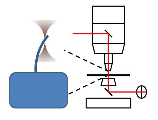
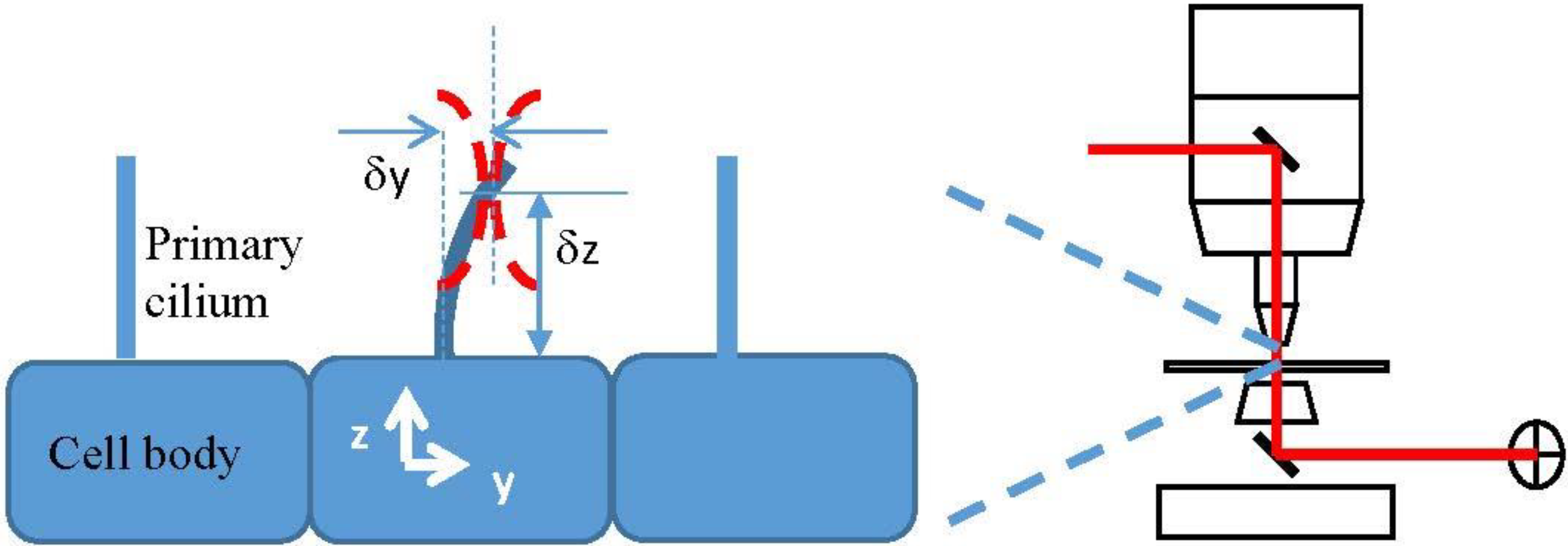
  • δx, δy, δz are the displacement of the center of the beam waist from the coordinate origin, which we place at the center of the base of the cilium.
For the numerical calculations performed here, P = 0.5 W, NA = 0.95, and λ0 = 1.064 µm, corresponding to our experimental apparatus. The culture media is an aqueous saline solution with estimated refractive index nm =1.33, resulting in z0 = 1.2 μm and ω0 = 0.32 μm. When appropriate, we set the refractive index of the cilium nc = 1.35, based on the chemical composition of the cilium [6].
Similarly, for numerical calculations presented here, we set the length of a cilium h = 3 µm and diameter d = 0.2 µm. The length of the cilium is regulated by the cell in response to stimulation by flow [6] or other biochemical factors (for example, [32]), and 3 μm is a typical length.
We note that in this paper, Equation (2) models the focused laser beam using the paraxial approximation even though our microscope objective is specified as sin(θ) = 0.71, corresponding to an error of 12% as compared to sin(θ) = θ. Incorporating higher-order corrections, for example [33] or using vectorial diffraction theory [34] is beyond the scope of this paper.

2. Results

2.1. The Force on a Dipole and the Force Density

In Appendix A and Figure 2 it is shown that for our experimental conditions the fraction of the electric field produced by neighboring dipoles provides a negligible contribution to the total field, greatly simplifying the analysis. Ignoring the scattered field contributions, the force on an individual dipole can be calculated using F ( r i ) =   α 2 i ( E i b e a m * E i b e a m ) .
Figure 2. (a) A plot of the points in a discretized cilium; (b) A plot of the ratio of the scattered electric field in the y direction from the other dipoles to the total electric field in the y direction as a function of s (microns) along the length of the cilium for (δx, δy, δz) = (0 µm, 0 µm, 1.5 µm). Notice that the field from the other dipoles is never more than 3/100 of the total field.
Photonics 02 00604 g002
For the y-polarized beam F ( r i ) = F ( r i ) y ^ :
F ( r i ) = 2 α E 0 2 ω 0 2 ω i 4 ( y i δ y ) e x p ( 2 ρ i 2 / ω i 2 )
Extending this result by passing from discrete dipoles to a continuous distribution suggests a force density ‘f’ in the y direction of the form
f ( r ) = 2 α E 0 2 ω 0 2 ω ( z ) 4 ( y δ y ) e x p ( 2 ρ ( x , y ) 2 / ω ( z ) 2 )
Modeling the cilium as a circular cylinder of diameter ‘d’ and height ‘h’ with base centered at the origin and axoneme oriented in the z direction, the total force in the y direction is given by
F = 0 h d / 2 d / 2 ( d / 2 ) 2 y 2 ( d / 2 ) 2 y 2 f ( r ) d x d y d z

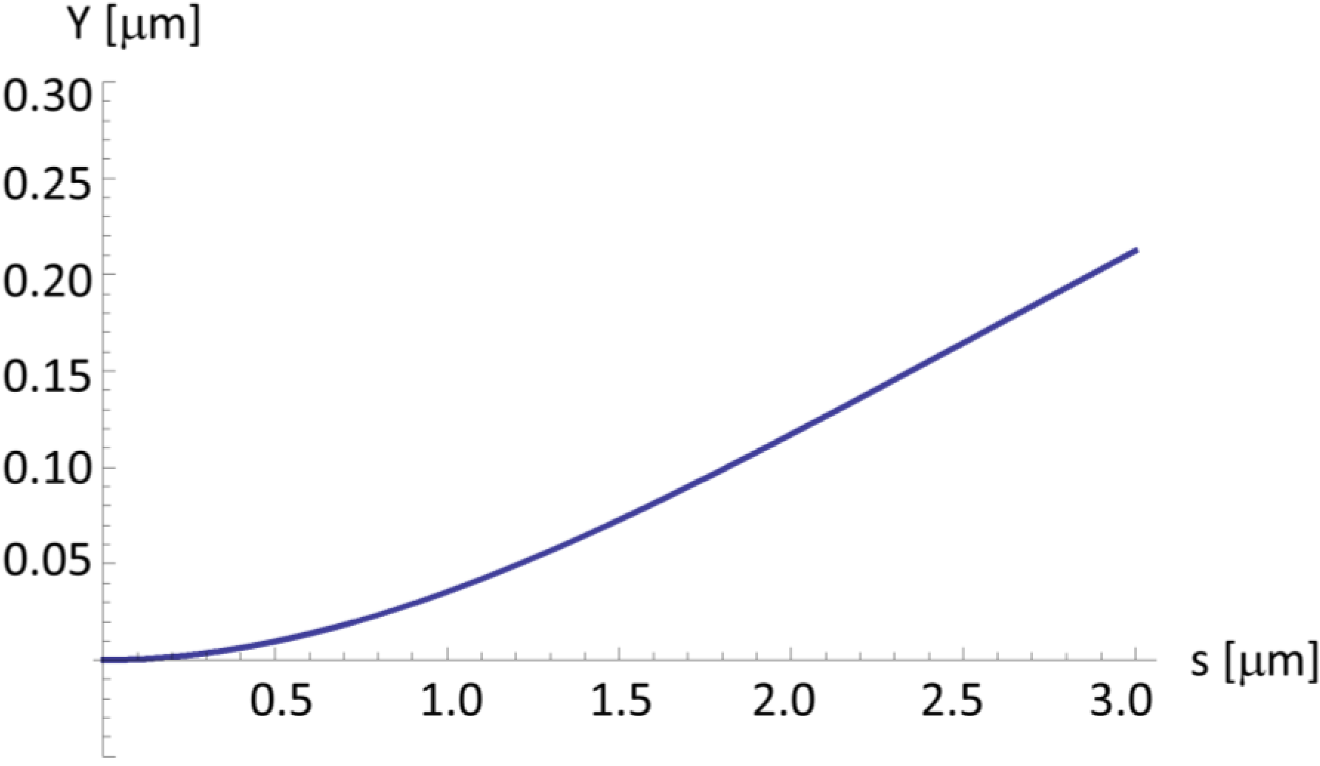
2.2. The z Dependence of the Force Density and the Bending of a Cilium

Here we use time-independent Euler–Bernoulli beam theory [35], valid for small static deformations of beams under constant load. The load on the cilium at a particular value of ‘z’ is given by integrating the force density over the cross section of the cilium at that value of ‘z’.
The displacement of the centerline of the cilium in the y direction (‘Y’) at any position along its length, parameterized by ‘s’, is given by solving the differential equation:
E I d 4 Y d s 4 = F ( s ) =   f ( s ) d A ( s ) = [ d 2 + Y ( s ) ] d 2 + Y ( s ) ( d / 2 ) 2 [ y Y ( s ) ] 2 ( d / 2 ) 2 [ y Y ( s ) ] 2 f d x d y
where E is the elastic modulus (the mechanical property we wish to measure), I is the second moment of area of a cross section of the cilium I = πd4, and boundary conditions Y(0) = 0, Y'(0) = 0, Y''(h) = 0, and Y'''(h) = 0. These boundary conditions correspond to a “simply supported” beam with “free end”. Extension to the time-dependent problem (say, for oscillatory or pulsatile applied flow occurring in vivo) is straightforward but not relevant for this report. In Equation (6), we modeled the cilium as a stack of infinitesimally-thin disks of diameter ‘d’, each laterally displaced by an amount Y(s). The coordinate s is related to z by ds2 = dz2 + dY2. For small deformations, s ≈ z. When appropriate, we set E = 1.2 * 10‑8N * μm−2 based on published reports [5,17,36,37,38].

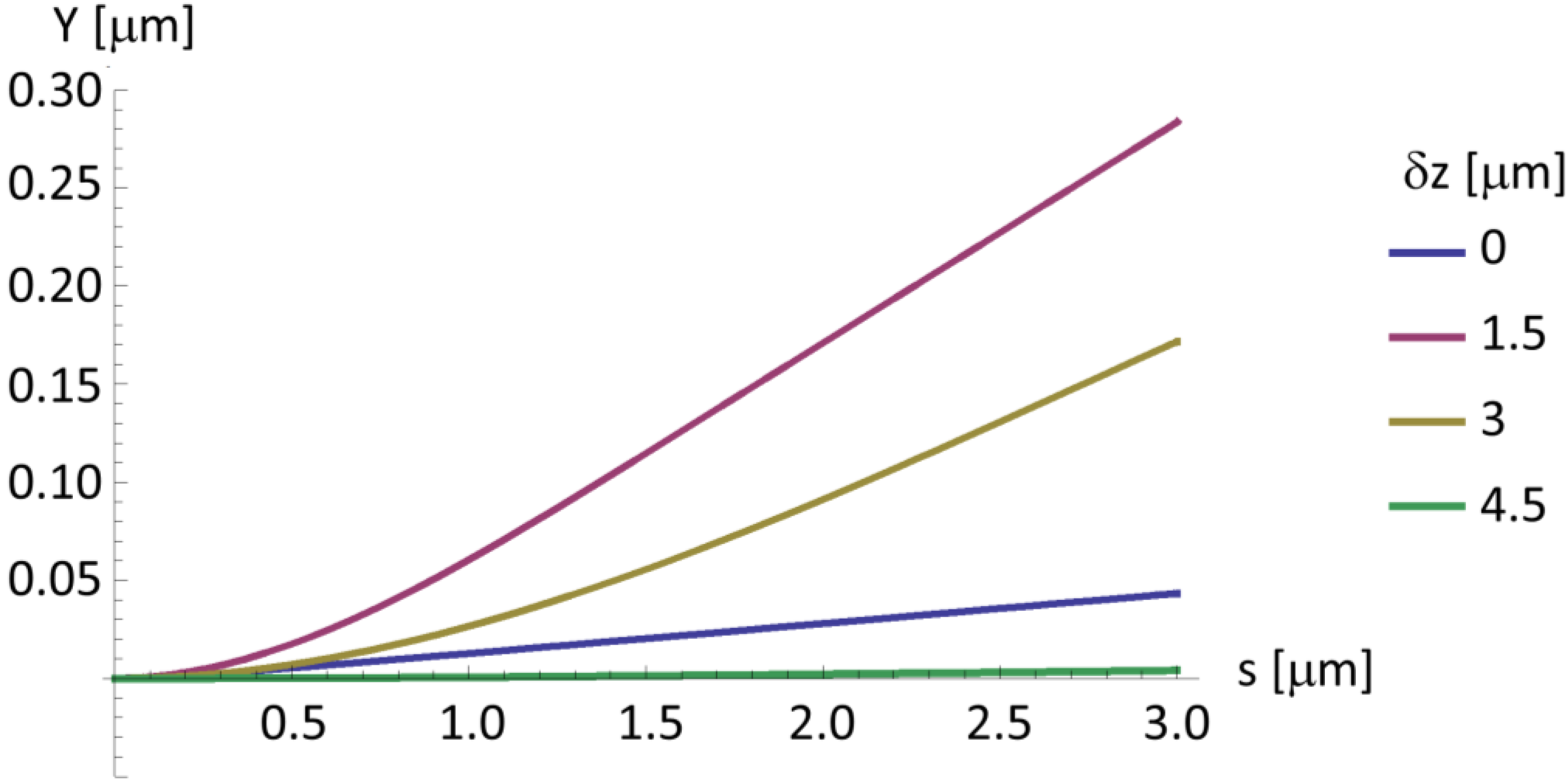
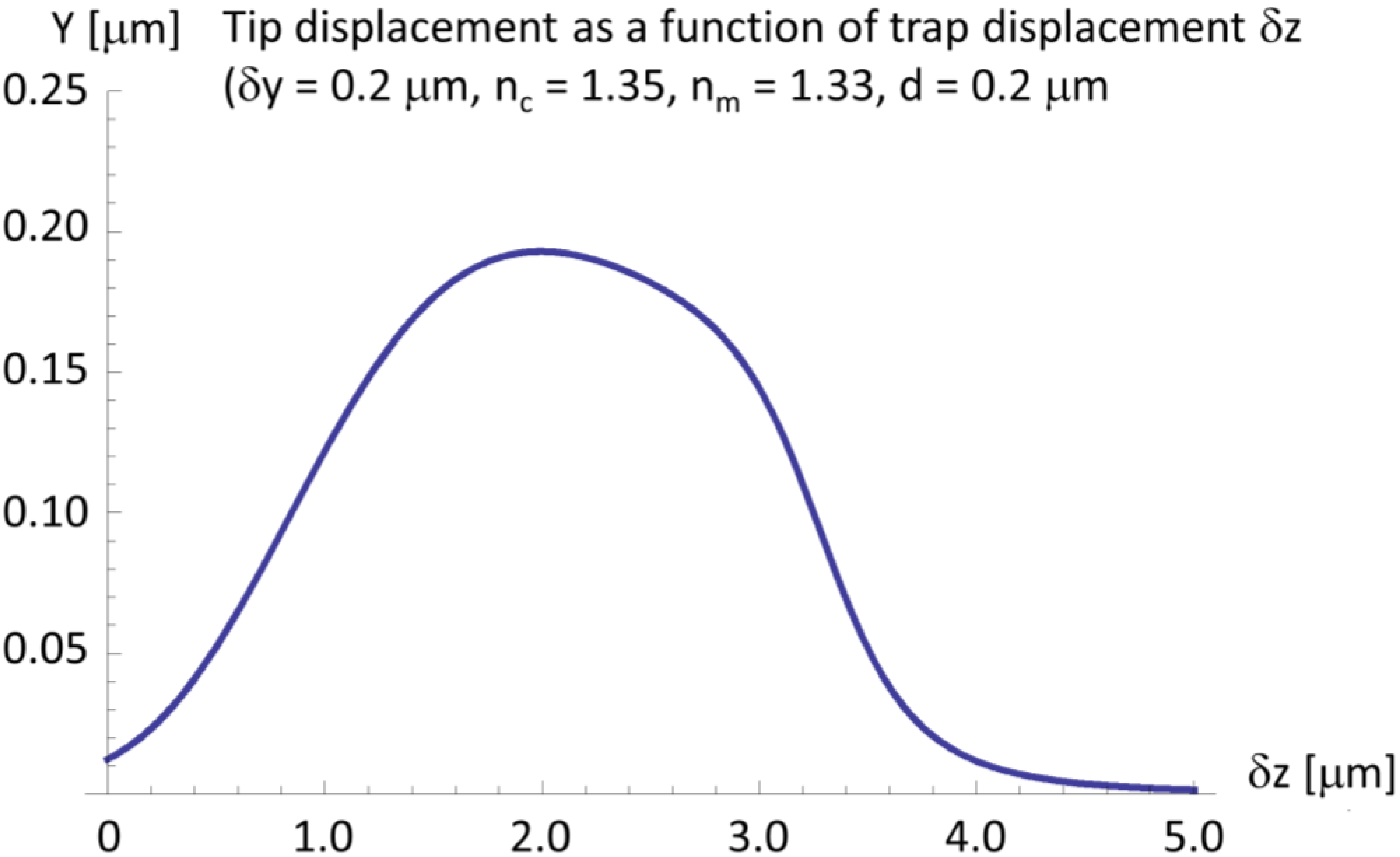
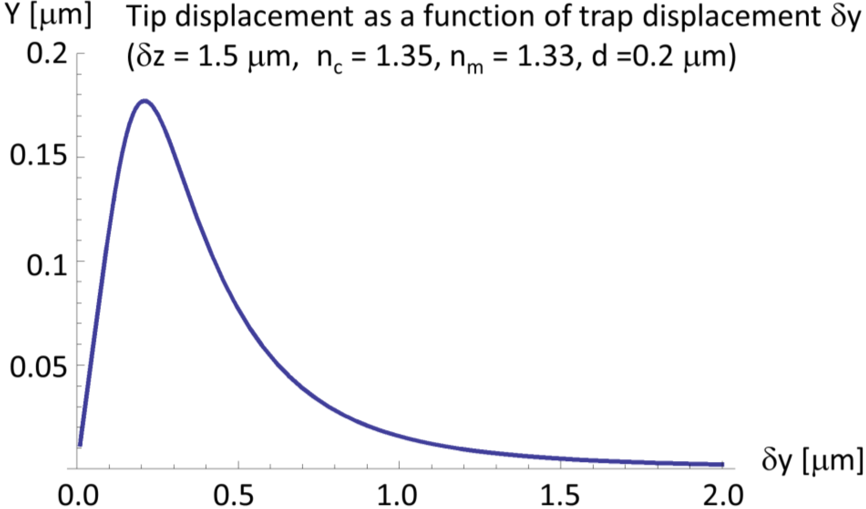
2.3. The General Case

Equation (6) is not, in general, analytically solvable. Instead, we used an approximate analytic solution using series representations, giving:
f ( s ) d A 6 ϵ m ϵ 0 ϵ c ϵ m ϵ c + 2 ϵ m ω 0 2 E 0 2 × j = 0 k = 0 l = 0 2 k + 1 m = 0 p = 0 2 j q = 0 2 m r = 0 8 ( 1 ) j + k + m + p + q π j ! k ! ( 2 k + 1 ) ( 2 j + 2 m p q + 1 )   × ( 2 ω ( z ) 2 ) j + k + 1 ( d 2 ) 2 k + 2 j + m l p q r + 3 ( 2 k + 1 l ) ( k + 1 2 l 2 m ) ( 2 j p ) ( 2 m q ) × ( 2 j + 2 m p q + 1 r ) ( δ y ) p Y q + r ( δ x ) l
Appendix B derives this result, using the assumption that the beam is only displaced from the origin in the direction of polarization and z. Although Equation (7) is rather complex, it does converge rapidly, as shown in Figure 3.
Figure 3. Plots of Equation (7) with increasing numbers of terms, indicated on the plot. The series converges rapidly, indicating that only the first 5 or 10 terms are required for numerical evaluation.
Photonics 02 00604 g003
Using the series approximation, Equation (6) can be numerically solved, providing a final equilibrium deformed shape of the cilium. The model can also output other experimentally convenient parameters, for example the displacement of the cilium tip from equilibrium.
Example plots of Equation (7) are shown for a representative experiment (Figure 4), allowing the displacement of the center of the trap relative to the cilium base to vary (Figure 5, Figure 6 and Figure 7) and allowing the bending stiffness to vary (Figure 8).
Figure 4. Example deformation of a primary cilium for a representative experiment. The trap parameters: incident power P = 0.5 W, trapping lens numerical aperture NA = 0.95, and trap wavelength λ0 = 1.064 µm. The trap center was displaced from the cilium base by δy = 0.2 µm and δz = 2.5 µm. The cilium length is 3.0 µm.
Photonics 02 00604 g004
Figure 5. Example deformation of a primary cilium for a representative experiment, showing the effect of allowing the vertical displacement of the trap from the cilium base δz = 0, 1.5, 3, and 4.5 µm. The trap parameters: incident power P = 0.5 W, trapping lens numerical aperture NA = 0.95, and trap wavelength λ0 = 1.064 µm. The trap center was displaced from the cilium axis by δy = 0.2 µm. The cilium length is 3.0 µm.
Photonics 02 00604 g005
Figure 6. Example deformation of a primary cilium for a representative experiment, showing the effect of varying the vertical displacement of the trap from the cilium base δz. Data graphs the displacement of the cilium tip Y(3) as δz is varied. The trap parameters: incident power P = 0.5 W, trapping lens numerical aperture NA = 0.95, and trap wavelength λ0 = 1.064 µm. The trap center was displaced from the cilium axis by δy = 0.2 µm. The cilium length is 3.0 µm.
Photonics 02 00604 g006
Figure 7. Example deformation of a primary cilium for a representative experiment, showing the effect of varying the horizontal displacement of the trap from the cilium axis δy. Data graphs the displacement of the cilium tip Y(3). The trap parameters: incident power P = 0.5 W, trapping lens numerical aperture NA = 0.95, and trap wavelength λ0 = 1.064 µm. The trap center was displaced from the cilium axis by δz = 1.5 µm. The cilium length is 3.0 µm.
Photonics 02 00604 g007
Figure 8. Example deformation of a primary cilium for a representative experiment, showing the effect of varying the bending modulus of the primary cilium. Data graphs the displacement of the cilium tip Y(3). The trap parameters: incident power P = 0.5W, trapping lens numerical aperture NA = 0.95, and trap wavelength λ0 = 1.064 µm. The trap center was displaced from the cilium axis by δy = 0.5 µm and δz = 1.5 µm. The cilium length is 3.0 µm.
Photonics 02 00604 g008

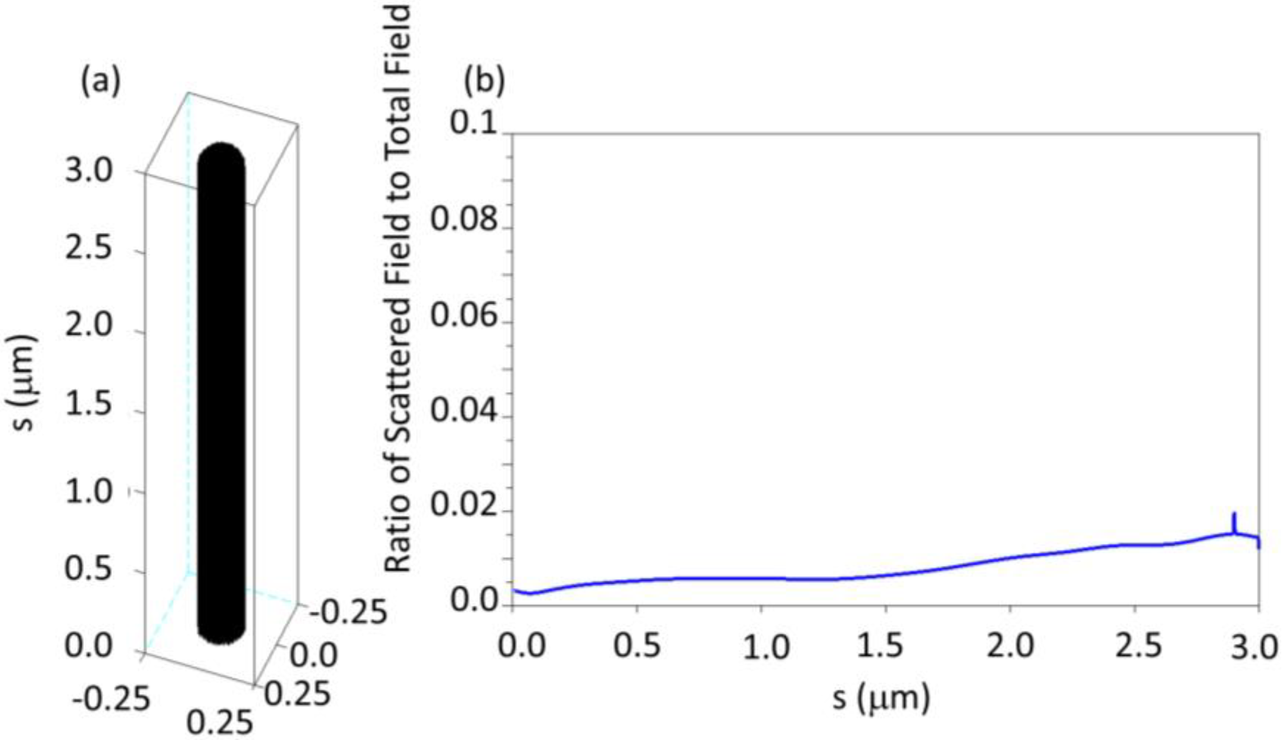
2.4. A Very Narrow Cylinder

An alternative to the complicated approximation of the load from Equation (7) is to treat the cilium as a one-dimensional object, one dipole thick. This changes the polarizability to
α = 3 ϵ m ϵ 0 π ( d 2 ) 2 ϵ c ϵ m ϵ c + 2 ϵ m δ ( ρ )
Passing to a continuous medium, the differential equation describing the deformation of the cilium is
d 4 Y d z 4 6 P E c π 2 d 2 ω 4 n c 2 n m 2 n c 2 + 2 n m 2 ( δ y Y ) e x p ( 2 ( δ y Y ) 2 / ω 2 )
where Y is the position of the center of the cilium. Figure 9 compares the results from Equations (7) and (9), showing that the 1-D approximation provides reasonable results as compared to the full 3-D expression.
Figure 9. Example deformation of a primary cilium for a representative experiment, showing the effect of idealizing the primary cilium as a 1-D object. Finite cilium diameter (red), the 1-D idealized approximation (blue). The trap parameters: incident power P = 0.5 W, trapping lens numerical aperture NA = 0.95, and trap wavelength λ0 = 1.064 µm. The trap center was displaced from the cilium axis by δy = 0.5 µm and δz = 1.5 µm. The cilium length is 3.0 µm.
Photonics 02 00604 g009

3. Discussion

There are two aspects to our results presented above. First, we have demonstrated a method to calculate the applied force by an optical trap. We have shown that our model can output a variety of measurable results (cilium profile, tip displacement) as a function of several different experimental inputs (trap displacement, cilium mechanical properties). For example, in concert with measured data, we can determine the bending modulus of a primary cilium.
The rationale for using optical trapping to stimulate a primary cilium rather than fluid flow is that optical traps apply a precise force to a single cilium, rather than apply a force to the entire apical surface of cells. Thus, optical trapping has specific advantages as a tool to study ciliary mechanosensation. Since quantitative knowledge of the applied force is essential to use optical trapping in this context, our results provide justification and validation of our optical trap method.

4. Conclusions

The motivation for this work was to develop a method to accurately measure the mechanical properties of the primary cilium. Laser tweezers offers the ability to apply a quantified force in a non-contact fashion. The goal here was to develop an initial model that can be used to analyze experimental data (total applied force, movement of the cilium tip) that we can obtain in the laboratory. The approximations introduced here were motivated by complexity of the analytical expression. Thus, we took pains to demonstrate that our approximate solution still provides results with sufficient accuracy and precision to be useful. However, it may be necessary to use more complicated differential equations to find the final deformation when accounting for environmental factors such as fluid flow, gravity, and thermal fluctuations. Similarly, solving the dynamic Euler-Bernoulli equation for beam oscillation may introduce additional complicating factors that we have not yet accounted for. For example, as the cilium is bending, the integrals in Equation (4) and (6) will depend on time. It is possible that a modified shooting approach [39] could be used, but a fully dynamic model is beyond the scope of this paper.
The final deformation profile of the cilium is a function of many variables. Importantly, one of them is the elastic modulus, a measure of stiffness. By measuring the displacement of the tip of the cilium for many different positions of the center of the optical trap it should be possible to infer the value of the bending modulus and the refractive index. It is critical to note that our model allows us to determine the mechanical properties of the primary cilium by only measuring the tip displacement. This is significant because the geometry of the primary cilium (parallel to the optical axis) greatly complicates attempts to image the entire axoneme. Thus, our model has a significant advantage because a single measurement of the tip displacement is sufficient to constrain the model and determine, for example, the bending modulus. Accurately characterizing the mechanical properties of the primary cilium is an essential step in demonstrating the biological relevance of this organelle.

Acknowledgments

The research was supported by the NIH DK092716 award.

Author Contributions

Both authors affirm that they equally contributed to this manuscript: obtaining and generating results, writing and editing, and generation of figures.

Appendix A: Using the DDA to Calculate the Scattered Electric Field

Starting from Equation (1) and substituting
G ( r i , r j ) p ( r j ) =   e x p ( i k r i j ) 4 π ϵ 0 r i j 3 [ k 2 r i j × ( r i j × p ( r j ) ) + 1 i k r i j r i j 2 ( r i j 2 p ( r j ) 3 r i j ( r i j p ( r j ) ) ) ]
for the scattered field contributions from other dipoles gives the local electric field
E ( r i ) E b e a m ( r i ) + α j i e x p ( i k r i j ) 4 π ϵ 0 r i j 3 [ k 2 ( ( r i j E b e a m ( r j ) ) r i j r i j 2 E b e a m ( r j ) ) + 1 i k r i j r i j 2 ( r i j 2 E b e a m ( r j ) 3 r i j ( r i j E b e a m ( r j ) ) ) ]
where r i j = r i r j and r i j = | r i j | . Since the relative polarizability is small, terms of second order dependence or higher are neglected.
The cilium is modeled as a cylinder with a hemispherical top shown in Figure 2. SciLab 5.3.3 code was written to evaluate the above expressions. Our results show that the scattered field in the y direction is very small compared to the total electric field in the y direction. Therefore, the scattered field can be ignored for our purposes.

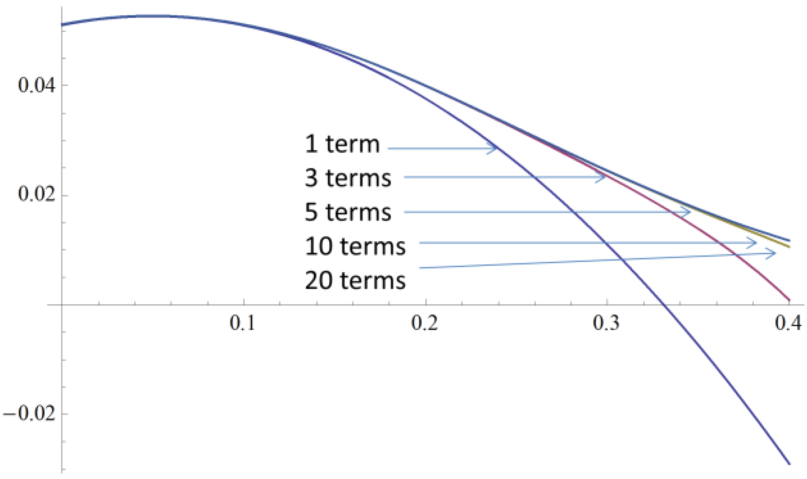
Appendix B: Series Solution for the Force on a Cylinder

The goal is to evaluate the integral:
f ( s ) d A = K [ d 2 + Y ] d 2 + Y ( d / 2 ) 2 [ y Y ] 2 ( d / 2 ) 2 [ y Y ] 2 ( y δ y ) e x p ( 2 ω ( z ) 2 [ ( y δ y ) 2 + ( x δ x ) 2 ] ) d x d y
Using the error function π 2 E r f ( x ) = exp ( x 2 ) d x , we first obtain
( d / 2 ) 2 [ y Y ] 2 ( d / 2 ) 2 [ y Y ] 2 e x p ( 2 ω ( z ) 2 [ ( y δ y ) 2 + ( x δ x ) 2 ] ) d x = ω ( z ) π 2 2 exp [ 2 ( ( y δ y ) ω ( z ) ) 2 ] [ E r f ( 2 ( ( d / 2 ) 2 [ y Y ] 2 δ x ) ω ( z ) ) + E r f ( 2 ( ( d / 2 ) 2 [ y Y ] 2 + δ x ) ω ( z ) ) ]
Using the following series expansions:
π 2 E r f ( a + x ) = k = 0 ( 1 ) k ( a + x ) 2 k + 1 k ! ( 2 k + 1 )
( x ± y ) n = k = 0 n ( n k ) x n k ( ± y ) k = k = 0 n n ! k ! ( n k ) ! x n k ( ± y ) k
( y δ y ) e x p [ 2 ω ( z ) 2 ( y δ y ) 2 ] = k = 0 ( 2 ω ( z ) 2 ) k ( y δ y ) 2 k + 1 k !
To first obtain
E r f 2 ( ( d / 2 ) 2 [ y Y ] 2 δ x ) ω ( z ) + E r f 2 ( ( d / 2 ) 2 [ y Y ] 2 + δ x ) ω ( z ) = k = 0 l = 0 2 k + 1 m = 0 2 ( 1 ) k π k ! ( 2 k + 1 ) ( 2 ω ( z ) ) 2 k + 1 ( 2 k + 1 l ) ( k + 1 2 l 2 m ) ( 1 ) m ( y Y ) 2 m   × ( d 2 ) 2 k + 2 l m [ ( δ x ) l + ( δ x ) l ] = { k = 0 l = 0 2 k + 1 m = 0 4 ( 1 ) k + m π k ! ( 2 k + 1 ) ( 2 k + 1 l ) ( k + 1 2 l 2 m ) ( 2 ω ( z ) ) 2 k + 1   ( y Y ) 2 m   ×   ( d 2 ) 2 k + 2 l m ( δ x ) l , l   e v e n 0 ,   l   o d d
From here, we assume ‘l’ is even. Then,
exp [ 2 ( ( y δ y ) ω ( z ) ) 2 ] [ E r f ( 2 ( ( d / 2 ) 2 [ y Y ] 2 δ x ) ω ( z ) ) + E r f ( 2 ( ( d / 2 ) 2 [ y Y ] 2 + δ x ) ω ( z ) ) ] = j = 0 k = 0 l = 0 2 k + 1 m = 0 4 ( 1 ) j + k + m π k ! ( 2 k + 1 ) ( 2 ω ( z ) 2 ) j + k + 1 ( y δ y ) 2 j j ! ( 2 k + 1 l ) ( k + 1 2 l 2 m )   × ( y Y ) 2 m ( d 2 ) 2 k + 2 l m ( δ x ) l
And finally:
f ( s ) d A = K j = 0 k = 0 l = 0 2 k + 1 m = 0 p = 0 2 j q = 0 2 m 4 ( 1 ) j + k + m + p + q π j ! k ! ( 2 k + 1 ) ( 2 ω ( z ) 2 ) j + k + 1 ( d 2 ) 2 k + 2 l m × ( 2 k + 1 l ) ( k + 1 2 l 2 m ) ( 2 j p ) ( 2 m q ) ( δ y ) p Y q ( δ x ) l [ d 2 + Y ] d 2 + Y y 2 j + 2 m p q d y = K j = 0 k = 0 l = 0 2 k + 1 m = 0 p = 0 2 j q = 0 2 m r = 0 8 ( 1 ) j + k + m + p + q π j ! k ! ( 2 k + 1 ) ( 2 j + 2 m p q + 1 ) ( 2 ω ( z ) 2 ) j + k + 1 × ( d 2 ) 2 k + 2 j + m l p q r + 3 × ( 2 k + 1 l ) ( k + 1 2 l 2 m ) ( 2 j p ) ( 2 m q ) ( 2 j + 2 m p q + 1 r ) ( δ y ) p Y q + r ( δ x ) l
where 2j + 2m-p-q is even.
This expression is considerably simplified with the approximation d → 0; for a Gaussian beam displaced from the cilium axis a distance ‘δρ’,
F ( z ) = 6 ϵ m ϵ 0 ϵ c ϵ m ϵ c + 2 ϵ m E 0 2 ω 0 2 ω ( z ) 4 ( δρ ) e x p ( 2 ( δρ ) 2 / ω ( z ) 2 )
when δx or δy = 0; this sum is equal to 0 and, therefore, the applied force when the trap is centered on the cilium axis is equal to 0.

Conflict of Interest

The authors declare no conflict of interest.

References

  1. Praetorius, H.A.; Spring, K.R. The renal cell primary cilium functions as a flow sensor. Curr. Opin. Nephrol. Hypertens 2003, 12, 517–520. [Google Scholar] [CrossRef] [PubMed]
  2. Miyoshi, K.; Kasahara, K.; Miyazaki, I.; Asanuma, M. Factors that influence primary cilium length. Acta Med. Okayama 2011, 65, 279–285. [Google Scholar] [PubMed]
  3. Rikmenspoel, R. Elastic properties of the sea urchin sperm flagellum. Biophysical journal 1966, 6, 471–479. [Google Scholar] [CrossRef]
  4. Baba, S.A. Flexural rigidity and elastic constant of cilia. J. Exp. Biol. 1972, 56, 459–467. [Google Scholar] [PubMed]
  5. Schwartz, E.A.; Leonard, M.L.; Bizios, R.; Bowser, S.S. Analysis and modeling of the primary cilium bending response to fluid shear. Am. J. Physiol. 1997, 272, F132–F138. [Google Scholar] [PubMed]
  6. Resnick, A.; Hopfer, U. Force-response considerations in ciliary mechanosensation. Biophys. J. 2007, 93, 1380–1390. [Google Scholar] [CrossRef] [PubMed]
  7. Resnick, A.; Hopfer, U. Mechanical stimulation of primary cilia. Front. Biosci. 2008, 13, 1665–1680. [Google Scholar] [CrossRef] [PubMed]
  8. Mans, D.A.; Voest, E.E.; Giles, R.H. All along the watchtower: Is the cilium a tumor suppressor organelle? Biochim. Biophys. Acta 2008, 1786, 114–125. [Google Scholar] [PubMed]
  9. Jenkins, P.M.; McEwen, D.P.; Martens, J.R. Olfactory cilia: Linking sensory cilia function and human disease. Chem. Senses 2009, 34, 451–464. [Google Scholar] [CrossRef] [PubMed]
  10. Veland, I.R.; Awan, A.; Pedersen, L.B.; Yoder, B.K.; Christensen, S.T. Primary cilia and signaling pathways in mammalian development, health and disease. Nephron Physiol. 2009, 111, 39–53. [Google Scholar] [CrossRef] [PubMed]
  11. Peterson, M.A. Geometry of ciliary dynamics. Phys. Rev. E Stat. Nonlinear Soft Matter Phys. 2009, 80, 011923. [Google Scholar] [CrossRef]
  12. Kim, S.; Dynlacht, B.D. Assembling a primary cilium. Curr. Opin. Cell Biol. 2013, 25, 506–511. [Google Scholar] [CrossRef] [PubMed]
  13. Fisch, C.; Dupuis-Williams, P. Ultrastructure of cilia and flagella—Back to the future! Biol. Cell 2011, 103, 249–270. [Google Scholar] [CrossRef] [PubMed]
  14. Pozrikidis, C. Shear flow past slender elastic rods attached to a plane. Int. J. Solids Struct. 2011, 48, 137–143. [Google Scholar] [CrossRef]
  15. Eloy, C.; Lauga, E. Kinematics of the most efficient cilium. Phys. Rev. Lett. 2012, 109, 038101. [Google Scholar] [CrossRef] [PubMed]
  16. Hilfinger, A.; Chattopadhyay, A.K.; Julicher, F. Nonlinear dynamics of cilia and flagella. Phys. Rev. E Stat. Nonlinear Soft Matter Phys. 2009, 79, 051918. [Google Scholar] [CrossRef]
  17. Young, Y.N.; Downs, M.; Jacobs, C.R. Dynamics of the primary cilium in shear flow. Biophys. J. 2012, 103, 629–639. [Google Scholar] [CrossRef] [PubMed]
  18. Battle, C. Mechanics & Dynamics of the Primary Cilium; Georg-August-Universität Göttingen: Göttingen, Germany, 2013. [Google Scholar]
  19. Ashkin, A. Acceleration and trapping of particles by radiation pressure. Phys. Rev. Lett. 1970, 24, 156. [Google Scholar] [CrossRef]
  20. Ashkin, A.; Dziedzic, J.M.; Bjorkholm, J.E.; Chu, S. Observation of a single-beam gradient force optical trap for dielectric particles. Opt. Lett. 1986, 11, 288–290. [Google Scholar] [CrossRef] [PubMed]
  21. Felgner, H.; Frank, R.; Schliwa, M. Flexural rigidity of microtubules measured with the use of optical tweezers. J. Cell Sci. 1996, 109, 509–516. [Google Scholar] [PubMed]
  22. Wiggins, C.H.; Riveline, D.; Ott, A.; Goldstein, R.E. Trapping and wiggling: Elastohydrodynamics of driven microfilaments. Biophys. J. 1998, 74, 1043–1060. [Google Scholar] [CrossRef]
  23. Glaser, J.; Hoeprich, D.; Resnick, A. Near real-time measurement of forces applied by an optical trap to a rigid cylindrical object. Opt. Eng. 2014, 53. [Google Scholar] [CrossRef]
  24. Ren, K.F.; Grehan, G.; Gouesbet, G. Scattering of a gaussian beam by an infinite cylinder in the framework of generalized lorenz-mie theory: Formulation and numerical results. J. Opt. Soc. Am. A 1997, 14, 3014–3025. [Google Scholar] [CrossRef]
  25. Kozaki, S. Scattering of a gaussian-beam by an inhomogeneous dielectric cylinder. J. Opt. Soc. Am. 1982, 72, 1470–1474. [Google Scholar] [CrossRef]
  26. Lock, J.A. Scattering of a diagonally incident focused gaussian beam by an infinitely long homogeneous circular cylinder. J. Opt. Soc. Am. A 1997, 14, 640–652. [Google Scholar]
  27. Ling, L.; Zhou, F.; Huang, L.; Li, Z.Y. Optical forces on arbitrary shaped particles in optical tweezers. J. Appl. Phys. 2010, 108. [Google Scholar] [CrossRef]
  28. Simpson, S.H.; Hanna, S. Application of the discrete dipole approximation to optical trapping calculations of inhomogeneous and anisotropic particles. Opt. Express 2011, 19, 16526–16541. [Google Scholar] [CrossRef] [PubMed]
  29. Yurkin, M.A.; Hoekstra, A.G.; Brock, R.S.; Lu, J.Q. Systematic comparison of the discrete dipole approximation and the finite difference time domain method for large dielectric scatterers. Opt. Express 2007, 15, 17902–17911. [Google Scholar] [CrossRef] [PubMed]
  30. Jia, L.; Thomas, E.L. Optical forces and optical torques on various materials arising from optical lattices in the lorentz-mie regime. Phys. Rev. B 2011, 84. [Google Scholar] [CrossRef]
  31. Wriedt, T. A review of elastic light scattering theories. Part. Part. Syst. Char. 1998, 15, 67–74. [Google Scholar] [CrossRef]
  32. Verghese, E.; Zhuang, J.; Saiti, D.; Ricardo, S.D.; Deane, J.A. In vitro investigation of renal epithelial injury suggests that primary cilium length is regulated by hypoxia-inducible mechanisms. Cell Biol. Int. 2011, 35, 909–913. [Google Scholar] [CrossRef] [PubMed]
  33. Barton, J.P.; Alexander, D.R. 5th-order corrected electromagnetic-field components for a fundamental gaussian-beam. J. Appl. Phys. 1989, 66, 2800–2802. [Google Scholar] [CrossRef]
  34. Gu, M. Advanced Optical Imaging Theory; Springer: Berlin, Germany; New York, NY, USA, 2000; p. 214. [Google Scholar]
  35. Segel, L.A.; Handelman, G.H. Mathematics Applied to Continuum Mechanics; Society for Industrial and Applied Mathematics: Philadelphia, PA, USA, 2007; p. 590. [Google Scholar]
  36. Downs, M.E.; Nguyen, A.M.; Herzog, F.A.; Hoey, D.A.; Jacobs, C.R. An experimental and computational analysis of primary cilia deflection under fluid flow. Comput. Methods Biomech. Biomed. Eng. 2014, 17, 2–10. [Google Scholar] [CrossRef] [PubMed]
  37. Han, Y.F.; Ganatos, P.; Weinbaum, S. Transmission of steady and oscillatory fluid shear stress across epithelial and endothelial surface structures. Phys. Fluids 2005. [Google Scholar] [CrossRef]
  38. Liu, W.; Xu, S.; Woda, C.; Kim, P.; Weinbaum, S.; Satlin, L.M. Effect of flow and stretch on the [ca2+]i response of principal and intercalated cells in cortical collecting duct. Am. J. Physiol. 2003, 285, F998–F1012. [Google Scholar]
  39. Ibrahim, S.M.; Patel, B.P.; Nath, Y. Modified shooting approach to the non-linear periodic forced response of isotropic/composite curved beams. Int. J. Nonlinear Mech. 2009, 44, 1073–1084. [Google Scholar] [CrossRef]

