Fault Detection in Wastewater Treatment Systems Using Multiparametric Programming

Abstract

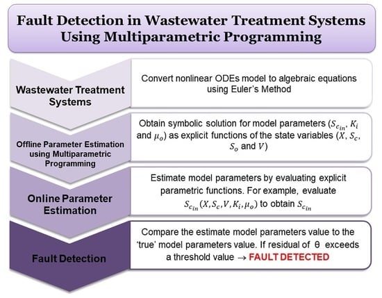
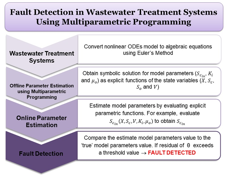
In this work, a methodology for fault detection in wastewater treatment systems, based on parameter estimation, using multiparametric programming is presented. The main idea is to detect faults by estimating model parameters, and monitoring the changes in residuals of model parameters. In the proposed methodology, a nonlinear dynamic model of wastewater treatment was discretized to algebraic equations using Euler’s method. A parameter estimation problem was then formulated and transformed into a square system of parametric nonlinear algebraic equations by writing the optimality conditions. The parametric nonlinear algebraic equations were then solved symbolically to obtain the concentration of substrate in the inflow, $S_{c_{in}}$, inhibition coefficient, $K_i$, and specific growth rate, ${\mu }_o$, as an explicit function of state variables (concentration of biomass, $X$; concentration of organic matter, $S_c$; concentration of dissolved oxygen, $S_o$; and volume, $V$). The estimated model parameter values were compared with values from the normal operation. If the residual of model parameters exceeds a certain threshold value, a fault is detected. The application demonstrates the viability of the approach, and highlights its ability to detect faults in wastewater treatment systems by providing quick and accurate parameter estimates using the evaluation of explicit parametric functions.

1. Introduction

Traditionally, wastewater treatment is a process of converting wastewater into bilge water that can be returned to the environment, and used for domestic and industrial applications. Nowadays, wastewater treatment plants (WWTPs) also focus on sustainability issues through recovery of energy and nutrients from wastewater [1,2,3]. With the increasing number of WWTPs worldwide, and the increasingly stricter requirements for maintaining the quality of effluents, on-line process monitoring has become an important aspect for ensuring efficient operation and management of WWTPs [4]. It involves a process of detecting faults and diagnosing their causes and locations. This is achieved by continuously monitoring the systems to detect any abnormal conditions, and then, evaluating and diagnosing the conditions with faults [5,6,7].

Fault detection methods for sensor faults in wastewater treatment (WWT) systems have normally used data-based methods, such as neural networks (NN) and principal component analysis (PCA). The neural network model was presented in Maier and Dandy [8] to model a wastewater treatment system. In Caccavale et al.’s work [9], faults in nitrogen sensors were detected by estimating the concentration of NO and NH using neural networks. Honggui et al. [10] showed how sensor faults can be diagnosed using the fuzzy neural network to estimate dissolved oxygen concentrations, pH, chemical oxygen demand (COD), and total nutrients. In Lee et al. [11], the kernel PCA was used to extract nonlinear relations in process variables, and it showed a better performance than linear PCA in process monitoring. Adaptive PCA was used in Baggiani and Marsili-Libelli [12] to compare the current plant operation with an exact performance based on a reference data set and sensor outputs. In Sanchez-Fernández et al. [13], a distributed PCA was applied to detect faults by minimizing the communication cost between the blocks in WWTPs. The classical principal component analysis was presented using Benchmark Simulation Model No. 1 (BSM1) in Garcia-Alvarez et al. [14], Chen et al. [15], and Carlsson and Zambrano [16]. The combined use of PCA in data preprocessing and artificial neural networks has been presented in Gontarski et al. [17] to improve network performance. Besides that, fault detection in WWT has been discussed using an observer-based method in Fragkoulis et al. [18], where multiple actuators and sensors faults were detected.

In an aerobic WWT system, respiration rate is used as an indicator of biological activity for monitoring and control [19,20]. The respiration rate is affected by the initial condition of biomass, substrate concentration in the inflow, and extrinsic growth behavior of the biomass on inhibitory substrates. In Wimberger and Verde [19], a fault detection and isolation was performed by evaluating the detectability and isolability of analytical- and signal-based methodologies using information from applying the sensitivity theory. However, respiration rate depends on intermittent aeration patterns, and the calculation can only be evaluated during air-off periods [21,22,23]. In this work, we propose fault detection in the WWT system by detecting and monitoring the kinetic parameters of extrinsic growth behavior using multiparametric programming. The main idea is to detect faults by estimating model parameters and monitoring the residual of model parameters. In parameter estimation-based fault detection, faults can be associated with the specific parameters of the model. With this assumption, parameters of a system are estimated on-line repeatedly using well known parameter estimation methods. The presence of faults is indicated if there is a discrepancy between the values of estimated parameters and the ‘true’ parameters. An overview for fault detection using parameter estimation can be found in [24,25,26,27,28,29,30,31].

In our earlier work [32], the fault detection method based on parameter estimation by using multiparametric programming [33,34,35,36,37,38,39] was presented. In that work, nonlinear ordinary differential equations model was converted into algebraic equations using Euler’s method. Then, a square system of parametric nonlinear algebraic equations was obtained by formulating Karush-Kuhn-Tucker (KKT) optimality conditions. The model parameters were then obtained as an explicit function of the measurements by symbolically solving the equations representing KKT conditions. The estimated model parameters were compared with the normal operation for fault detection. If the residual of model parameters exceeds a certain threshold value, a fault is detected.

In this work, the concentration of substrate in the inflow, inhibition coefficient, and specific growth rate were treated as model parameters and obtained as an explicit function of the measurements using multiparametric programming, and monitored for fault detection and diagnosis.

The rest of this paper is organized as follows: Section 2 presents the parameter estimation algorithm using multiparametric programming, and in Section 3, the wastewater treatment process reaction phase model is introduced. This section also includes detailed formulation for obtaining model parameters as an explicit function of measurements to detect faults. Section 4 evaluates the feasibility of parameter estimation using multiparametric programming in fault-free and faulty scenarios. Concluding remarks are presented in Section 5.

2. Problem Statement and Solution Approach

Problem Definition

Consider the following parameter estimation problem [40]:

Problem 1.

$${\epsilon }_{FD}=\underset{\mathsf{\theta },\mathbf{x}(t)}{\min }{{\displaystyle \sum _{j\in J}{\displaystyle \sum _{i\in I}\left\{{\widehat{x}}_j(t_i)-x_j(t_i)\right\}}}}^2$$

(1)

subject to:

$$\frac{d{x}_j(t)}{dt}=f_j\left(\mathbf{x}(t),\mathbf{u}(t),\mathsf{\theta },t\right),j\in J$$

(2)

$$x_j(t=0)=x_j^0,j\in J$$

(3)

$$t\in [0,t_f]$$

(4)

where $x(t)$ represents the J-dimensional vector of state variables in the given ordinary differential equations (ODEs) system, ${\widehat{x}}_j(t_i)$ represents the measurements of the state variables at the time points $t_i$, $\mathbf{u}(t)$ represents the vector of control variables, and $\mathsf{\theta }$ is the vector of parameters. An occurrence of fault can be attributed to changes in model parameters, $\mathsf{\theta }$, from the nominal values. A key difficulty with this approach for fault detection is that it requires an online solution of problem 1 at regular time intervals, which is computationally demanding and prone to failure of the numerical solver for Problem 1. These limitations can be overcome using multiparametric programming (MPP) to estimate the model parameters, $\mathsf{\theta }$, as an explicit function of measurements, ${\widehat{x}}_j(t_i)$, by treating $\mathsf{\theta }$ as optimization variables and ${\widehat{x}}_j(t_i)$ as the parameters. The algorithm for parameter estimation using MPP to obtain a symbolic solution for model parameters is summarized as follows [32]:

(i)

The nonlinear ODEs model in Equation (2) was discretized using Euler’s method to algebraic equations on the interval, $t\in [0,t_f]$. The Euler’s method provides

$$x_j(i+1)=x_j(i)+\Delta t{f}_j\left(x(i),u(i),\mathsf{\theta }\right),i\in I,j\in J$$

(5)

where the step size is given by $\Delta t$.

(ii)

Fault detection problem was formulated as a nonlinear programming (NLP) problem as follows:

Problem 2.

$${\epsilon }_{MPP}=\underset{\mathsf{\theta },\mathbf{x}(i)}{\min }{{\displaystyle \sum _{j\in J}{\displaystyle \sum _{i\in I}\left\{{\widehat{x}}_j(i+1)-x_j(i+1)\right\}}}}^2$$

(6)

subject to:

$$h_j=x_j(i+1)-x_j(i)-\Delta t{f}_j\left(x(i),u(i),\mathsf{\theta }\right)=0,i\in I,j\in J$$

(7)

$$x_j(0)=x_j^0,j\in J$$

(8)

where $h_j$ is the set of nonlinear algebraic equations obtained by discretizing the ODEs given by Equation (5), and $I=\left\{0,1\right\}$ is considered in this work.

(iii)

For Problem 2, the Lagrangian function is given by

$$L=g+{\displaystyle \sum _{j\in J}{\lambda }_j{h}_j}$$

(9)

where

$$g={\displaystyle \sum _{j\in J}{\displaystyle \sum _{i\in I}{\left\{{\widehat{x}}_j(i+1)-x_j(i+1)\right\}}^2}}$$

(10)

$$h_j=x_j(i+1)-x_j(i)-\Delta t{f}_j\left(x(i),u(i),\mathsf{\theta }\right)=0,i\in I,j\in J$$

(11)

and ${\lambda }_j$ represents the Lagrange multipliers. The first-order Karush-Kuhn-Tucker (KKT) conditions are given by the equality constrains as follows

$${\nabla }_{\mathsf{\theta }}L={\nabla }_{\mathsf{\theta }}g+{\nabla }_{\mathsf{\theta }}{\displaystyle \sum {\lambda }_j{h}_j}=0,j\in J$$

(12)

$$h_j=0$$

(13)

(iv)

The equality constraints corresponding to the KKT conditions given by Equations (12) and (13) were solved symbolically to obtain Lagrange multipliers and model parameters, $\mathsf{\theta }\left(\widehat{x}\right)$, as an explicit function of measurements, $\widehat{x}$.

(v)

The solutions obtained in the previous step were examined and solutions with imaginary parts were ignored.

(vi)

The estimated model parameters, $\mathsf{\theta }$, were calculated using the measurements, $\widehat{x}$, by simple evaluation of $\mathsf{\theta }\left(\widehat{x}\right)$.

(vii)

Faults were diagnosed by monitoring residual changes in model parameters. Any significant difference between estimated and observed model parameters may be attributed to occurrence of a fault.

3. Wastewater Treatment System

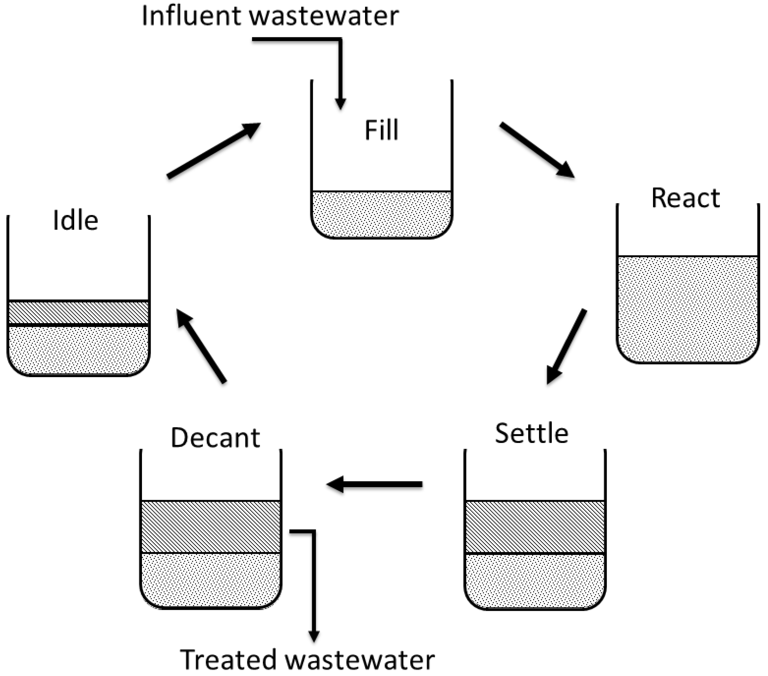
In this work, an aerobic sequencing batch reactor (SBR) model for fed-batch reactor operation mode was considered. The bioprocesses involved in the treatment used activated sludge and provided treatment for wastewater in five stages: Fill, react, settle, decant, and idle as shown in Figure 1 [41]. During the fill stage, the wastewater was directed into the tank and mixed with the sludge from previous cycles. At the reacting stage, air was provided as function of the aeration process that consumes the waste as nutrition and produces carbon dioxide, nitrates, and nitrites. After sufficient time of reaction, the aeration process was stopped and the sludge was allowed to settle. At the decant stage, the treated wastewater was removed from the reactor and the sludge that remained was reused for the next cycle. The reactor then entered the idle stage which was used to prepare the SBR for the next cycle.

The aerobic system involves aerobic growth and endogenous respiration reactions given by:

$$\mathrm{Growth}:S_c+S_o\to X$$

(14)

$$\mathrm{Endogenous}\mathrm{respiration}:S_c+X\to X$$

(15)

where $S_c$ represents the concentrations of organic matter, $S_o$ is the concentration of dissolved oxygen, and $X$ represents the concentration of biomass. The mathematical model of the process is given by the following equations [42]:

$$\frac{dX}{dt}=\mu X-\frac{q_{in}}{V}X$$

(16)

$$\frac{d{S}_c}{dt}=-k_1\mu X+\frac{q_{in}}{V}\left(S_{c_{in}}-S_c\right)$$

(17)

$$\frac{d{S}_o}{dt}=-k_2\mu X-bX+\frac{q_{in}}{V}\left(S_{o_{in}}-S_o\right)+k_{La}\left(S_{o_s}-S_o\right)$$

(18)

$$\frac{dV}{dt}=q_{in}$$

(19)

$$\mu =\frac{{\mu }_o{S}_c}{K_s+S_c+\frac{{S_c}^2}{K_i}}$$

(20)

where $\mu$ is specific growth rate, $q_{in}$ is inlet flow rate, $V$ is volume, $k_1$ and $k_2$ are yield coefficients, $b$ is endogenous respiration kinetic constant, $S_{c_{in}}$ is inlet organic matter, $S_{o_{in}}$ is dissolved oxygen concentrations, $k_{La}$ is transfer coefficient, and $S_{o_s}$ is oxygen saturation concentration. The specific growth rate, $\mu$, is represented by the Haldane model and is given by Equation (20). The parameter values for the wastewater treatment process reaction are shown in

Table 1. Model parameters for the wastewater treatment process.

Parameter	Value	Description
$S_{c_{in}}$	168 mg/L	the concentration of substrate in the inflow
$S_{o_{in}}$	0 mg/L	the concentration of dissolved oxygen in the inflow
$q_{in}$	14.8 mg/L	the inflow rate
$S_{o_s}$	6 mg/L	the dissolved oxygen mass at saturation
$k_1$	3.7	the conversion coefficient of the substrate to biomass
$k_2$	1.0363	the conversion coefficient of oxygen to biomass
$b$	0.0059 1/h	the endogenous respiration coefficient
$k_{La}$	16.8 1/h	the oxygen mass transfer coefficient
$K_i$	3.753 mg/L	the inhibition coefficient
$K_s$	60 mg/L	the half saturation coefficient
${\mu }_o$	0.1916 1/h	the specific growth rate

[19,42].

Fault Detection Problem for the Wastewater Treatment Process

In this work, a method to estimate and detect faults in wastewater treatment is presented. The concentration of substrate in the inflow, $S_{c_{in}}$, inhibition coefficient, $K_i$, and specific growth rate, ${\mu }_o$, were treated as model parameters and obtained as an explicit function of measurements using multiparametric programming and monitored for fault detection and diagnosis. By monitoring the estimated model parameters, process faults can be detected and diagnosed. We took this approach because the respiration rate indicates the biological activity, which is used for monitoring and control, and the respiration rate is affected by $S_{c_{in}}$, $K_i$, and ${\mu }_o$.

Thus, the objective of this fault detection problem is to estimate the model parameters, $S_{c_{in}}$, $K_i$, and ${\mu }_o$ by minimizing the error of parameter estimate, ${\epsilon }_{FD}$, between the measurement of state variables and model predicted value of state variables as shown in problem 3.

Problem 3.

$${\epsilon }_{FD}=\underset{S{c}_{in},K_i,{\mu }_o}{\min }{\displaystyle \sum _{i\in I}\{{(\widehat{X}(t_i)-X(t_i))}^2+{({\widehat{S}}_c(t_i)-S_c(t_i))}^2+{({\widehat{S}}_o(t_i)-S_o(t_i))}^2+{(\widehat{V}(t_i)-V(t_i))}^2\}}$$

(21)

subject to: Equations (16)–(20).

The formulation and solution of the parameter estimation problem using MPP for WWTP are presented as follow:

(i)

The nonlinear ODE model in Equations (16)–(19) is discretized using explicit Euler’s method and reformulated as the following algebraic equations:

$$X(i+1)=\Delta t(\frac{X(i)}{\Delta t}+\frac{S_c(i){\mu }_{o}X(i)}{K_s+S_c(i)+\frac{S_c{(i)}^2}{K_i}}-\frac{q_{in}}{V(i)})$$

(22)

$$S_c(i+1)=\Delta t(\frac{S_c(i)}{\Delta t}+\frac{q_{in}(-S_c(i)+S_{c_{in}})}{V(i)}-\frac{k_1{S}_c(i){\mu }_{o}X(i)}{K_s+S_c(k)+\frac{S_c{(i)}^2}{K_i}})$$

(23)

$$\begin{array}{ll}{S}_o(i+1)=& \Delta t(\frac{S_o(i)}{\Delta t}+k_{la}(-S_o(i)+S_{o_s})+\frac{q_{in}(-S_o(i)+S_{o_{in}})}{V(i)}-bX(i)-\\ & \frac{k_2{S}_c(i){\mu }_{o}X(i)}{K_s+S_c(i)+\frac{S_c{(i)}^2}{K_i}})\end{array}$$

(24)

$$V(i+1)=\Delta t{q}_{in}+V(i)$$

(25)

(ii)

The discrete-time fault detection problem is formulated as the following NLP:

Problem 4.

$$\begin{array}{ll}{\epsilon }_{MPP}=& \underset{S{c}_{in},K_i,{\mu }_o}{\min }{\displaystyle \sum _{i\in I}\{{(\widehat{X}(i+1)-X(i+1))}^2+{({\widehat{S}}_c(i+1)-S_c(i+1))}^2+}\\ & {({\widehat{S}}_o(i+1)-S_o(i+1))}^2+{(\widehat{V}(i+1)-V(i+1))}^2\}\end{array}$$

(26)

subject to:

$$\begin{array}{ll}{h}_1& =X(i+1)-X(i)-(\Delta t{S}_c(i){\mu }_{o}X(i))/(K_s+S_c(i)+(S_c{(i)}^2)/K_i)+\\ & (\Delta t{q}_{in})/V(i)\\ & =0\end{array}$$

(27)

$$\begin{array}{ll}{h}_2& =S_c(i+1)-\Delta t(S_c(i)-(\Delta t{q}_{in}(-S_c(i)+S_{c_{in}}))/V(i))+(\Delta t{k}_1{S}_c(i){\mu }_{o}X(i))/\\ & (K_s+S_c(i)+S_c{(i)}^2/K_i)\\ & =0\end{array}$$

(28)

$$\begin{array}{ll}{h}_3& =S_o(i+1)-S_o(i)-\Delta t{k}_{la}(-S_o(i)+S_{o_s})-(\Delta t{q}_{in}(-S_o(i)+S_{o_{in}}))/V(i)+\Delta tbX(i)+\\ & (\Delta t{k}_2{S}_c(i){\mu }_{o}X(i))/(K_s+S_c(i)+S_c{(i)}^2/K_i)\\ & =0\end{array}$$

(29)

$$h_4=V(i+1)-\Delta t{q}_{in}-V(i)=0$$

(30)

$$X(i)=X^0$$

(31)

$$S_c(i)={S_c}^0$$

(32)

$$S_o(i)={S_o}^0$$

(33)

$$V(i)=V^0$$

(34)

(iii)

Equations (27)–(30) are substituted into Equation (26) to obtain:

$$\begin{array}{ll}g& =(\widehat{X}(i+1)-(X(i)+(\Delta t{S}_c(i){\mu }_{o}X(i))/(K_s+S_c(i)+(S_c{(i)}^2)/K_i)-\\ & (\Delta t{q}_{in})/V(i)){)}^2+({\widehat{S}}_c(i+1)-(\Delta t(S_c(i)+(\Delta t{q}_{in}(-S_c(i)+S_{c_{in}}))/V(i))-\\ & (\Delta t{k}_1{S}_c(i){\mu }_{o}X(i))/(K_s+S_c(i)+S_c{(i)}^2/K_i)){)}^2+({\widehat{S}}_o(i+1)-(S_o(i)+\\ & \Delta t{k}_{la}(-S_o(i)+S_{o_s})+(\Delta t{q}_{in}(-S_o(i)+S_{o_{in}}))/V(i)-\Delta tbX(i)-\\ & (\Delta t{k}_2{S}_c(i){\mu }_{o}X(i))/(K_s+S_c(i)+S_c{(i)}^2/K_i)){)}^2+{(\widehat{V}(i+1)-(\Delta t{q}_{in}+V(i)))}^2\end{array}$$

(35)

The derivative of $g$ with respect to model parameters $\mathsf{\theta }$ is then obtained and equated to zero. The resulting equality constraints are then solved analytically. Hence, the gradient of $g$ with respect to model parameters, $S_{c_{in}}$, $K_i$, and ${\mu }_o$, is given by

$$\begin{array}{ll}\frac{\partial g}{\partial S_{c_{in}}}& =-((2\Delta t{q}_{in}({\widehat{S}}_c(i+1)-\Delta t(S_c(i)/\Delta t+(q_{in}(-S_c(i)+S_{c_{in}}))/V(i)-\\ & (k_1{S}_c(i)u_{o}X(i))/(K_s+S_c(i)+S_c{(i)}^2/K_i))))/V)\\ & =0\end{array}$$

(36)

$$\begin{array}{ll}\frac{\partial g}{\partial K_i}& =(2\Delta t{k}_1{S}_c{(i)}^3{u}_{o}X(i)({\widehat{S}}_c(i+1)-\Delta t(S_c(i)/\Delta t+(q_{in}(-S_c(i)+S_{c_{in}}))/V(i)-\\ & (k_1{S}_c(i)u_{o}X(i))/(K_s+S_c(i)+S_c{(i)}^2/K_i))))/({K_i}^2{(K_s+S_c(i)+S_c{(i)}^2/K_i)}^2)+\\ & (2\Delta t{k}_2{S}_c{(i)}^3{u}_{o}X(i)({\widehat{S}}_o(i+1)-\Delta t(S_o(i)/\Delta t+k_{la}(-S_o(i)+S_{o_s})+\\ & (q_{in}(-S_o(i)+S_{o_{in}}))/V(i)-bX(i)-(k_2{S}_c(i)u_{o}X(i))/(K_s+S_c(i)+S_c{(i)}^2/K_i))))/\\ & ({K_i}^2{(K_s+S_c(i)+S_c{(i)}^2/K_i)}^2)-(2\Delta t{S}_c{(i)}^3{u}_{o}X(i)(-\Delta t(X(i)/\Delta t+\\ & (S_c(i)u_{o}X(i))/(K_s+S_c(i)+S_c{(i)}^2/K_i)-(q_{in}X(i))/V(i))+\widehat{X}(i+1)))/\\ & ({K_i}^2{(K_s+S_c(i)+S_c{(i)}^2/K_i)}^2)\\ & =0\end{array}$$

(37)

$$\begin{array}{ll}\frac{\partial g}{\partial {\mu }_o}& =(2\Delta t{k}_1{S}_c(i)X(i)({\widehat{S}}_c(i+1)-\Delta t(S_c(i)/\Delta t+(q_{in}(-S_c(i)+S_{c_{in}}))/V(i)-\\ & (k_1{S}_c(i)u_{o}X(i))/(K_s+S_c(i)+S_c{(i)}^2/K_i))))/(K_s+S_c(i)+S_c{(i)}^2/K_i)+\\ & (2\Delta t{k}_2{S}_c(i)X(i)({\widehat{S}}_o(i+1)-\Delta t(S_o(i)/\Delta t+k_{la}(-S_o(i)+S_{o_s})+\\ & (q_{in}(-S_o(i)+S_{o_{in}}))/V(i)-bX(i)-(k_2{S}_c(i)u_{o}X(i))/\\ & (K_s+S_c(i)+S_c{(i)}^2/K_i))))/(K_s+S_c(i)+S_c{(i)}^2/K_i)-\\ & (2\Delta t{S}_c(i)X(i)(-\Delta t(X(i)/\Delta t+(S_c(i)u_{o}X(i))/(K_s+S_c(i)+S_c{(i)}^2/K_i)-\\ & (q_{in}X(i))/V(i))+\widehat{X}(i+1)))/(K_s+S_c(i)+S_c{(i)}^2/K_i)\\ & =0\end{array}$$

(38)

(iv)

The equality constraints in Equations (36)–(38) are solved analytically in Mathematica, and the symbolic solution for model parameters is given by

$$\begin{array}{ll}{S}_{c_{in}}& =(\Delta t^2{K}_i{K}_s{q_{in}}^2{S}_c(i)+\Delta t^2{K}_i{q_{in}}^2{S}_c{(i)}^2+\Delta t^2{q_{in}}^2{S}_c{(i)}^3-\Delta t{K}_i{K}_s{q}_{in}{S}_c(i)V(i)-\\ & \Delta t{K}_i{q}_{in}{S}_c{(i)}^{2}V(i)-\Delta t{q}_{in}{S}_c{(i)}^{3}V(i)+\Delta t{K}_i{K}_s{q}_{in}{\widehat{S}}_c(i+1)V(i)+\\ & \Delta t{K}_i{q}_{in}{S}_c(i){\widehat{S}}_c(i+1)V(i)+\Delta t(i)q_{in}{S}_c{(i)}^2{\widehat{S}}_c(i+1)V(i)+\\ & \Delta t^2{k}_1{K}_i{q}_{in}{S}_c(i)u_{o}V(i)X(i))/(\Delta t^2{q_{in}}^2(K_i{K}_s+K_i{S}_c(i)+S_c{(i)}^2))\end{array}$$

(39)

$$\begin{array}{ll}{K}_i& =-(S_c{(i)}^2(\Delta t{k}_1{q}_{in}{S}_c(i)-\Delta t{k}_1{q}_{in}{S}_{c_{in}}+\Delta t{k}_2{q}_{in}{S}_o(i)-\Delta t{k}_2{q}_{in}{S}_{o_{in}}-k_1{S}_c(i)V(i)+\\ & k_1{\widehat{S}}_c(i+1)V(i)-k_2{S}_o(i)V(i)+\Delta t{k}_2{k}_{la}{S}_o(i)V(i)+k_2{\widehat{S}}_o(i+1)V(i)-\\ & \Delta t{k}_2{k}_{la}{S}_{o_s}V(i)-\Delta t{q}_{in}X(i)+V(i)X(i)+b\Delta t{k}_{2}V(i)X(i)-V(i)\widehat{X}(i+1)))/\\ & (\Delta t{k}_1{K}_s{q}_{in}{S}_c(i)+\Delta t{k}_1{q}_{in}{S}_c{(i)}^2-\Delta t{k}_1{K}_s{q}_{in}{S}_{c_{in}}-\Delta t{k}_1{q}_{in}{S}_c(i)S_{c_{in}}+\Delta t{k}_2{K}_s{q}_{in}{S}_o(i)+\\ & \Delta t{k}_2{q}_{in}{S}_c(i)S_o(i)-\Delta t{k}_2{K}_s{q}_{in}{S}_{o_{in}}-\Delta t{k}_2{q}_{in}{S}_c(i)S_{o_{in}}-k_1{K}_s{S}_c(i)V(i)-k_1{S}_c{(i)}^{2}V(i)+\\ & k_1{K}_s{\widehat{S}}_c(i+1)V(i)+k_1{S}_c(i){\widehat{S}}_c(i+1)V(i)-k_2{K}_s{S}_o(i)V(i)+\Delta t{k}_2{k}_{la}{K}_s{S}_o(i)V(i)-\\ & k_2{S}_c(i)S_o(i)V(i)+\Delta t{k}_2{k}_{la}{S}_c(i)S_o(i)V(i)+k_2{K}_s{\widehat{S}}_o(i+1)V(i)+k_2{S}_c(i){\widehat{S}}_o(i+1)V(i)-\\ & \Delta t{k}_2{k}_{la}{K}_s{S}_{o_s}V(i)-\Delta t{k}_2{k}_{la}{S}_c(i)S_{o_s}V(i)-\Delta t{K}_s{q}_{in}X(i)-\Delta t{q}_{in}{S}_c(i)X(i)+K_{s}V(i)X(i)+\\ & b\Delta t{k}_2{K}_{s}V(i)X(i)+S_c(i)V(i)X(i)+b\Delta t{k}_2{S}_c(i)V(i)X(i)+\Delta t{S}_c(i)u_{o}V(i)+\\ & \Delta t{k_1}^2{S}_c(i)u_{o}V(i)X(i)+\Delta t{k_2}^2{S}_c(i)u_{o}V(i)X(i)-K_{s}V(i)\widehat{X}(i+1)-S_c(i)V(i)\widehat{X}(i+1))\end{array}$$

(40)

$$\begin{array}{ll}{\mu }_o& =((2\Delta t{k}_1{S}_c{(i)}^{2}X(i))/(K_s+S_c(i)+S_c{(i)}^2/K_i)-\\ & (2\Delta t{k}_1{S}_c(i){\widehat{S}}_c(i+1)X(i))/(K_s+S_c(i)+S_c{(i)}^2/K_i)+\\ & (2\Delta t{k}_2{S}_c(i)S_o(i)X(i))/(K_s+S_c(i)+S_c{(i)}^2/K_i)-\\ & (2\Delta t{k}_2{S}_c(i){\widehat{S}}_o(i+1)X(i))/(K_s+S_c(i)+S_c{(i)}^2/K_i)+\\ & (2\Delta t^2{k}_2{k}_{la}{S}_c(i)(-S_o(i)+S_{o_s})X(i))/(K_s+S_c(i)+S_c{(i)}^2/K_i)+\\ & (2\Delta t^2{k}_1{q}_{in}{S}_c(i)(-S_c(i)+S_{c_{in}})X(i))/((K_s+S_c(i)+S_c{(i)}^2/K_i)V(i))+\\ & (2\Delta t^2{k}_2{q}_{in}{S}_c(i)(-S_o(i)+S_{o_{in}})X(i))/((K_s+S_c(i)+S_c{(i)}^2/K_i)V(i))-\\ & (2\Delta t{S}_c(i)X{(i)}^2)/(K_s+S_c(i)+S_c{(i)}^2/K_i)-(2b\Delta t^2{k}_2{S}_c(i)X{(i)}^2)/\\ & (K_s+S_c(i)+S_c{(i)}^2/K_i)+(2\Delta t^2{q}_{in}{S}_c(i)X^2)/\\ & ((K_s+S_c(i)+S_c{(i)}^2/K_i)V(i))+(2\Delta t{S}_c(i)X(i)\widehat{X}(i+1))/\\ & (K_s+S_c(i)+S_c{(i)}^2/K_i))/((2\Delta t^2{S}_c{(i)}^{2}X{(i)}^2)/{(K_s+S_c(i)+S_c{(i)}^2/K_i)}^2+\\ & (2\Delta t^2{k_1}^2{S}_c{(i)}^{2}X{(i)}^2)/{(K_s+S_c(i)+S_c{(i)}^2/K_i)}^2+(2\Delta t^2{k_2}^2{S}_c{(i)}^{2}X{(i)}^2)/\\ & {(K_s+S_c(i)+S_c{(i)}^2/K_i)}^2)\end{array}$$

(41)

(v)

Equations (39)–(41) represent the symbolic solution for model parameters, $S_{c_{in}}$, $K_i$, and ${\mu }_o$, obtained as explicit functions of the state variables, $X$, $S_c$, $S_o$, and $V$. In this case study, single fault was assumed to occur at any time. Hence, as an example in Equation (39), the solution of $S_{c_{in}}$ was obtained in terms of model parameters, $K_i$ and ${\mu }_o$, and state variables, $X$, $S_c$, and $V$. In Equation (40), the solution of $K_i$ was obtained in terms of model parameters, $S_{c_{in}}$ and ${\mu }_o$, and state variables, $X$, $S_c$, $S_o$, and $V$. The solution of ${\mu }_o$ was obtained in terms of model parameters $S_{c_{in}}$ and $K_i$, and state variables, $X$, $S_c$, $S_o$, and $V$, as shown in Equation (41). Simple function evaluation was performed to evaluate the model parameters without the need for solving the online optimization problem. Then, the fault detection was performed by monitoring the residuals of model parameters. Any substantial discrepancy between estimated and observed model parameters indicates changes in the process and may be attributed to a fault.

4. Results

4.1. Fault-Free Scenario

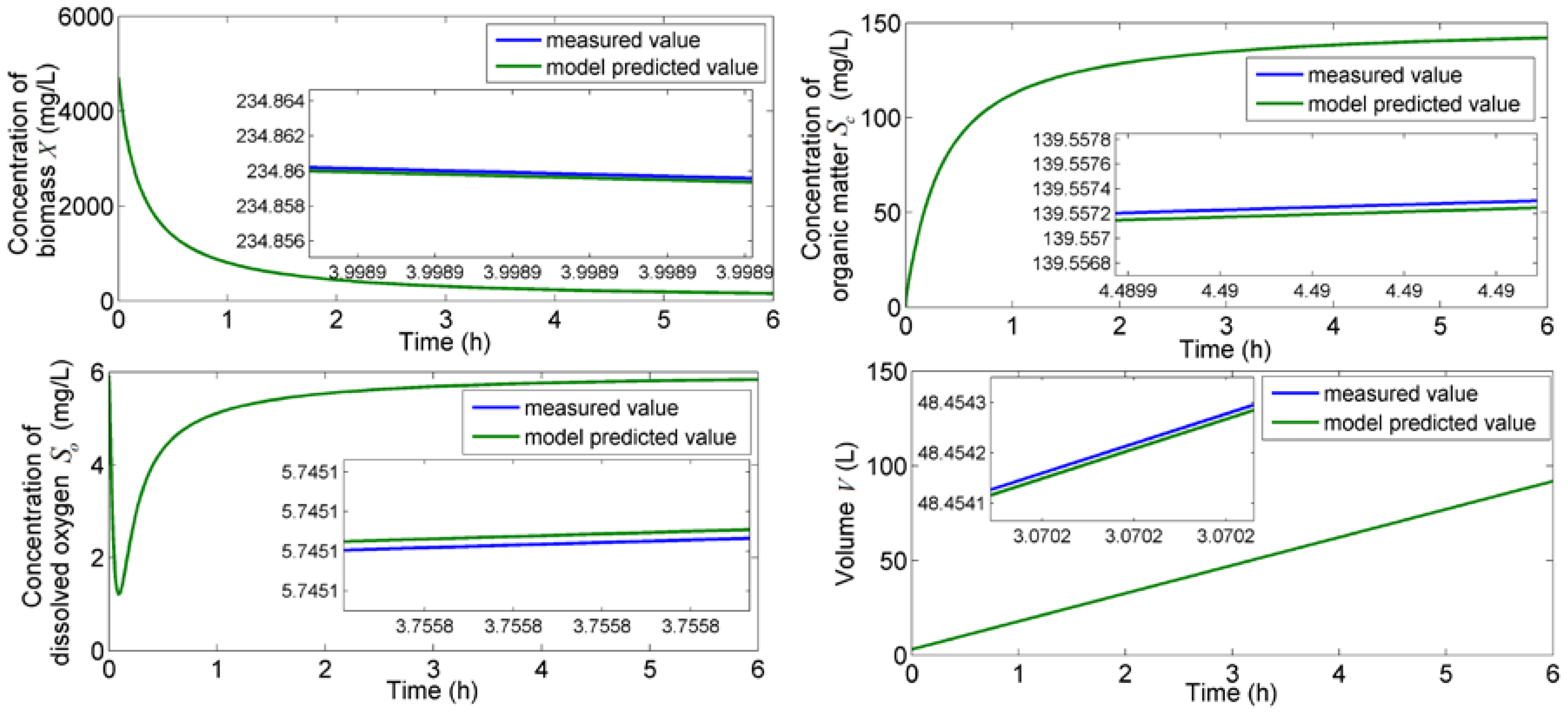
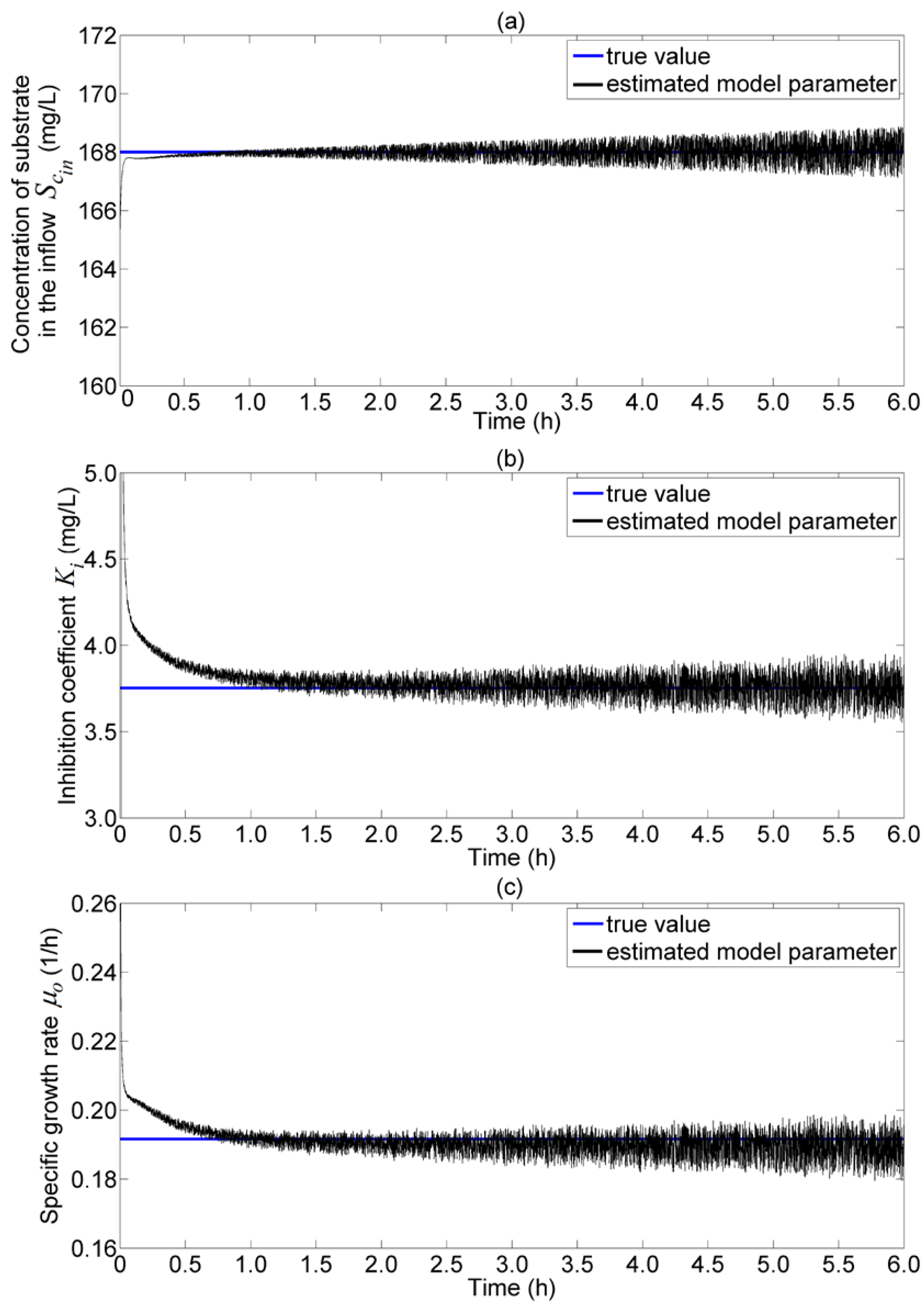
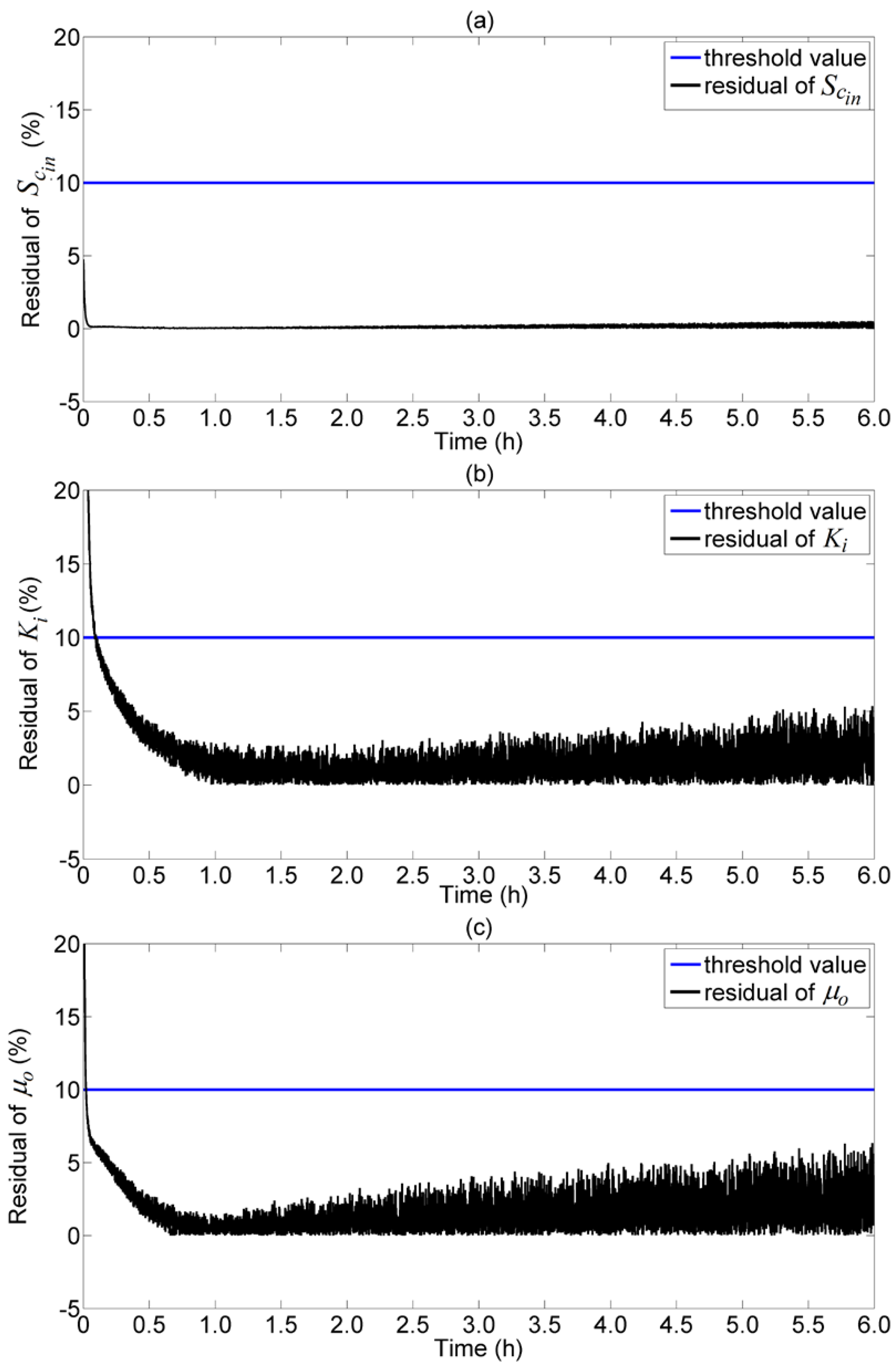
In the fault-free scenario, the simulated measured values and model predicted values for concentrations were obtained using the model parameters listed in Table 1 with initial values, $X(0)=4734$ mg/L, $S_c(0)=0$ mg/L, $S_o(0)=6$ mg/L, and $V(0)=3$ L; the state profiles thus obtained are shown in Figure 2. In this system, noise was added as random data to evaluate the effectiveness of the proposed method. The estimated model parameters, $S_{c_{in}}$, $K_i$, and ${\mu }_o$, were calculated using Equations (39)–(41) with step size, $\Delta t=0.001$ h and are shown in Figure 3. The result shows that the estimated model parameter is close to true model parameters. The diagnosis of fault was carried out by monitoring value of the residual value of model parameters and is shown in Figure 4. For each parameter no fault was detected as the residual was less than the threshold. The threshold was chosen as 10% from the nominal value. These results indicate that the technique proposed in this work can accurately estimate the model parameters, and this was achieved by carrying out simple function evaluations that alleviate the computational burden required for online implementation.

4.2. Faulty Scenario

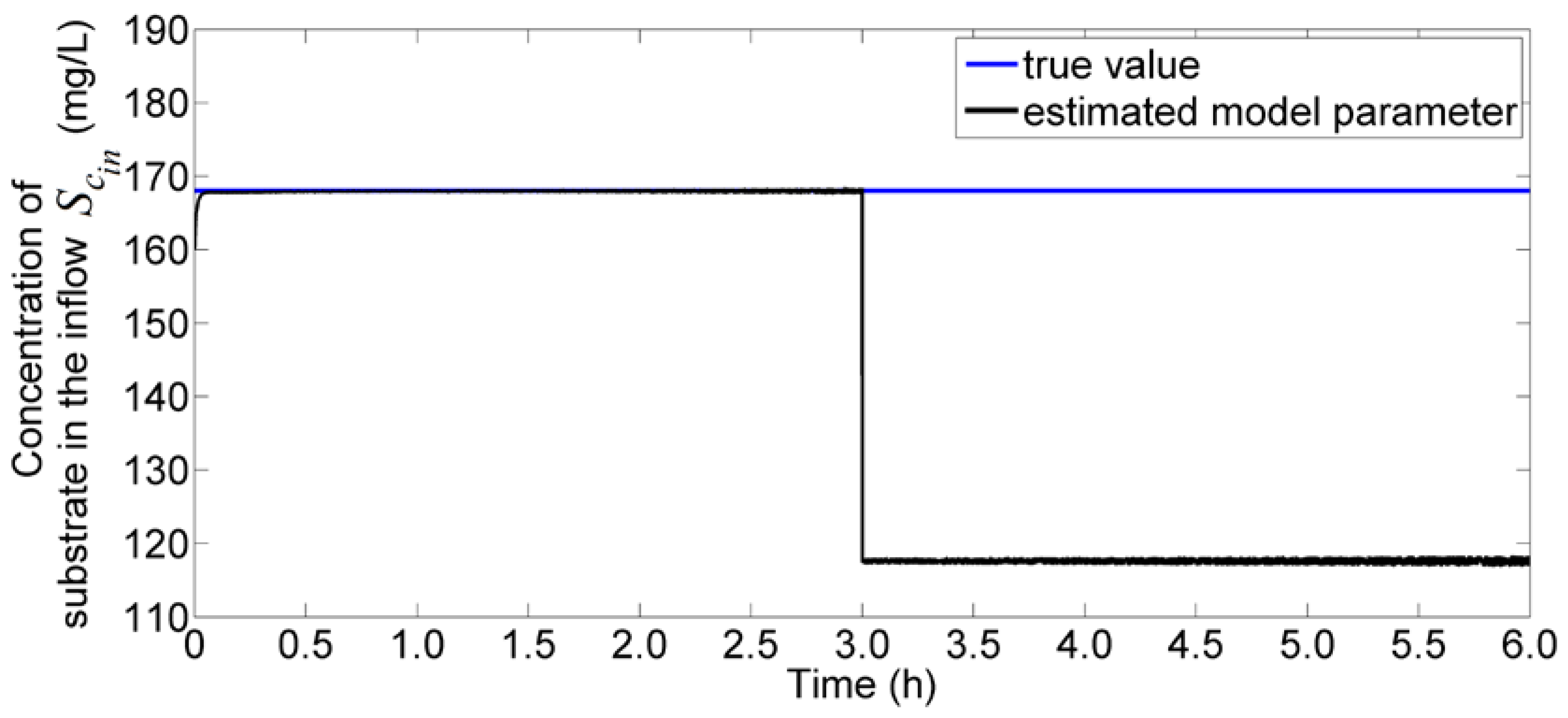
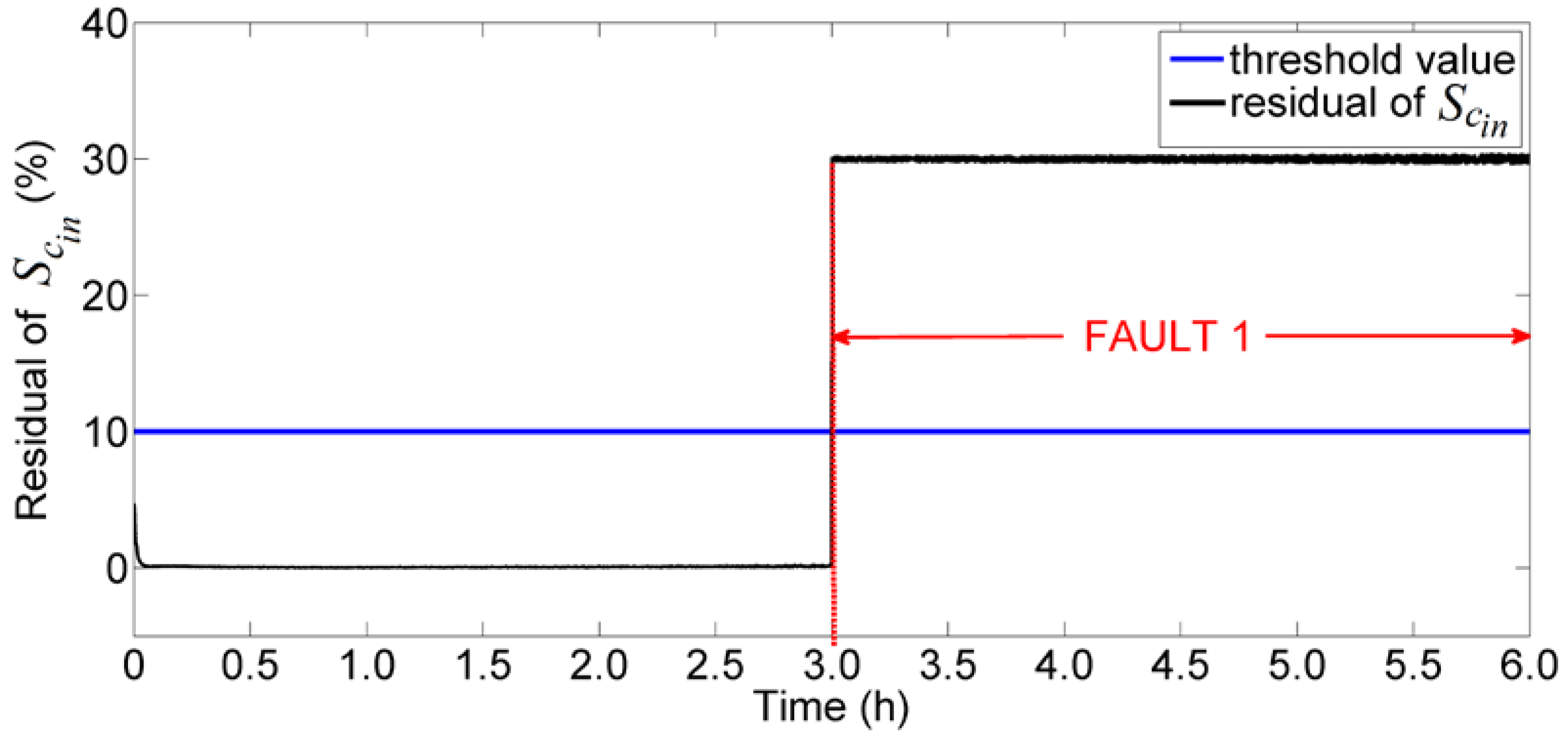
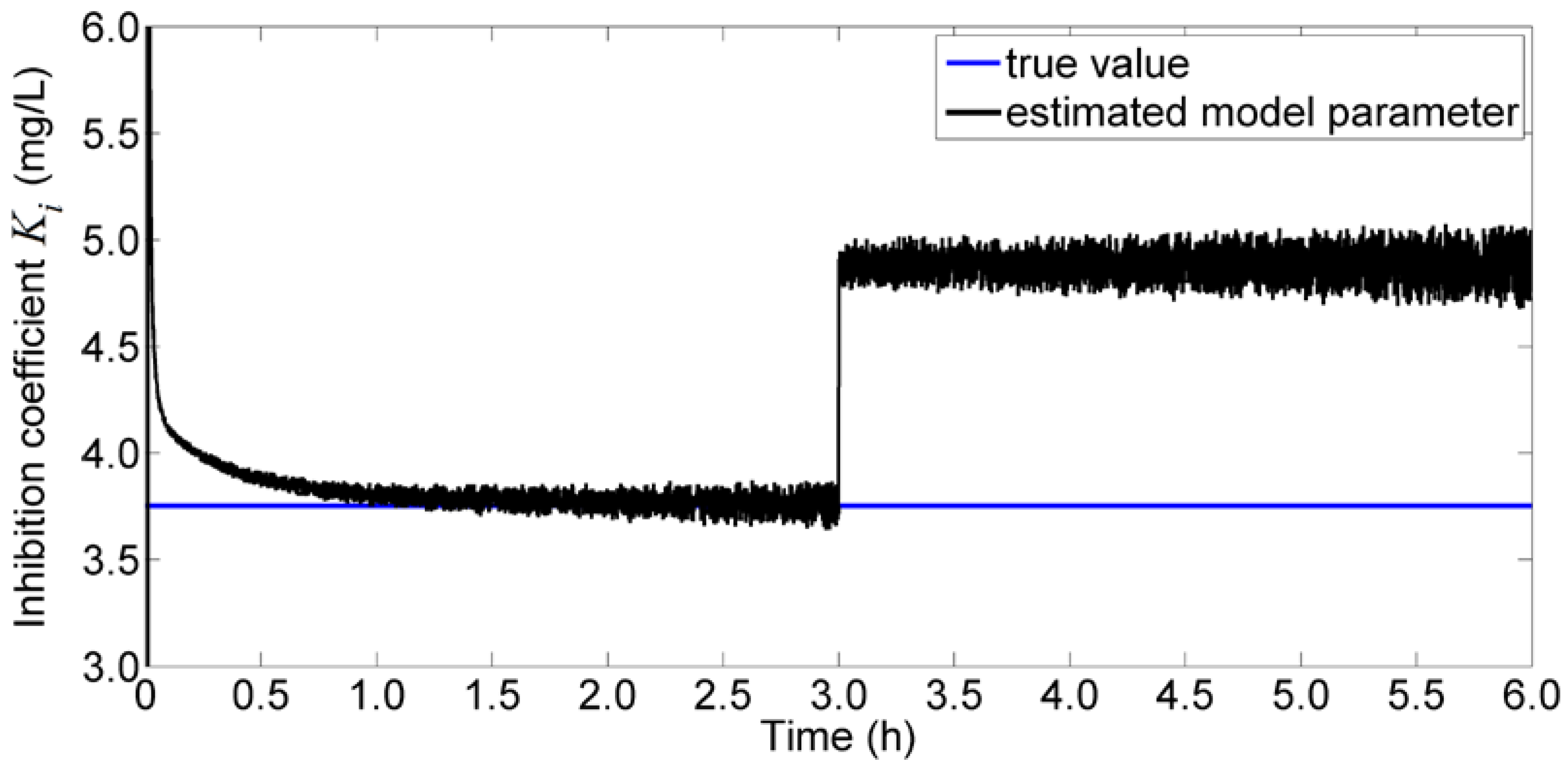
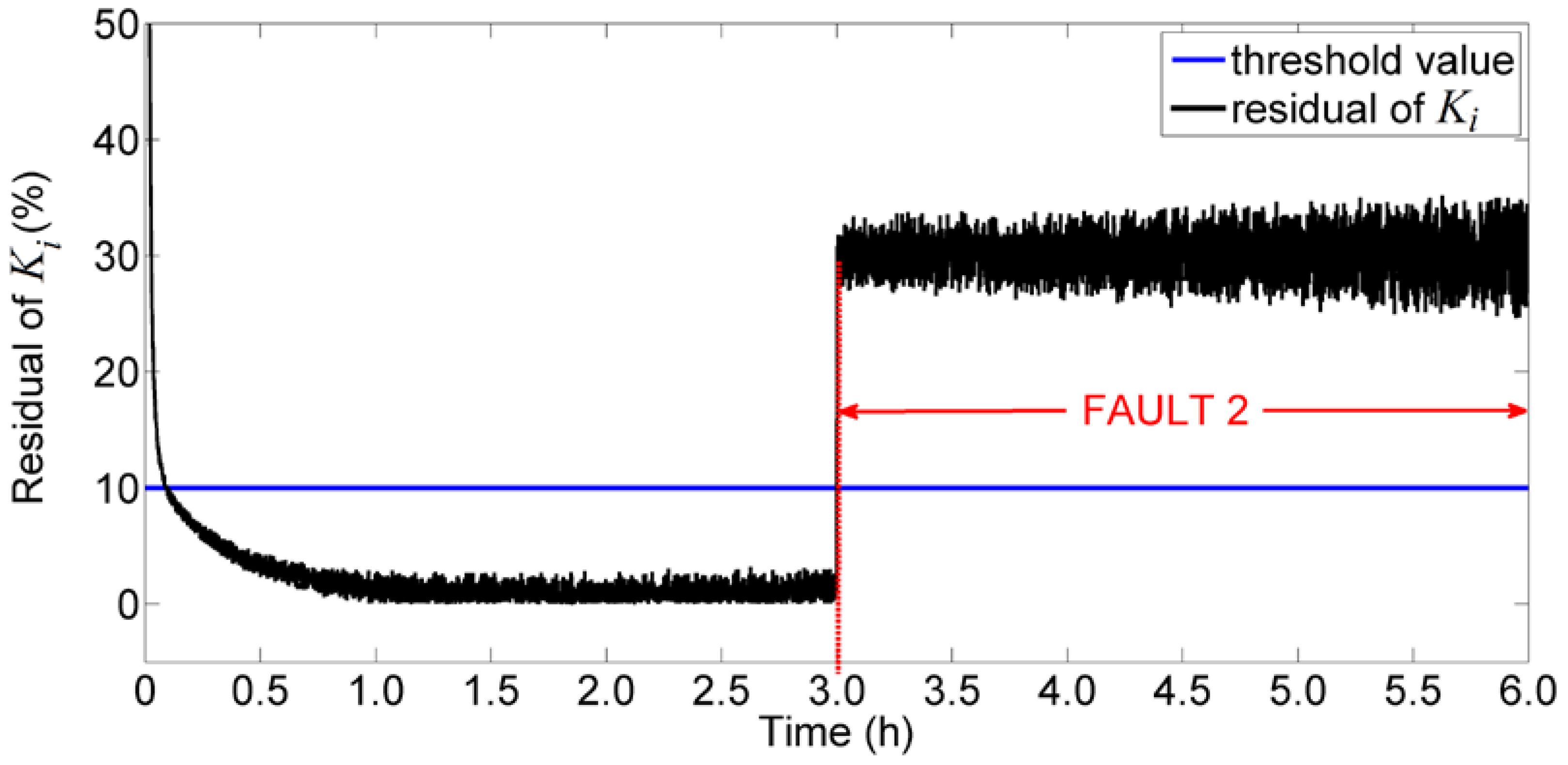
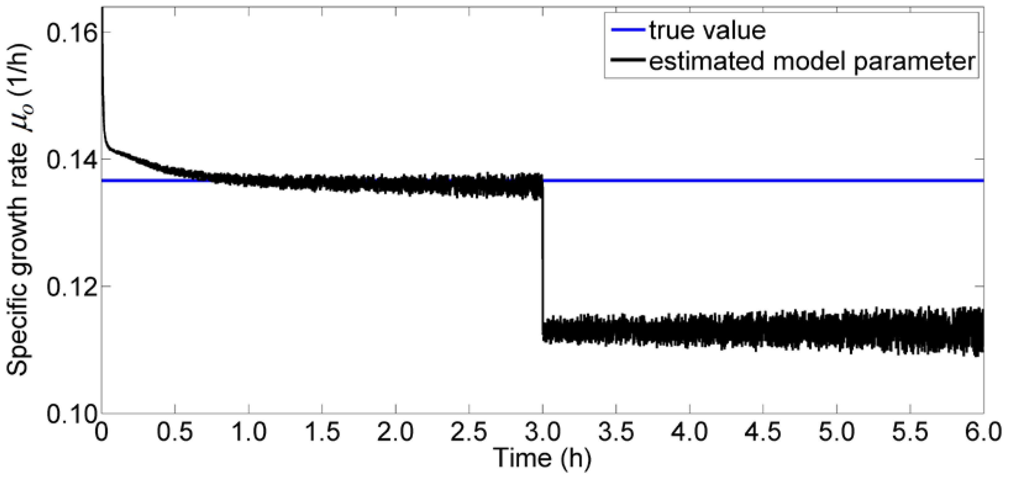
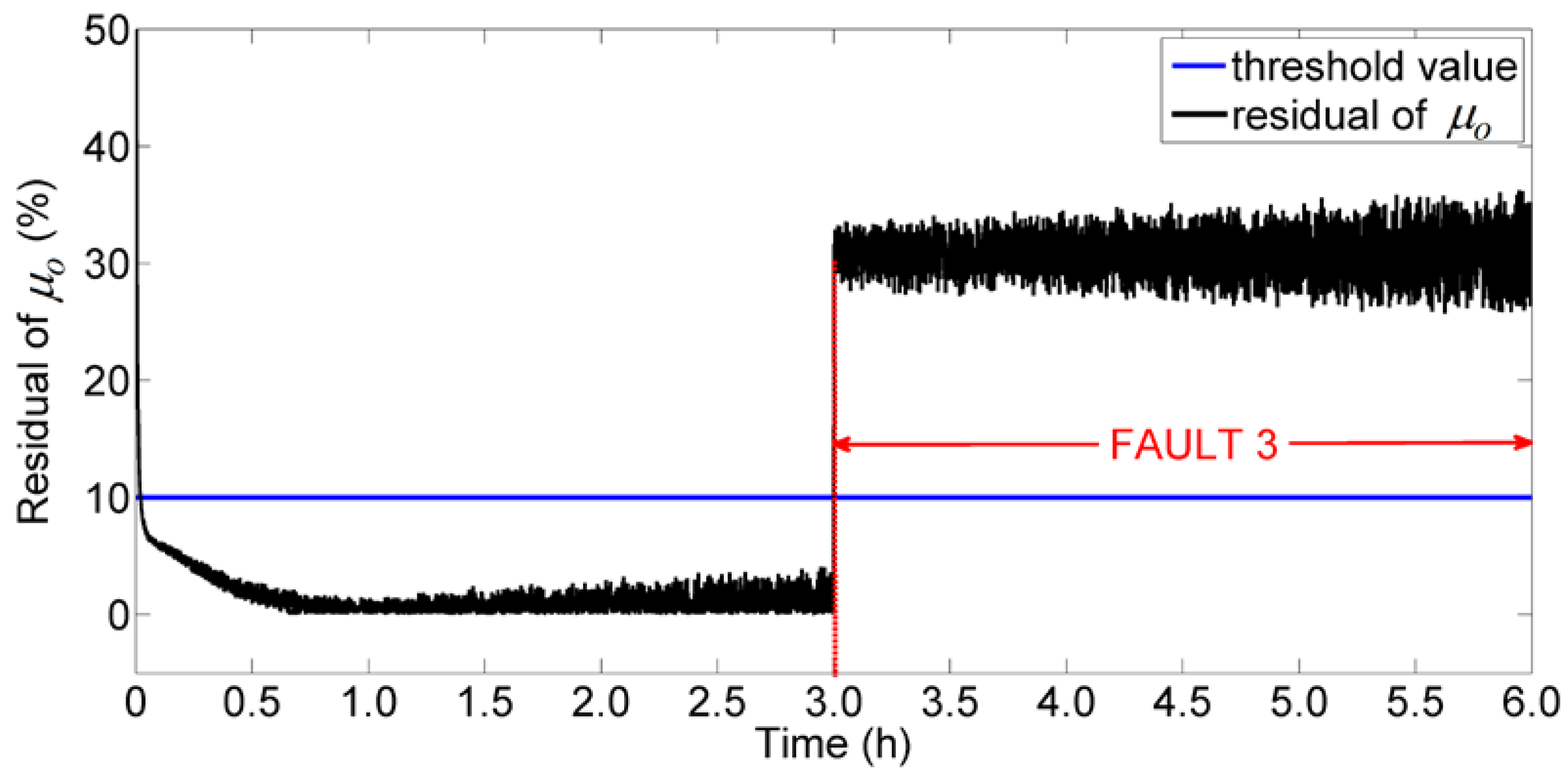
Investigation for the faulty scenarios was implemented where three faulty scenarios have been considered, where the percentage of change kinetic parameters is given in

Table 2. Faulty scenario for the wastewater treatment system.

Fault Kinetic Model Parameter	Fault 1	Fault 2	Fault 3
The concentration of substrate in the inflow, $S_{c_{in}}$	−30%	-	-
The half saturation coefficient, $K_i$	-	+30%	-
Specific growth rate, ${\mu }_o$	-	-	−30%

. In this case study, single fault was assumed to occur at any time. The step size was given as $\Delta t=0.001$ h. For faulty scenario 1, the estimated concentration of substrate in the inflow is shown in Figure 5. We can see that the estimated parameter $S_{c_{in}}$ decreased from 168 mg/L to 118 mg/L after 3 h. The residual of $S_{c_{in}}$ was monitored for fault detection, and is shown in Figure 6. This figure shows that the fault was declared at 3 h as the residual was more than a threshold value of 10%. For faulty scenario 2, the estimated half saturation coefficient, $K_i$, is shown in Figure 7. We can see that the estimated parameter $K_i$ increased from 3.753 mg/L to 4.878 mg/L after 3 h and the residual of $K_i$ was monitored for fault detection. Figure 8 shows that after 3 h, the residual of $K_i$ was more than 10% of threshold and therefore, the fault was declared at 3 h. Figure 9 shows the estimated parameter for ${\mu }_o$ where the estimated model parameter was decreased from 0.1916 1/h to 0.1341 1/h. The fault detection was monitored using residual, and the result is shown in Figure 10. The residual of ${\mu }_o$ increased to 30% and indicates that faulty scenario 3 occurred at 3 h. These results indicate that there were faults at specified scenarios, and provided quick and accurate fault detection using explicit parametric functions.

5. Concluding Remarks

We have proposed a fault detection methodology for the wastewater treatment system using multiparametric programming where the model parameters were efficiently calculated by performing simple function evaluations without solving the online optimization problem. In this work, the related kinetic parameters for the faulty process that were investigated were $S_{c_{in}}$, $K_i$, and ${\mu }_o$, which affected the respiration rate; these kinetic parameters were obtained as an explicit function of measurements. The estimation of kinetic model parameters in faulty and fault-free scenarios has shown good performance in the accuracy of parameter estimation-based fault detection. This demonstrates the advantages of multiparametric programming-based parameter estimation for detecting faults in wastewater treatment plants quickly and accurately, and reducing the online computational burden. Future work will focus on investigating the case when more than one fault simultaneously occurs.

References

- Mo, W.; Zhang, Q. Energy–nutrients–water nexus: Integrated resource recovery in municipal wastewater treatment plants. J. Environ. Manag. 2013, 127, 255–267. [Google Scholar] [CrossRef] [PubMed]
- Tyagi, V.K.; Lo, S.-L. Sludge: A waste or renewable source for energy and resources recovery? Renew. Sustain. Energy Rev. 2013, 25, 708–728. [Google Scholar] [CrossRef]
- Batstone, D.J.; Hülsen, T.; Mehta, C.M.; Keller, J. Platforms for energy and nutrient recovery from domestic wastewater: A review. Chemosphere 2015, 140, 2–11. [Google Scholar] [CrossRef] [PubMed]
- Rosen, C.; Röttorp, J.; Jeppsson, U. Multivariate on-line monitoring: Challenges and solutions for modern wastewater treatment operation. Water Sci. Technol. 2003, 47, 171–179. [Google Scholar] [CrossRef] [PubMed]
- Mhaskar, P.; Gani, A.; El-farra, N.H.; Mcfall, C.; Christofides, P.D.; Davis, J.F. Integrated fault-detection and fault-tolerant control of process systems. AIChE J. 2006, 52, 2129–2148. [Google Scholar] [CrossRef]
- Mhaskar, P.; McFall, C.; Gani, A.; Christofides, P.D.; Davis, J.F. Isolation and handling of actuator faults in nonlinear systems. Automatica 2008, 44, 53–62. [Google Scholar] [CrossRef]
- Du, M.; Mhaskar, P. Isolation and handling of sensor faults in nonlinear systems. Automatica 2014, 50, 1066–1074. [Google Scholar] [CrossRef]
- Maier, H.R.; Dandy, G.C. Neural networks for the prediction and forecasting of water resources variables: A review of modelling issues and applications. Environ. Model. Softw. 2000, 15, 101–124. [Google Scholar] [CrossRef]
- Caccavale, F.; Digiulio, P.; Iamarino, M.; Masi, S.; Pierri, F. A neural network approach for on-line fault detection of nitrogen sensors in alternated active sludge treatment plants. Water Sci. Technol. 2010, 62, 2760–2768. [Google Scholar] [CrossRef] [PubMed]
- Honggui, H.; Ying, L.; Junfei, Q. A fuzzy neural network approach for online fault detection in waste water treatment process. Comput. Electr. Eng. 2014, 40, 2216–2226. [Google Scholar] [CrossRef]
- Lee, J.-M.; Yoo, C.; Choi, S.W.; Vanrolleghem, P.A.; Lee, I.-B. Nonlinear process monitoring using kernel principal component analysis. Chem. Eng. Sci. 2004, 59, 223–234. [Google Scholar] [CrossRef]
- Baggiani, F.; Marsili-Libelli, S. Real-time fault detection and isolation in biological wastewater treatment plants. Water Sci. Technol. 2009, 60, 2949–2961. [Google Scholar] [CrossRef] [PubMed]
- Sanchez-Fernández, A.; Fuente, M.J.; Sainz-Palmero, G.I. Fault detection in wastewater treatment plants using distributed pca methods. In Proceedings of the 2015 IEEE 20th Conference on Emerging Technologies & Factory Automation (ETFA), Luxembourg, Germany, 8–11 September 2015; pp. 1–7. [Google Scholar]
- Garcia-Alvarez, D.; Fuente, M.J.; Vega, P.; Sainz, G. Fault detection and diagnosis using multivariate statistical techniques in a wastewater treatment plant. In Proceedings of the 7th IFAC International Symposium on Advanced Control of Chemical Processes, Istanbul, Turkey, 12–15 July 2009; Volume 42, pp. 952–957. [Google Scholar]
- Chen, A.; Zhou, H.; An, Y.; Sun, W. Pca and pls monitoring approaches for fault detection of wastewater treatment process. In Proceedings of the 2016 IEEE 25th International Symposium on Industrial Electronics (ISIE), Santa Clara, CA, USA, 8–10 June 2016; pp. 1022–1027. [Google Scholar]
- Carlsson, B.; Zambrano, J. Fault detection and isolation of sensors in aeration control systems. Water Sci. Technol. 2016, 73, 648–653. [Google Scholar] [CrossRef] [PubMed]
- Gontarski, C.A.; Rodrigues, P.R.; Mori, M.; Prenem, L.F. Simulation of an industrial wastewater treatment plant using artificial neural networks. Comput. Chem. Eng. 2000, 24, 1719–1723. [Google Scholar] [CrossRef]
- Fragkoulis, D.; Roux, G.; Dahhou, B. Detection, isolation and identification of multiple actuator and sensor faults in nonlinear dynamic systems: Application to a waste water treatment process. Appl. Math. Model. 2011, 35, 522–543. [Google Scholar] [CrossRef]
- Wimberger, D.; Verde, C. Fault diagnosticability for an aerobic batch wastewater treatment process. Control Eng. Pract. 2008, 16, 1344–1353. [Google Scholar] [CrossRef]
- Brouwer, H.; Klapwijk, A.; Keesman, K.J. Modelling and control of activated sludge plants on the basis of respirometry. Water Sci. Technol. 1994, 30, 265–274. [Google Scholar] [CrossRef]
- Carlsson, B.; Lindberg, C.; Hasselblad, S.; Xu, S. On-line estimation of the respiration rate and the oxygen transfer rate at kungsangen wastewater treatment plant in uppsala. Water Sci. Technol. 1994, 30, 255–263. [Google Scholar] [CrossRef]
- Carlsson, B. On-line estimation of the respiration rate in an activated sludge process. Water Sci. Technol. 1993, 28, 427–434. [Google Scholar] [CrossRef]
- Lindberg, C.-F.; Carlsson, B. Estimation of the respiration rate and oxygen transfer function utilizing a slow do sensor. Water Sci. Technol. 1996, 33, 325–333. [Google Scholar] [CrossRef]
- Jiang, T.; Khorasani, K.; Tafazoli, S. Parameter estimation-based fault detection, isolation and recovery for nonlinear satellite models. IEEE Trans. Control Syst. Technol. 2008, 16, 799–808. [Google Scholar] [CrossRef]
- Isermann, R. Fault diagnosis of machines via parameter estimation and knowledge processing—Tutorial paper. Automatica 1993, 29, 815–835. [Google Scholar] [CrossRef]
- Huang, B. Detection of abrupt changes of total least squares models and application in fault detection. IEEE Trans. Control Syst. Technol. 2001, 9, 357–367. [Google Scholar] [CrossRef]
- Garatti, S.; Bittanti, S. A new paradigm for parameter estimation in system modeling. Int. J. Adapt. Control Signal Process. 2012, 27, 667–687. [Google Scholar] [CrossRef]
- Park, S.; Himmelblau, D.M. Fault detection and diagnosis via parameter estimation in lumped dynamic systems. Ind. Eng. Chem. Process Des. Dev. 1983, 482–487. [Google Scholar] [CrossRef]
- Pouliezos, A.; Stavrakakis, G.; Lefas, C. Fault detection using parameter estimation. Qual. Reliab. Eng. Int. 1989, 5, 283–290. [Google Scholar] [CrossRef]
- Venkatasubramanian, V.; Rengaswamy, R.; Yin, K.; Kavuri, S.N. A review of process fault detection and diagnosis part i: Quantitative model-based methods. Comput. Chem. Eng. 2003, 27, 293–311. [Google Scholar] [CrossRef]
- Hwang, I.; Kim, S.; Kim, Y.; Seah, C.E. A survey of fault detection, isolation, and reconfiguration methods. IEEE Trans. Control Syst. Technol. 2010, 18, 636–653. [Google Scholar] [CrossRef]
- Che Mid, E.; Dua, V. Model-based parameter estimation for fault detection using multiparametric programming. Ind. Eng. Chem. Res. 2017, 56, 8000–8015. [Google Scholar] [CrossRef]
- Dua, V.; Pistikopoulos, E.N. Algorithms for the solution of multiparametric mixed-integer nonlinear optimization problems. Ind. Eng. Chem. Res. 1999, 38, 3976–3987. [Google Scholar] [CrossRef]
- Pistikopoulos, E.N.; Dua, V.; Bozinis, N.A.; Bemporad, A.; Morari, M. On-line optimization via off-line parametric optimization tools. Comput. Chem. Eng. 2002, 26, 175–185. [Google Scholar] [CrossRef]
- Pistikopoulos, E.N. Perspectives in multiparametric programming and explicit model predictive control. AIChE J. 2009, 55, 1918–1925. [Google Scholar] [CrossRef]
- Oberdieck, R.; Diangelakis, N.A.; Papathanasiou, M.M.; Nascu, I.; Pistikopoulos, E.N. Pop—parametric optimization toolbox. Ind. Eng. Chem. Res. 2016, 55, 8979–8991. [Google Scholar] [CrossRef]
- Pistikopoulos, E.N.; Georgiadis, M.C.; Dua, V. Multi-Parametric Programming: Volume 1: Theory, Algorithms, and Applications; Wiley-VCH: Weinheim, Germany, 2007. [Google Scholar]
- Pistikopoulos, E.N.; Georgiadis, M.C.; Dua, V. Multi-Parametric Model-Based Control: Volume 2: Theory and Applications; Wiley-VCH: Weinheim, Germany, 2007. [Google Scholar]
- Charitopoulos, V.M.; Dua, V. Explicit model predictive control of hybrid systems and multiparametric mixed integer polynomial programming. AIChE J. 2016, 62, 3441–3460. [Google Scholar] [CrossRef] [Green Version]
- Dua, V.; Dua, P. A simultaneous approach for parameter estimation of a system of ordinary differential equations, using artificial neural network approximation. Ind. Eng. Chem. Res. 2011, 51, 1809–1814. [Google Scholar] [CrossRef]
- Irvine, R.L.; Ketchum, L.H., Jr. Sequencing batch reactors for biological wastewater treatment. Crit. Rev. Environ. Control 1988, 18, 225–294. [Google Scholar] [CrossRef]
- Fibrianto, H.; Mazouni, D.; Ignatova, M.; Herveau, M.; Harmand, J.; Dochain, D. Dynamical modelling, identification and software sensors for sbrs. Math. Comput. Model. Dyn. Syst. 2008, 14, 17–26. [Google Scholar] [CrossRef] [Green Version]
Figure 1.
The sequencing batch reactor stages (adapted from Reference [41]).
Figure 2.
State variables profiles for the fault-free scenario.
Figure 3.
Estimated model parameters value for the fault-free scenario. (a) Concentration of substrate in the inflow, ; (b) inhibition coefficient, ; and (c) specific growth rate, .
Figure 4.
Residual of estimated model parameters for the fault-free scenario. (a) Concentration of substrate in the inflow, ; (b) inhibition coefficient, ; and (c) specific growth rate, .
Figure 5.
Estimated model parameter for faulty scenario 1.
Figure 6.
Residual of the estimated model parameter for faulty scenario 1.
Figure 7.
Estimated model parameter for faulty scenario 2.
Figure 8.
Residual of the estimated model parameter for faulty scenario 2.
Figure 9.
Estimated model parameter for faulty scenario 3.
Figure 10.
Residual of the estimated model parameter for faulty scenario 3.