Surrogate Models for Online Monitoring and Process Troubleshooting of NBR Emulsion Copolymerization

Abstract

Chemical processes with complex reaction mechanisms generally lead to dynamic models which, while beneficial for predicting and capturing the detailed process behavior, are not readily amenable for direct use in online applications related to process operation, optimisation, control, and troubleshooting. Surrogate models can help overcome this problem. In this research article, the first part focuses on obtaining surrogate models for emulsion copolymerization of nitrile butadiene rubber (NBR), which is usually produced in a train of continuous stirred tank reactors. The predictions and/or profiles for several performance characteristics such as conversion, number of polymer particles, copolymer composition, and weight-average molecular weight, obtained using surrogate models are compared with those obtained using the detailed mechanistic model. In the second part of this article, optimal flow profiles based on dynamic optimisation using the surrogate models are obtained for the production of NBR emulsions with the objective of minimising the off-specification product generated during grade transitions.

1. Introduction

Nitrile butadiene rubber (NBR) is an elastomer used in a wide variety of applications demanding oil, fuel and chemical resistance where the content of acrylonitrile influences the end use. NBR can be produced by emulsion copolymerization of acrylonitrile (AN) and butadiene (Bd) using batch, semi-batch, and continuous processes. Usually it is produced using a series of eight to ten continuous-stirred tank reactors (CSTRs). Cold NBR polymers are synthesized between 5 and 15 °C, while hot NBR polymers are usually synthesized between 30 and 50 °C. A comprehensive mechanistic model that can predict different property trajectories for NBR emulsion polymerization has been developed by our group and has been successfully verified with experimental results over a long period [1,2,3]. This model is capable of simulating the emulsion polymerisation of NBR in batch and in a train of CSTRs, with add-on options, such as choosing the type of reactor start-up, different modes of monomer partitioning, and the effect of impurities. More detailed information regarding the traits and attributes of this model can be obtained elsewhere [4,5]. The mechanistic model developed by our group is complete and comprehensive and has been used for more than just obtaining the simulated dynamic behavior of commercial trains of CSTRs corresponding to different operating conditions. Depending on the type of start-up of the reactor train and different mechanisms selected by the user to be operative (related to radical desorption, partitioning methods, etc.), the simulation time varied from several minutes to an hour. In the case of starting up the reactors full of water or empty, the simulation time was found to be almost two hours, depending on the detail of the selected thermodynamic approach for monomer partitioning. To integrate the process model for control and optimisation applications, though, the current mechanistic model can be used, as it adds significant delay in the response of the measured variables before the control action is taken. To overcome this problem, suitable surrogate models (whose order is significantly less than the order of the actual mechanistic model and whose simulation times are far less than that of the fully mechanistic model) are proposed and used in this article for further online applications. The objective of the current article is two-fold: firstly, we explain the need for using surrogate models (in addition to the detailed model developed by our group), obtained using various techniques such as neural networks and transfer function models; secondly, we use them for real-time process applications, such as recipe formulations, control, and dynamic optimisation.

Surrogate models can come to the rescue when the objective is to control or optimise a process whose dynamics are either complex or involves relatively tedious and time-consuming numerical analysis to solve the original complex model for obtaining different state variables, or when the actual physics/chemistry of the process are poorly understood/not known. Artificial neural networks (ANN) are an important and useful tool that belongs to the class of surrogate modeling and is used for control and optimisation of processes which are highly nonlinear [6,7]. Several authors have reported using ANN alone for predicting dynamic behavior or for controlling polymerization reactors [8,9], or otherwise, in a hybrid mode where ANN is used in addition to the corresponding simpler mechanistic model of the system [10,11]. In general, ANNs are highly efficient when trained with large datasets involving a wide range of operating conditions. Otherwise, their performance will be limited and their predictions will be different from the expected dynamics [11]. With sufficient training data, ANN can efficiently be used for prediction of steady state properties as reported by Vijayabhaskar et al. [12], Assenhaimer et al. [13], and Delfa and Boschetti [14]. For emulsion copolymerisation systems. Although ANNs are used like a black box for modeling processes that are nonlinear, very little is available in the literature for using them as inverse modeling tools for complex polymerisation processes. In the current article, an inverse modeling approach with ANNs based on the back propagation technique is used for obtaining formulations for recipe ingredients to be used in the first reactor of the train that will give desired properties of the copolymer in the last reactor of the train (in a continuous mode). To further illustrate the points and shed more light, the capability of ANNs to predict the dynamic behaviour of emulsion copolymerisation of NBR in a batch reactor is described and discussed next. A major contribution of this research article (in addition to using ANNs) is to discuss how transfer function models are obtained for emulsion copolymerisation of NBR. For the first time, a complex process like the NBR system is described using transfer functions, which are, in turn, used for controlling the properties of the final product.

2. ANNs for NBR Emulsion Copolymerization in a Batch Reactor

In this section we explain how ANNs are used to simulate the production of NBR emulsion copolymerisation in a batch reactor. With the mechanistic model, the overall simulation time strongly depended on several factors such as the type of method for calculating monomer partitioning (i.e., thermodynamics vs constant partition coefficients), presence of monomer or water soluble impurities, and other details in the copolymerization kinetics. For any fast control action to be taken, relying on the mechanistic model would be equivalent to adding a dead time or delay to the measurement signal, the typical fast measurement being on conversion (X), with other rather slow measurements on copolymer composition or particle size or Mooney viscosity. Mooney viscosity is a well-known indirect measure of an average molecular weight of a polymer (usually a rubber product), determined by a Mooney visometer. In batch operation, ANN is designed to predict the effect of time on important latex and polymer properties such as conversion, number of particles, copolymer composition (CPC), weight-based and number-based average molecular weights, and tri- and tetra-functional branching frequencies. In the simulations, ANN based on back-propagation is programmed in MATLAB, where the total prediction error, $E(\underset{¯}{W})$ (given by Equation (1)), is minimized. The error, $E(\underset{¯}{W})$, also referred to as quadratic error, is defined as the sum of the squares of the differences between the desired output, Y_i, and the predicted output, X_i. The predicted output X_i, is a function of the weights (W_jk for one hidden layer) used in the network, where the subscripts j and k represent the indices of the input and output neurons. In vector notation, W_jk is usually represented by $\underset{¯}{W}=(W_{12},W_{13},W_{14},\mathrm{...})$:

$$E(\underset{¯}{W})=\frac{1}{2}{\displaystyle \sum {[Y_i-X_i(\underset{¯}{W})]}^2}$$

(1)

The predicted output is operated upon by an activation function also known as a squashing function. The two most commonly used activation functions are the sigmoid and hyperbolic tangent. It should be noted that, in the absence of the activation function, the problem reduces to that of a multiple linear regression model. It is the activation function that provides the ability to handle nonlinearities. The best values for the weights, W_jk, are obtained by training the network using Levenberg–Marquardt back-propagation algorithm. In this algorithm, the weights are adjusted using the method of steepest descent with respect to the error E, as defined by Equation (1). The builtin function, trainlm.m, in MATLAB is based on this algorithm and is used in the simulations for the NBR system. The desired output, Y, is obtained from the mechanistic model, which gives good predictions when compared with the experimental data, as established in previous work [4,5]. The original mechanistic model is highly nonlinear with 32 multiscale state variables. The data obtained from the mechanistic model are divided into training, validation, and untested datasets (also called unseen datasets). From the available data sets, 70% of the data is used for training, 15% percent of the data is used for validation, and the remaining 15% of the data is used for testing. To avoid an overfitted model for the training data, a program in MATLAB is written for obtaining the optimum size and complexity of the network with the objective that the training error be comparable to the prediction error. Performance characteristics of the designed ANN for the prediction of conversion, cumulative copolymer composition (CPC), weight-based average molecular weight (MW_w) and tri-functional branching frequency (BN₃) are shown in Figure 1a–d. In these figures, the profiles obtained from the mechanistic model (MM) are compared to those obtained using ANN for a targeted batch time of 700 min (a typical value used in commercial production). A very good agreement was achieved between the predictions using ANN with those obtained using the well-established and tested MM. The designed ANN for NBR emulsion copolymerisation in a batch reactor can, thus, be safely used in conjunction with process control and optimisation algorithms for describing the desired properties of the polymer.

3. ANN for Inverse Modeling of NBR Emulsion Copolymerisation in a Train of CSTRs

NBR is commercially produced in a continuous fashion using eight to ten reactors operated in series. Depending on the demand, a CSTR can be added or removed from the series, which indirectly affects the mean residence time of the train of CSTRs. The properties of the product from the last reactor are affected by the recipe ingredients used in the first reactor of the train and by the operating conditions of the train. While ANNs can be used to predict these properties based on recipe ingredients given as inputs, by using ANN-based inverse modeling, the recipe ingredients to be used in the first reactor for targeted properties exiting the last reactor can be obtained. This is achieved by using the properties of the product from the last reactor (say, the eighth reactor in an eight-reactor CSTR train) to be the inputs to the network, while the outputs are the recipe ingredients to the first reactor. This type of inverse modeling is easy and efficient with ANNs compared to the alternative, i.e., offline optimisation using the corresponding mechanistic model as a constraint. The ingredients that are fed to the first reactor are initiator (I), reducing agent (RA), emulsifier(s) (E), monomer(s) (M), water (W), and chain transfer agent (CTA). Considering typical high and low levels for each one of these reaction ingredients, the corresponding conversion (X), cumulative copolymer composition (CPC), and the weight-based average molecular weight (MW_w) at the exit of the eighth reactor can be simulated using the mechanistic model. Out of the 64 available datasets, 52 datasets are then used for training the network and 12 datasets are left in order to check the performance of the ANN with respect to inverse modeling of the recipe ingredients for obtaining the desired polymer properties. The different levels of the reaction ingredients used for MM simulations are shown in

Table 1. Recipe ingredients to the first reactor in the reactor train and their levels.

Ingredient	Low Level (L/min)	High Level (L/min)
Sodium Formaldehyde Sulfoxylate (RA)	0.165	0.22
p-methane hydroperoxide (I)	0.046	0.062
Dresinate/Tamol (E)	0.89/1.67	1.183/2.228
Acrylonitrile/Butadiene (M)	48.6/160.3	64.8/213.7
Water (W)	121.36	161.81
tert-dodecyl Mercaptan (CTA)	0.33	0.44

Note: Mean residence time of each reactor in train is 60 min.

. The low and high levels of the reaction ingredients can be normalized to −1 and +1, respectively which, in turn, are used as outputs from the network. The inputs to the network, as shown in Figure 2, are X, CPC, and MW_w, while the outputs are the recipe ingredients RA, I, E, M, W, and CTA.

With the objective of obtaining the minimum mean sum of squared errors (MSE), simulations were performed to study the effect of the number of hidden layers and the number of neurons in each layer.

Table 2. Effect of number of hidden layers and number of neurons on MSE.

Number of Neurons	Number of Hidden Layers
	Monomer			CTA
	1	2	3	1	2	3
5	0.1532	0.1593	0.0033	0.1370	0.0420	0.0405
10	0.0653	0.0289	0.0836	0.0677	0.0509	0.2600
15	0.0148	0.0659	0.0405	0.0143	0.2070	0.1355
20	0.0245	0.2412	0.0124	0.137	0.1175	0.0613

shows the MSE values for monomer and CTA concentrations obtained by varying the number of hidden layers from one to three and the corresponding number of neurons in each layer from five to 20. All ANN simulations took less than 3 s for obtaining the trained networks. As is evident from Table 2, a network with three hidden layers and 20 neurons gives minimum MSE values and the same trend was found for other reaction ingredients (I, RA, W, and E).

A possible reason that can be attributed to the resulting large network is that the difference in the magnitude for the output variables such as conversion and weight-based molecular weight is almost 10⁶. Hence, the optimum configuration used in this work was a network with three hidden layers with 20 neurons in each layer. Though the number of weights for such a large network is very high, the simulation time for obtaining the trained network in all simulations was only a few seconds. The trained network (saved as .MAT file in MATLAB) in turn is used as an inverse modeling tool to predict the recipe ingredients (of the first reactor) for targeted properties of the stream exiting the eighth reactor. Figure 3 (a through f) shows the recipe ingredients’ predictions obtained using the ANN-based inverse modeling for desired conversion (X) compared to the data obtained from the mechanistic model. The proposed ANN-based inverse modeling could predict the required recipe ingredients very well for desired conversion levels. Similar results and trends were obtained for desired CPC and MW_w (as shown in Figure 4 and Figure 5). The predictions for all reaction ingredients are precise, except for the initiator in some cases. The prediction capability of the ANN can be quantified using the mean sum of squared errors (MSE) for each dataset. The MSE values for each of the predicted datasets are shown in

Table 3. MSE values for the 12 untested datasets using ANN.

#	X	CPC	MWw		Mean Squared Error (MSE)
				RA	I	E	M	W	CTA
1	0.5611	0.2573	1.17 × 105	0.1247	2.7766	0.0136	0.0105	0.1115	0.0255
2	0.7668	0.2811	1.51 × 105	0.0096	4.0446	0.0074	0.0042	0.0240	0.0001
3	0.4743	0.2735	8.54 × 104	0.0518	5.6491	0.0384	0.0014	0.0016	0.0068
4	0.5515	0.2285	7.56 × 104	0.2717	0.2051	0.7459	0.0300	0.0110	0.1170
5	0.7669	0.2811	1.95 × 105	4.1140	1.4764	0.0101	0.0015	0.0002	0.0396
6	0.6454	0.2711	1.19 × 105	5.2109	4.4500	2.6381	0.0287	0.0034	0.1231
7	0.5689	0.2349	1.05 × 105	0.1591	8.3361	0.0016	0.0076	0.3575	0.1394
8	0.4246	0.2676	5.45 × 104	0.0674	2.9982	0.0549	0.0037	0.0053	0.0211
9	0.6895	0.2784	1.80 × 105	0.0325	2.6604	0.0100	0.0094	0.0000	0.0626
10	0.7074	0.2713	1.24 × 105	0.0470	4.2123	0.0217	0.0001	0.0024	0.0424
11	0.4247	0.2676	7.22 × 104	0.0743	2.9586	0.0487	0.0206	0.0027	0.1336
12	0.6703	0.2547	1.16 × 105	0.0014	2.6040	0.0243	0.0321	0.0004	0.0246

.

The MSE values from Table 3 clearly show that the prediction using ANN-based inverse modeling is precise for almost all reaction ingredients except for the initiator. The obtained the MSE of the initiator is slightly greater than the MSE values of the other reaction ingredients. This is due to the fact that the magnitude of initiator concentration is very small compared to the concentrations of the other ingredients. The above results show that ANN-based inverse modeling can give good estimates of the reaction ingredients to be used in the first reactor (which can be applied to batch reactor operation as well) for obtaining the desired properties of the polymer exiting the last reactor of the CSTR train. This method of obtaining the estimates (for initial reaction ingredients) is easier and less time consuming compared to using the fully mechanistic model. Using the mechanistic model (which is very useful in its own right, as we have shown in previous publications, e.g., Madhuranthakam and Penlidis [4,5]), a trial and error approach has to be used for initial reaction ingredients. During the operation of the reactor train, for any slight discrepancies in the desired properties of the products, it is always possible to fine-tune the estimates obtained using the ANN-based inverse modeling.

4. Surrogate Modeling for NBR Emulsion Copolymerization

In this section, models that are capable of predicting the dynamics and are amenable for control and/or optimisation applications for the emulsion copolymerisation of NBR are discussed. The ANNs discussed in the previous sections can also be used for predicting the dynamics and for control purposes, but the additional benefit of the surrogate models is that these models in their standard forms, such as a first order plus time delay or a second order plus time delay, etc., have fewer parameters than the number of weights obtained using the ANN. In many situations, the parameters of a feedback controller or a model predictive controller can be obtained as functions of the corresponding parameters of the model, which is not feasible with the case of ANN. Surrogate models are obtained by reducing the order of the original mechanistic model so that computation of the dynamic behaviour is fast, which in turn helps with online control and optimisation applications. Depending on the type and order of the original model, the model can be reduced either by using a model balancing approach or by error minimization. Model balancing involves evaluating the controllability and observability Gramians and partitioning the state vector into important states and less important states. The reduced model is obtained by truncation of the least important states [15]. This method involves linearizing the original model around an operating condition or empirically obtaining Gramians corresponding to each operating condition, which may be very tedious. The actual mechanistic model for NBR emulsion copolymerization includes 32 state variables and its highly nonlinear nature makes it cumbersome to obtain a corresponding linearized model. Due to this reason, empirical models are obtained by using error minimization criteria. The initial choice of type of empirical models is very crucial as there could be multiple models (which could differ in the number of parameters) that can fit equally well the corresponding data available. After choosing a specific transfer function model, the models are fine-tuned later based on the objective of minimizing the error between the responses of the proposed empirical model and the data (obtained from the mechanistic model). The parameters of the final surrogate model are obtained by simulation and using the nonlinear least squares fitting function lsqnonlin in MATLAB.

5. Transfer Function Models for the First CSTR in the Reactor Train

As mentioned in the previous sections, the ingredients entering the first CSTR are the initiator, emulsifier(s), monomers, water, and chain transfer agent streams. Typical outputs considered for obtaining the corresponding surrogate models are conversion, cumulative copolymer composition, weight-based average molecular weight, and the total number of latex particles per liter of water (N_p). These are the typical outputs (in principle, measurable) which are, in turn, used in the controlled production of NBR latex. Surrogate modeling is conducted in the Laplace domain by programming interactive simulations between SIMULINK and MATLAB. The performance of the corresponding fitted transfer function model is evaluated in terms of the coefficient of determination, R². The input variables chosen to be related to any output variable are restricted to the states that have higher impact than others and that can also be used as practical manipulated variables in control applications. For example, when the reactor is started full of batch recipe (for other types of start-up policies refer to [4]), the conversion obtained at the exit of the reactor is expressed as a function of initiator, and acrylonitrile and butadiene (monomers) flow rates, as shown in Equation (2):

$$Y_1(s)=\frac{\frac{{\tau }_2}{K_1}s}{{\left(\sqrt{\frac{{\tau }_1{\tau }_2}{K_1}}\right)}^2{s}^2+((1+K_1){\tau }_2)s+1}{X}_1(s)+\frac{K_1}{{\tau }_{2}s+1}{X}_2(s)+\frac{K_1}{{\tau }_{2}s+1}{X}_3(s)$$

(2)

where Y₁ denotes conversion, X₁ represents initiator flowrate, X₂ is the acrylonitrile flow rate, and X₃ is the butadiene flow rate, all in the Laplace domain. τ₁, τ₂, and K₁ are the parameters of the model. Since the input and output variables in the transfer function models represent perturbations from initial steady states, the final model constitutes an initial value problem with all variables (outputs) to be zero at time t = 0. The structure of this model basically consists of a combination of a second order and two first order systems. The parameters τ₁, τ₂, and K are obtained by fitting the model response to the data obtained from the mechanistic model for a given step change in the input variables X₁, X₂, and X₃. Similarly, for other output variables such as CPC (Y₂), MW_w (Y₃), and N_p (Y₄), the corresponding models are given by Equations (3)–(5):

$$Y_2(s)=\frac{K_2}{{\tau }_{3}s+1}\exp (-{\tau }_{4}s)X_4(s)$$

(3)

$$Y_3(s)=\frac{K_{3}s+1}{{\tau }_5^2{s}^2+2{\tau }_5{\tau }_{6}s+1}{X}_5(s)$$

(4)

$$Y_4(s)=\frac{K_{4}s}{{\tau }_7^2{s}^2+2{\tau }_7{\tau }_{8}s+1}{X}_1(s)+{\left[\frac{1}{{\tau }_{7}s+1}\right]}^2{X}_6(s)$$

(5)

where Y₂, Y₃ and Y₄ represent the output variables CPC, MW_w, and N_p, respectively, whereas X₄, X₅, and X₆ represent the ratio of flow rates of the two monomers (AN to Bd), chain transfer agent flow rate, and emulsifier flow rate, respectively. K₂, K₃, K₄, and τ₃ through τ₈ are parameters of the empirical models. Equations (2)–(5) represent the empirical surrogate models for the dynamics of the first reactor in the reactor train. When the reactor is started full of recipe, the inflow to the first reactor is equivalent to giving a step input to all input variables X₁ through X₆ and the output responses Y₁ through Y₄ are used to obtain the corresponding parameters of the empirical models. The final comparison of the responses obtained for X, CPC, MW_w, and N_p using the data from the mechanistic model (MM) and the proposed empirical models (EM) are shown in Figure 6a–d, respectively.

The proposed empirical models fit very well the data obtained from the mechanistic model is evident from the very high R² values (close to unity) reported on the corresponding figures. Since the weight-based average molecular weight (MW_w) in the mechanistic model is obtained from a set of very highly nonlinear model equations that originate using the method of moments, the corresponding empirical model had a lower R² value compared to the values of the other output variables. In general, the performance of the surrogate models is very good. The proposed empirical models are not only simple and amenable to use for online purposes but also have very few parameters. With the success of using this method for a single CSTR (the first reactor of the CSTR train), the properties at the exit of the eighth reactor can also be empirically modeled and further used in online applications, such as control and grade transitions.

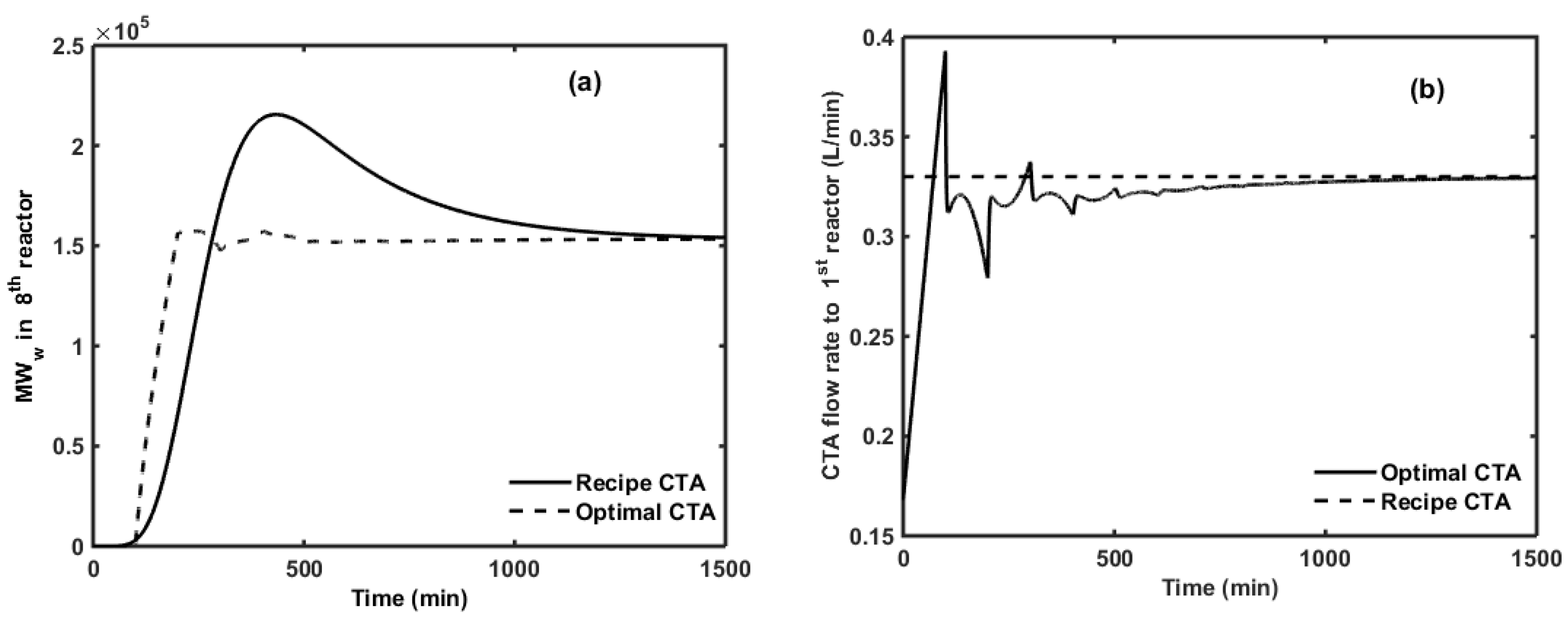
6. Optimal CTA Profile for Minimizing off-Spec Product

The weight-based molecular weight response exiting the eighth reactor in the reactor train is empirically modeled using the knowledge of the corresponding dynamics in the first reactor of the train. The validity and versatility of the proposed empirical model is shown in Figure 7 where two different reactor start-up procedures are used (one of them starting the reactor train full of recipe (Figure 7a) and the other starting full of water (Figure 7b). The empirical model obtained for this case is given by Equation (6).

$$Y_8(s)={\left[\frac{Ks+1}{{\tau }_1^2{s}^2+2{\tau }_1{\tau }_{2}s+1}\right]}^8{X}_5(s)$$

(6)

Y₈ is the MW_w obtained at the exit of the eighth reactor, X₅ is the flow rate of the CTA to the first reactor in the reactor train, and K, τ₁, and τ₂ are model parameters. The empirical model consists of eight second-order transfer functions in series, each of them corresponding to the dynamics of each individual reactor in the reactor train. From the R² values reported in Figure 7a,b, it is evident that the proposed second order transfer function in series fits very well the corresponding mechanistic model in addition to the benefit of employing three parameters only (K, τ₁, and τ₂).

One of the most common operational constraints that occur in the commercial production of NBR is during grade changes. During grade changes, the reactor train is switched to operate from one steady state to another desired steady state. These can be viewed as set point changes that occur due to customer or production campaign requirements. One of the primary objectives during grade changes or for start-up of the reactor train is to minimize the off-specification product that is produced before reaching the steady state. The off-specification product can be minimized in multiple ways but a usual practice is to add intermittent flows of the manipulated variables along the reactor train in a feedforward fashion where the magnitudes of the flow rates of the manipulated variables are estimated by performing offline optimisation. For batch and semi-batch production of polymers, Fujisawa and Penlidis [16] have shown different reactor control policies targeted for obtaining desired copolymer compositions using an offline mechanistic model. For reducing transients during grade changes for NBR and styrene butadiene systems, Minari et al. [17,18] have used a bang-bang method (which also uses an offline mechanistic model), where predetermined quantities of CTA and monomer are added along the reactor train in one shot to reduce the molecular weights and the CPC in the last reactor of the reactor train. In the present work we propose an online method, where continuous profiles for manipulated variables such as CTA, monomers etc. are obtained using dynamic optimisation. This method assumes that the information for molecular weight becomes available online via an inferential estimator based on Mooney viscosity, in order to minimize the time delay related to the measurement of molecular weight. The empirical model (as given be Equation (6)) can be used either online or offline optimisation when there is a grade change with respect to MW_w. For simultaneous control of conversion, CPC, and MW_w, a multiobjective function based on a weighted sum or ε-constrained methods can be used [19,20]. While grade changes can involve an increase or decrease in several product specifications, such as conversion, CPC, N_P, MW_w, etc., the application to the scenario where a decrease in MW_w by adding extra CTA to the reactor train is discussed here as an example. In general, the inflows to the last few reactors are manipulated rather than manipulating the inflows to the first few reactors, due to the fact that the monomer droplets are absent in the last few reactors. For example, in a reactor train started up full of recipe, the monomer droplets will disappear in the sixth reactor of the train [5]. Especially for grade changes involving MW_w, the corresponding manipulated variable is the flow rate of CTA added to the reactors with monomer droplets present. The optimal flow rate of CTA to be added to the first reactor in the reactor train is obtained using the optimisation function represented by Equation (7):

$$\begin{array}{l}\underset{F_{CTA}}{\min }f=\left|M{W}_w^{des}-M{W}_w(t)\right|\\ subjectto:\\ 0\le t\le 1500\\ \frac{1}{7}{F}_{CTA}^{*}\le F_{\text{}CTA}\le 7F_{CTA}^{*}\end{array}$$

(7)

where $F_{CAT}$ is the flow rate of CTA to the eighth reactor, $M{W}_w^{des}$ is the desired steady state weight-based molecular weight, MW_w(t) is the measured value of the weight-based molecular weight at any time t, and $F_{CTA}^{*}$ is the steady state value of the flow rate of CTA. Assuming a control valve with a rangeability of 50:1 is used to manipulate the CTA flow rate, the manipulated flow rate is constrained between $\frac{1}{7}{F}_{CTA}^{*}$ and $7F_{CTA}^{*}$. In Equation (7), time t refers to the operation time of the eighth reactor. The mean residence time for each CSTR in the train is 60 min; hence, the total time for a reactor train of eight CSTRs will be 480 min. Since it takes three times the total mean residence time for the reactor train to reach steady state operation, the corresponding operational time used in the simulations was set to 1500 min (approximately). The optimum value for F_CTA is obtained by minimizing the cost function (as shown in Equation (7)) at different time steps simultaneously. This procedure can be extended for other grade change applications with specifications on other variables, such as CPC or X, with manipulated variables being the flow rates of monomers, initiator, and/or emulsifiers.

Figure 8a shows the profiles obtained for MW_w at the exit of the eighth reactor for the cases where a regular CTA flow rate based on a “full of recipe” start-up is compared to that of the CTA flow rate obtained from optimisation using Equation (7). In both cases (refer to Figure 8a), the area under the solid curve and the dashed curve with respect to the steady state value of MW_w is an indirect measure of the amount of off-specification product generated during the operation of the reactor train. Figure 8a clearly shows that using the proposed optimisation method, the amount of off-specification product/material can be minimized by several folds compared to the base case where a constant CTA flow rate is used. The corresponding CTA flow rate profile to be added to the first reactor obtained from the above mentioned optimisation procedure is shown in Figure 8b. This CTA flow profile can be practically achieved by using an automatic flow controller installed on the CTA flow line. The proposed online method for the adjustment of the manipulated CTA flow rate can also be applied to the flow rates of monomers and initiator to control CPC and/or X.

7. Concluding Remarks

Surrogate models were investigated in lieu of the original higher order mechanistic model for NBR emulsion copolymerisation, with the objective of minimizing the computational time for implementing the models for control/optimisation approaches. Different types of surrogate models, such as models based on artificial intelligence using neural networks and empirical models in the form of first order and/or second order (with and without time delay), were designed for studying the dynamics of NBR production. It was shown that ANNs can be used to efficiently predict the dynamics, and also as an inverse modeling tool where the reaction ingredients to be added to the first reactor in the reactor train are obtained for targeted desired properties of the polymer produced in the eighth reactor of the reactor train. The transfer function models were in the form of standard first and second order processes (with or without time delay) and could readily be used in control and optimisation applications. These proposed models fitted well the dynamics of the NBR emulsion polymerization in the CSTR train and were subsequently used in an optimisation application. With the objective of minimizing the off-specification product exiting the eighth reactor, the optimal CTA flow rate was obtained. Compared to offline methods, the proposed (potentially online) method is a very promising tool with respect to optimal reactor train operation and minimizing the waste generated due to different startups or grade changes.

References

1. Washington, I.D.; Duever, T.D.; Penlidis, A. Mathematical modeling of acrylonitrile-butadiene emulsion polymerization: Model development and validation. J. Macromol. Sci. A Pure Appl. Chem. 2010, 47, 747–769. [Google Scholar] [CrossRef]
2. Dube’, M.A.; Penlidis, A.; Mutha, R.K.; Cluett, W.R. Mathematical modeling of emulsion copolymerization of acrylonitrile/butadiene. Ind. Eng. Chem. Res. 1996, 35, 4434–4448. [Google Scholar] [CrossRef]
3. Scott, A.J.; Nabifar, A.; Madhuranthakam, C.R.; Penlidis, A. Bayesian design of experiments applied to a complex polymerization system: Nitrile butadiene rubber production in a train of CSTRs. Macromol. Theory Simul. 2015, 24, 13–27. [Google Scholar] [CrossRef]
4. Madhuranthakam, C.R.; Penlidis, A. Modeling uses and analysis of production scenarios for acrylonitrile-butadiene (NBR) emulsions. Polym. Eng. Sci. 2011, 51, 1909–1918. [Google Scholar] [CrossRef]
5. Madhuranthakam, C.R.; Penlidis, A. Improved operating scenarios for the production of acrylonitrile-butadiene emulsions. Polym. Eng. Sci. 2013, 53, 9–20. [Google Scholar] [CrossRef]
6. Bhat, N.V.; McAvoy, T.J. Determining model structure for neural models by network stripping. Comput. Chem. Eng. 1992, 16, 271–281. [Google Scholar] [CrossRef]
7. Nascimento, C.A.; Giudici, R.; Guardani, R. Neural network based approach for optimization of industrial chemical processes. Comput. Chem. Eng. 2000, 24, 2303–2314. [Google Scholar] [CrossRef]
8. Ekpo, E.E.; Mujtaba, I.M. Evaluation of neural networks-based controllers in batch polymerisation of methyl methacrylate. Neurocomputing 2008, 71, 1401–1412. [Google Scholar] [CrossRef]
9. Lightbody, G.; Irwin, G.W.; Taylor, A.; Kelly, K.; McCormick, J. Neural network modeling of a polymerization reactor. Proc. IEEE Int. Conf. Control. 1994, 1, 237–242. [Google Scholar]
10. D’Anjou, A.; Torrealdea, F.J.; Leiza, J.R.; Asua, J.M.; Arzamendi, G. Model reduction in emulsion polymerization using hybrid first-principles/artificial neural network models. Macromol. Theory Simul. 2003, 12, 42–56. [Google Scholar] [CrossRef]
11. Arzamendi, G.; d’Anjou, A.; Grana, M.; Leiza, J.R.; Asua, J.M. Model reduction in emulsion polymerization using hybrid first-principles/artificial neural network models 2a long chain branching kinetics. Macromol. Theory Simul. 2005, 14, 125–132. [Google Scholar] [CrossRef]
12. Vijayabaskar, V.; Gupta, R.; Chakrabarti, P.P.; Bhowmick, A.K. Prediction of properties of rubber by using artificial neural networks. J. Appl. Polym. Sci. 2006, 100, 2227–2237. [Google Scholar] [CrossRef]
13. Assenhaimer, C.; Machado, L.J.; Glasse, B.; Fritsching, U.; Guardani, R. Use of a spectroscopic sensor to monitor droplet size distribution in emulsions using neural networks. Can. J. Chem. Eng. 2014, 92, 318–323. [Google Scholar] [CrossRef]
14. Delfa, G.M.; Boschetti, C.E. Optimization of the chain transfer agent incremental addition in SBR emulsion polymerization. J. Appl. Polym. Sci. 2012, 124, 3468–3477. [Google Scholar] [CrossRef]
15. Hahn, J.; Edgar, T.F. An improved method for nonlinear model reduction using balancing of empirical gramians. Comput. Chem. Eng. 2002, 26, 1379–1397. [Google Scholar] [CrossRef]
16. Fujisawa, T.; Penlidis, A. Copolymer composition control colicies: characteristics and applications. J. Macromol. Sci. A Pure Appl. Chem. 2008, 45, 115–132. [Google Scholar] [CrossRef]
17. Minari, R.J.; Gugliotta, L.M.; Vega, J.R.; Meira, G.R. Continuous emulsion styrene-butadiene rubber (SBR) process: Computer simulation study for increasing production and for reducing transients between steady states. Ind. Eng. Chem. Res. 2006, 45, 245–257. [Google Scholar] [CrossRef]
18. Minari, R.J.; Gugliotta, L.M.; Vega, J.R.; Meira, G.R. Continuous emulsion copolymerization of acrylonitrile and butadiene: Simulation study for reducing transients during changes of grade. Ind. Eng. Chem. Res. 2007, 46, 7677–7683. [Google Scholar] [CrossRef]
19. Rivera-Toledo, M.; Flores-Tlacuahuac, A. A multiobjective dynamic optimization approach for a methyl-methacrylate plastic sheet reactor. Macromol. React. Eng. 2014, 8, 358–373. [Google Scholar] [CrossRef]
20. Camargo, M.; Morel, L.; Fonteix, C.; Hoppe, S.; Hu, G.; Renaud, J. Development of new concepts for the control of polymerization processes: Multiobjective optimization and decision engineering. II. Application of a choquet integral to an emulsion copolymerization process. J. Appl. Polym. Sci. 2011, 120, 3421–3434. [Google Scholar] [CrossRef]
Figure 1. Comparison of (a) conversion; (b) cumulative copolymer composition; (c) weight-average molecular weight; and (d) tri-functional branching frequency profiles obtained using ANN and mechanistic models. For process conditions, refer to Dube et al. [2].
Processes 04 00006 g001aProcesses 04 00006 g001b
Figure 2. ANN structure used for inverse modeling with X, CPC, and MWw as inputs; RA, I, E, M, W, and CTA as outputs.
Processes 04 00006 g002
Figure 3. Comparison of the predictions between the unseen targeted values (o) and the values obtained using ANN (+) for desired conversion levels vs. (a) reducing agent; (b) initiator; (c) emulsifier; (d) monomer; (e) water; and (f) chain transfer agent.
Processes 04 00006 g003
Figure 4. Comparison of the predictions between the unseen targeted values (o) and the values obtained using ANN (+) for desired cumulative copolymer composition levels vs. (a) reducing agent; (b) initiator; (c) emulsifier; (d) monomer; (e) water; and (f) chain transfer agent.
Processes 04 00006 g004
Figure 5. Comparison of the predictions between the unseen targeted values (o) and the values obtained using ANN (+) for desired weight-based average molecular weight levels vs. (a) reducing agent; (b) initiator; (c) emulsifier; (d) monomer; (e) water; and (f) chain transfer agent.
Processes 04 00006 g005
Figure 6. Comparison of the responses obtained from the proposed empirical models (EM) and mechanistic model (MM) for (a) conversion, (b) CPC, (c) MWw, and (d) Np.
Processes 04 00006 g006
Figure 7. Comparison of the model validity for MWw at the exit of the eighth reactor using mechanistic model (MM) and empirical model (EM) for reactor train start-ups (a) full of recipe and (b) full of water.
Processes 04 00006 g007
Figure 8. (a) Comparison of MWw profiles in the eighth reactor using regular CTA flow rate to that of using optimal flow rate of CTA; and (b) the dynamic CTA flow rate obtained from optimisation.
Processes 04 00006 g008