Hybrid Dynamic Optimization Methods for Systems Biology with Efficient Sensitivities

Abstract

In recent years, model optimization in the field of computational biology has become a prominent area for development of pharmaceutical drugs. The increased amount of experimental data leads to the increase in complexity of proposed models. With increased complexity comes a necessity for computational algorithms that are able to handle the large datasets that are used to fit model parameters. In this study the ability of simultaneous, hybrid simultaneous, and sequential algorithms are tested on two models representative of computational systems biology. The first case models the cells affected by a virus in a population and serves as a benchmark model for the proposed hybrid algorithm. The second model is the ErbB model and shows the ability of the hybrid sequential and simultaneous method to solve large-scale biological models. Post-processing analysis reveals insights into the model formulation that are important for understanding the specific parameter optimization. A parameter sensitivity analysis reveals shortcomings and difficulties in the ErbB model parameter optimization due to the model formulation rather than the solver capacity. Suggested methods are model reformulation to improve input-to-output model linearity, sensitivity ranking, and choice of solver.

1. Introduction

Advances in biomedical research have led to an increase of experimental data to be interpreted in the context of reaction pathways, molecular transport, and population dynamics. Kinetic modeling is one method employed to interpret this data and is used in the pharmaceutical industry in developing clinical trials for new medications [1]. Many of these models are based on first principles, such as species balance equations and kinetic reactions. Often in the development of the model there are parameters and initial conditions that are costly to measure or cannot be measured directly through experimental procedures. These parameters are potentially estimated through the use of optimization techniques. The role of kinetic modeling is expected to increase as pharmaceutical companies operate more efficiently to bring new treatments to market. The ability of simultaneous and sequential solvers used in kinetic modeling is proposed as a more efficient mechanism to model systems biology behavior of newly developed treatments.

The Systems Biology Markup Language (SBML) has provided a database of biological models that are publicly available in a standard format for computational biology [2]. The majority of these models are composed of detailed reaction metabolic pathways that describe biological systems, in particular those relevant to the human body. Simulations of this type of biological model have been previously applied, but with the increase in available biological data and measurements, the alignment between data and models is a continuous challenge. The best available solution techniques are limited to small- and medium-sized models, but this also limits the usefulness of the models if severe assumptions and over-simplifications are made. These simplifications are required in order for the optimizer to handle parameter estimation and provide an acceptable fit between the data and model. This adversely affects the potential of the model to capture the full dynamics of the system that it is describing.

An optimization technique known as the simultaneous approach has shown promise in efficiently optimizing large models (i.e., thousands of variables and parameters) [3]. In this method, the model and optimization problem are solved simultaneously, as opposed to the alternative approach of solving the differential and algebraic equation (DAE) model sequentially [4]. DAEs are natural expressions of many physical systems found in business, mathematics, science, engineering, and particularly systems biology. These equations can be used to determine the most feasible model for a given system. Much of the recent development for the simultaneous approach has occurred in the petrochemical industry, where on-line process control applications require optimization of nonlinear models with many decision variables in the span of minutes. These solution advancements are motivated by increased profits and automated repeatability. The applications drive petrochemical processes to produce more from existing processing units, stay within safe operating conditions, and minimize environmental emissions. Using the same solution techniques, major advances in the biological systems area are possible. In this study, methods developed in the APMonitor Optimization Suite [5] are applied to systems biology in MATLAB, Python, or Julia programming languages. APMonitor is a software package used for applications including advanced monitoring [6], advanced control [7], unmanned aircraft systems [8,9], smart grid energy integration systems [10,11,12,13], and other applications [14,15] that utilize the simultaneous approach to dynamic optimization. The examples shown in this work are computed from the SBML database of curated models in APMonitor and MATLAB. The focus of this work is a framework for optimization of large-scale models for parameter estimation. Two examples are used to demonstrate the framework but the applications are not the focus of the work, only the demonstration of a potential solution for large-scale systems biology models.

Applying simultaneous DAE solvers to systems biology models present a unique and additional challenge besides just the model size. Application of simultaneous DAE solvers to large models is not a new concept [16,17], but it has been mostly confined to solve identifiable models. Nonlinear programming (NLP) methods can solve over 800,000 variables in less than 67 CPU min [16]. However, there is a unique challenge in systems biology, because there is often a combination of both large and unobservable models [18,19]. This adds a new degree of difficulty for the solver in returning the optimal solution and fitting parameters. Additionally, many model parameters can be time-sensitive, leading to step functions and discontinuities in the model.

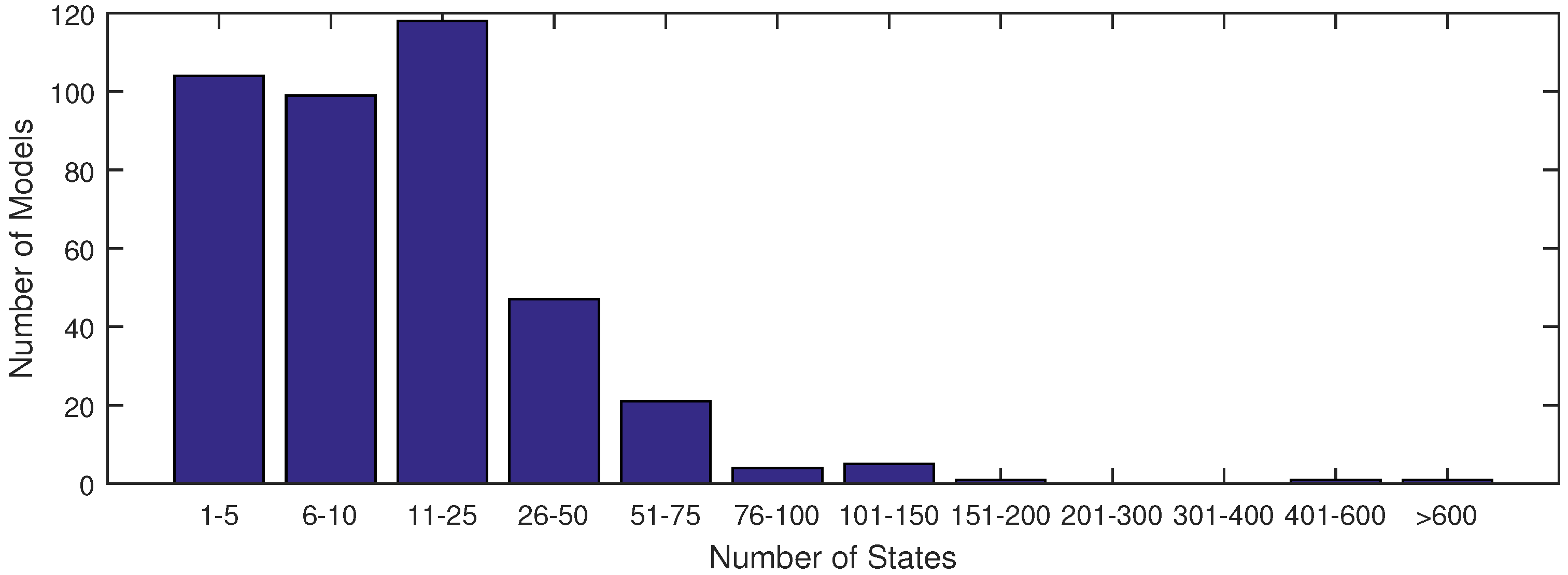
The majority of models used in systems biology today contain anywhere from 1 to 25 states (see Figure 1). This is largely due to the fact that anything beyond 25 states requires excessive computational time in order to achieve an acceptable fit of parameter estimates with current methods. With the increase in data availability and an emphasis on big data for drug testing, solvers must synthesize large datasets available from lab or clinical testing. A few researchers have already derived models to capture the dynamics of these large datasets, as found in [20,21], but reported large computational resource requirements. The objective of this work is to reduce development costs for large models by improving the parameter optimization to allow larger models and the incorporation of more data.

Figure 1. A distribution of model sizes according to number of states from the SBML database.

Figure 1. A distribution of model sizes according to number of states from the SBML database.

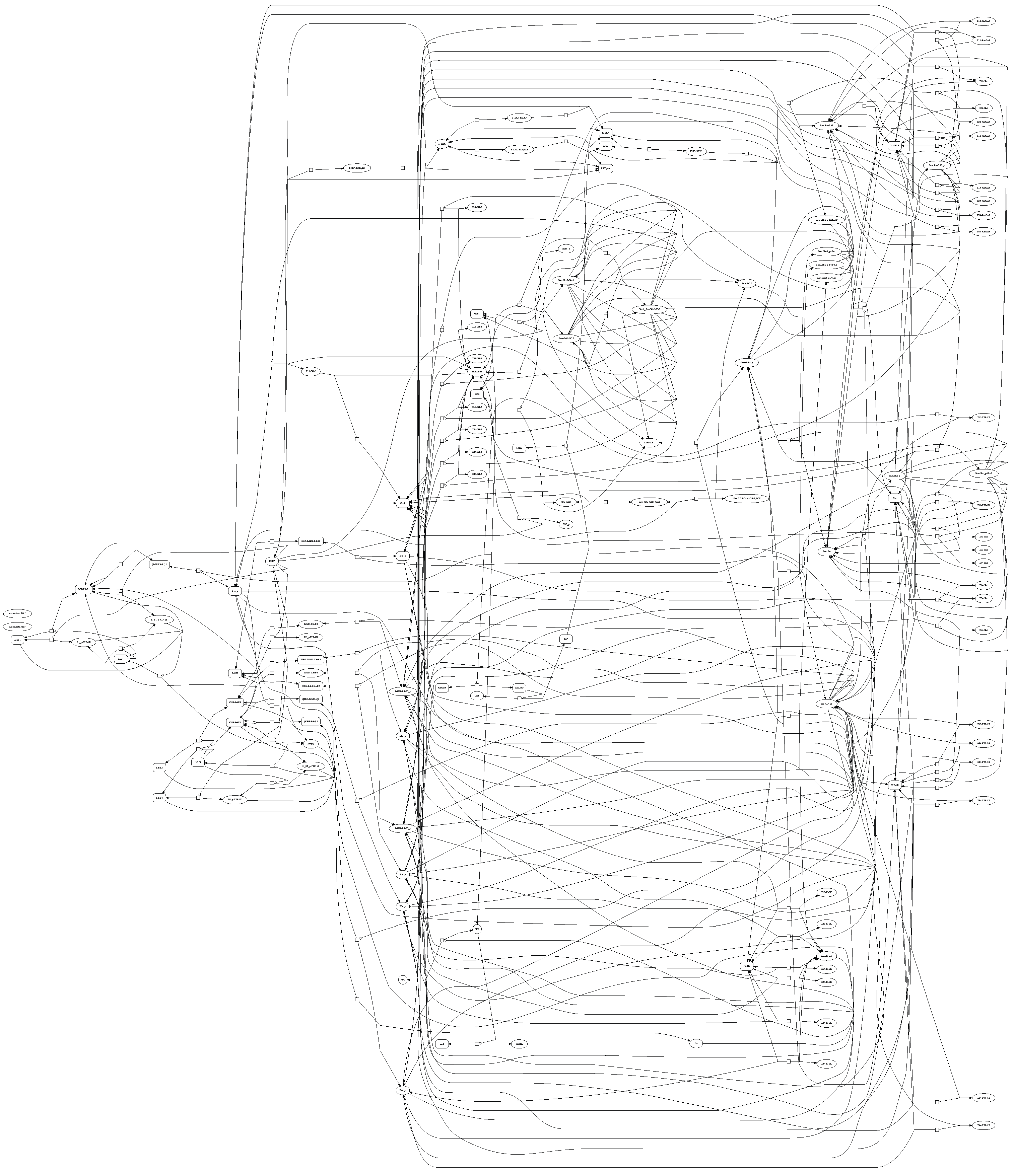
The ability of the proposed algorithms to estimate parameters is tested with one of the largest curated models from systems biology. The ErbB signaling pathway model is selected from the database of available curated SBML models as a benchmark problem. Figure 1 shows that there are very few models of comparable size to the ErbB model in the SBML database with a complex network of reactions as in Figure 2. The particular details of the ErbB model are not the focus of this work; instead, the model is used to demonstrate the proposed methodology for parameter estimation of large-scale and potentially over-parameterized models. Simulation and optimization methods have not yet advanced to allow larger models. Chen et al. [20] reported that a single parameter estimate required 24 h clock time on a 100-node cluster computer with the ErbB model.

When considering the size of the model, the sophistication and computational expense are tradeoffs that are carefully considered during the development process. Larger and more sophisticated models are often able to capture more details of the system, but at the expense of larger computational time and increased uncertainty due to over-parameterization. While the appropriate balance between sophistication and computation expense is not explored in this work, enabling larger models and more data synthesis with less computational expense reduces one of the major drawbacks of developing and using large-scale models.

Figure 2. ErbB signaling pathway through a network of reactions with rates that are proportional to individual reactant concentrations [22]. This reaction graph is a simpler version of the ErbB signaling pathway than Chen et al. [20] (used in this study) due to the impracticality of displaying a larger model.

Figure 2. ErbB signaling pathway through a network of reactions with rates that are proportional to individual reactant concentrations [22]. This reaction graph is a simpler version of the ErbB signaling pathway than Chen et al. [20] (used in this study) due to the impracticality of displaying a larger model.

1.1. Sequential Gradient-based Approaches

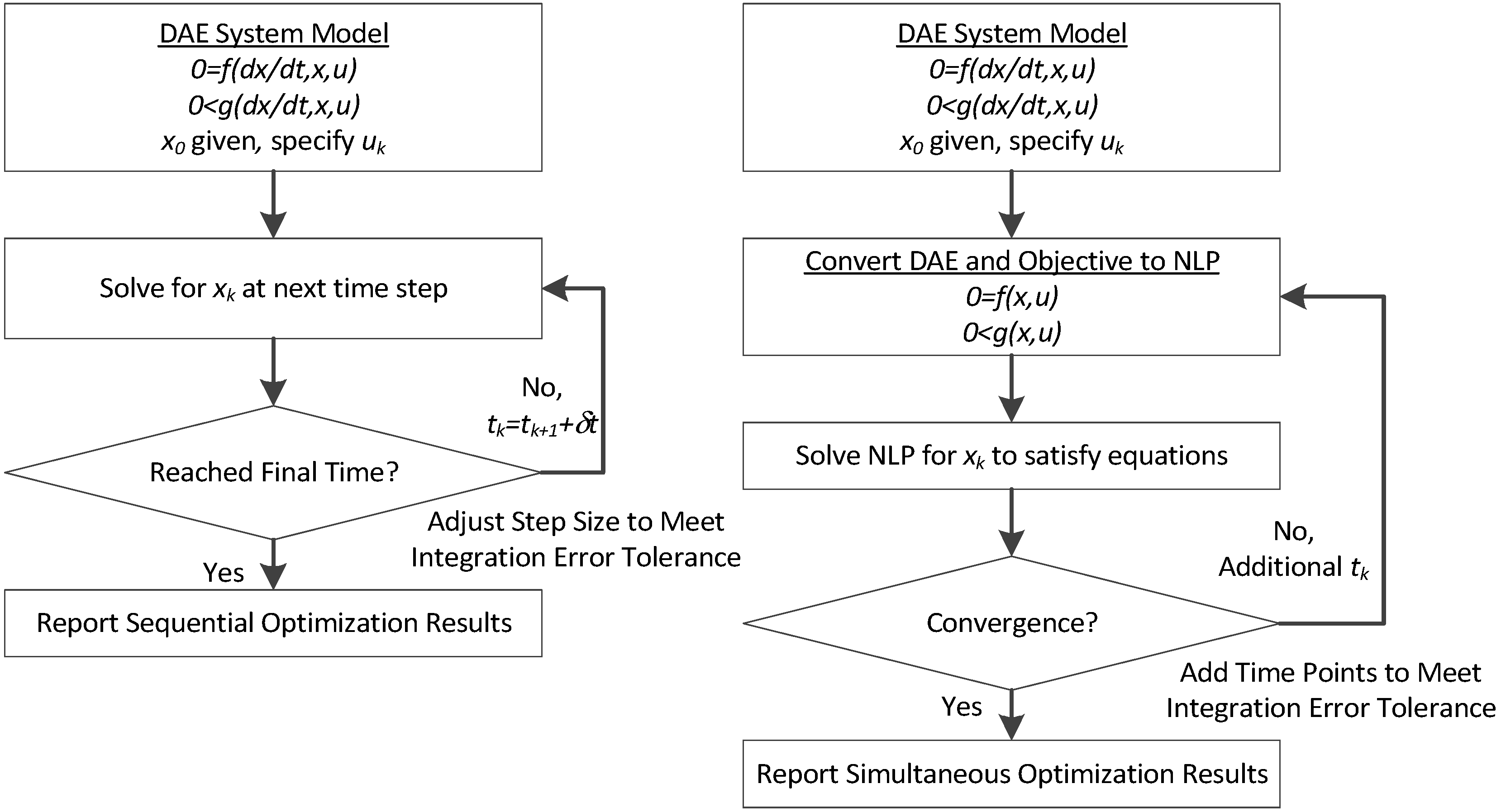
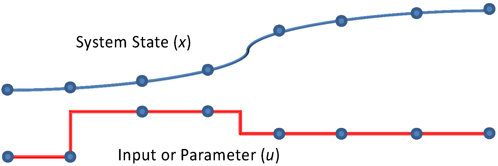
Gradient-based methods for parameter estimation can be separated into two groups as sequential and simultaneous strategies. In the sequential approach, also known as control vector parameterization, each iteration of the optimization problem requires the solution of the DAE model, and only the manipulated variables are discretized. In this formulation the manipulated variables are represented as piecewise polynomials [23,24,25], and optimization is performed with respect to the polynomial coefficients. Until the 1970s, these problems were solved using an indirect or variational approach, based on the first order necessary conditions for optimality obtained from Pontryagin’s Minimum Principle [26,27]. This approach takes a dynamical system from one state to the next based on given constraints to the system by minimizing the Hamiltonian over the set of all permissible controls. Often the state variables have specified initial conditions and the adjoint variables have final conditions; the resulting two-point boundary value problem (TPBVP) is addressed with different approaches, including single shooting, invariant embedding, multiple shooting or some discretization method such as orthogonal collocation on finite elements. A review of these approaches can be found in [28]. On the other hand, if the problem requires the handling of active inequality constraints, finding the correct switching structure as well as suitable initial guesses for state and adjoint variables is often very difficult. Early approaches to deal with these problems can be found in [27]. It has been established that sequential approaches have properties of single shooting methods and do not perform well with models that exhibit open loop instability [29,30]. Shooting methods may fail with unstable differential equations before the initial value problem can be fully integrated, despite good guess values [31].

An improvement over the single shooting methods is multiple shooting, which is a simultaneous approach that inherits many of the advantages of sequential approaches. It solves a boundary value problem by partitioning the time domain into smaller time elements and integrating the DAE models separately in each element [32,33,34,35]. The initial value problem is solved in each of the smaller time intervals.

1.2. Simultaneous Gradient-based Approaches

In the simultaneous approach, also known as direct transcription, both the state and control profiles are discretized in time using collocation of finite elements. This approach corresponds to a particular implicit Runge–Kutta method with high order accuracy and excellent stability properties. Also known as fully implicit Gauss forms, these methods are usually too computationally expensive (and rarely applied) as initial value problem solvers. However, for boundary value problems and optimal control problems, which require implicit solutions anyway, this discretization may be a less expensive way to obtain accurate solutions. On the other hand, the simultaneous approach leads to large-scale NLP problems that require efficient optimization strategies [16,17,36,37]. As a result, these methods directly couple the solution of the DAE system with the optimization problem; the DAE system is solved only once at the optimal point, and therefore can avoid intermediate solutions that may not exist or may require excessive computational effort.

Manipulated variables are discretized at the same level as the state variables. The Karush–Kuhn–Tucker (KKT) conditions of the simultaneous NLP are consistent with the optimality conditions of the discretized variational problem, and convergence rates can be shown under mild conditions [38,39,40]. More recently, these properties have been extended to Radau collocation. In Kameswaran and Biegler’s papers [41,42], convergence rates are derived that relate NLP solutions to the true solutions of the infinite dimensional optimal control problem.

Similar to multiple shooting approaches, simultaneous approaches can deal with instabilities that occur for a range of inputs. Because they can be seen as extensions of robust boundary value solvers, they are able to “pin down” unstable modes (or increasing modes in the forward direction). This characteristic has benefits in problems that include transitions to unstable points, optimization of chaotic systems [35] and systems with limit cycles and bifurcations, as illustrated in [30]. Simultaneous methods also allow the direct enforcement of state and controlled variable constraints, at the same level of discretization as the state variables of the DAE system. As discussed in Kameswaran and Biegler [42], these can present some interesting advantages on large-scale problems. Recent work [42,43,44] has shown that simultaneous approaches have distinct advantages for singular control problems and problems with high index path constraints.

The simultaneous approach has a number of advantages over other approaches to dynamic optimization. Betts [45] provides a detailed description of the simultaneous approach with full-space methods, along with mesh refinement strategies and case studies in mechanics and aerospace. Systems biology models may also be ill-conditioned and non-convex where many gradient-based local optimization methods fail to find global solutions. This obstacle has been overcome by methods involving deterministic and stochastic global optimization [46].

1.3. Parameter Optimization

A model for a biological system is necessary in order to evaluate parameters that are not as readily measured experimentally. Further, experimentation methods to evaluate all mechanism parameters are in many cases impractical, but fortunately current techniques allow for use of models to estimate unknown parameters [47]. It is important to ensure that there is the right structure in the model (observability) for parameter estimation and that the data contains sufficient information to produce correct parameter values. In the case of computational systems biology, the structure of the model typically indicates that a subset of the model parameters may not be uniquely estimated. In Chis et al. [18], a comparison of techniques for the selection of the parameter subset shows that the generating series approach in combination with an identifiability analysis is the most widely applicable strategy.

Another challenge in parameter estimation for systems biology is that the experimental data available for biological models is often noisy and taken at a limited number of time points. Lillacci and Khammash [48] proposes a method based on an extended Kalman filter (also known as a dynamic recursive estimator) to find valid estimates of model parameters and discriminate among alternative models of the same biological process. Word et al. [49] also discusses the capabilities of nonlinear programming and interior-point methods to efficiently estimate parameters in discrete-time models.

In the past, different approaches, including both simultaneous and sequential approaches, have been used for optimization of large-scale models, such as the genome-scale dynamic flux balance models studied in Leppävuori et al. [4]. A method is proposed for parameter estimation selection using both simultaneous and sequential approaches to optimize the model parameters. In the sequential estimation strategy with direct sensitivities, the authors conclude that “in this formulation, the size of the problem grows large with the genome-scale metabolic models, and would be outside the capabilities of today’s laptop hardware.”

Regarding parameter selection, Gutenkunst et al. [50] make the important distinction that modelers should focus on predictions rather than strictly on parameters. That is, even if individual parameters are poorly constrained, collective fitting of parameters can lead to well-constrained predictions. In many models, the available in vivo data means that the full set of parameters is often not uniquely identifiable. Thus, the model should be evaluated and reduced by fixing some parameters to literature values or properly grouping some sets of parameters. Rodriguez-Fernandez et al. [51] propose a method of doing this in a single step with a MINLP-based optimization approach.

Coelho et al. [52] discuss a general framework for uncertainty analysis in parameter estimation. Uncertainty analysis is beyond the scope of this paper because the major case study involves a model that already has optimal parameters, which are perturbed and it is left to the solver to return to the optimal solution. Nevertheless, in a typical parameter optimization case study in which the nominal values are not known, it would be an important consideration. Chung [53] proposes a sensitivity analysis for a distributed parameter estimation problem. This method results in improved parameter estimates. The idea of using sensitivity to determine parameter perturbations is one way to enhance the convergence of the ErbB model.

2. Simulation and Optimization of DAE Systems

A framework for simulation and parameter estimation in systems biology is developed to detail the novel strategy proposed for overcoming challenges with large-scale models and relatively few parameters. The framework is also applicable to other systems with relatively low degrees of freedom and large state dimensions.

2.1. Simulation of DAE Systems

One common form for mathematically describing dynamic systems is through the use of differential and algebraic equations (DAEs), which includes both equality and inequality constraints (see Equation (1)).

$$0=f\left(\frac{dx}{dt},x,u\right)$$

(1a)

$$0<g\left(\frac{dx}{dt},x,u\right)$$

(1b)

where x is a vector of states that may appear in differential or algebraic form, u is a vector of inputs, f is a set of equality constraints, and g is a set of inequality constraints. This DAE form is less restrictive than other forms that require special arrangement to fit into semi-explicit form $\left(\frac{dx}{dt}=f\left(x,u\right)\right)$, discrete form $\left(x[k+1]=f\left(x\left[k\right],u\left[k\right]\right)\right)$, or that only allow equality constraints but not inequality constraints (see Equation (1b)). Another potential restriction with prior work is that a solver may only be able to solve differential equations (Ordinary Differential Equations (ODEs)) but not coupled with algebraic equations. The solution of DAEs has a long history of computational techniques for efficient simulation of large-scale and complex systems. Two general approaches for simulation of DAEs are shown in Figure 3 with a sequential approach [54,55,56,57,58,59,60,61] shown on the left and a simultaneous approach [17,62,63,64,65,66,67,68,69,70,71] shown on the right.

Figure 3. Overview of sequential (left) and simultaneous (right) approaches to solve DAE systems.

Figure 3. Overview of sequential (left) and simultaneous (right) approaches to solve DAE systems.

For both approaches, the equations are solved as an initial value problem (IVP) where the initial states $\left(x_0\right)$ and decision variables $\left(u_{k\forall (1..N)}\right)$ over the time horizon are specified as seen in Figure 4, in which N is the number of time steps in the discretized horizon.

Figure 4. DAEs are discretized and solved over a time horizon with System States (x) determined from the equations and Inputs or Parameters (u) that may discontinuously adjust at points in the simulated time horizon.

Figure 4. DAEs are discretized and solved over a time horizon with System States (x) determined from the equations and Inputs or Parameters (u) that may discontinuously adjust at points in the simulated time horizon.

There is no objective function to drive variables to a best case value and the presence of inequality constraints may allow multiple feasible solutions. If there are no inequality constraints but only equality constraints, then the simulation requires an equal number of equations and variables to be completely specified. In the case where there are more independent equations than variables, the system is described as over-specified and a solution may not exist that can satisfy all equations. In the case where there are more variables than equations and active inequality or equality constraints, the system is described as under-specified or with additional degrees of freedom. In this case, additional variables can be specified, otherwise those variables can be selected by an optimizer to minimize a particular objective.

An advantage of solving DAEs with a sequential method is that the solution is a series of smaller IVPs as compared with one large IVP with a simultaneous approach. In the sequential approach, the time step is adjusted either smaller to achieve greater accuracy or larger to speed up computational time. With a simultaneous approach, the DAE system is discretized before the solution and converted to a Nonlinear Programming (NLP) problem for solution by a large-scale iterative solver. The simultaneous approach converges all variables and equations in the time horizon with one call to the solver. If the solution does not meet integration accuracy requirements, the grid is refined and another solution is attempted. The later approach may be advantageous when there is a need to trade off certain variables or parameters that are calculated or fixed. With a simultaneous approach, any point along the time horizon can be specified or fixed as long as another variable is given to the optimizer to adjust. For example, a final value for a particular variable could be fixed if the initial condition is calculated.

2.2. Optimization of DAE Systems

When there are additional degrees of freedom, such as unknown parameters in dynamic data reconciliation or a manipulated variable move plan in Model Predictive Control (MPC), an objective function J can be defined to drive the selection of those variables (see Equation (2)).

$$\underset{u,x}{min}J\left(x,u\right)$$

(2a)

$$0=f\left(\frac{dx}{dt},x,u\right)$$

(2b)

$$0\le g\left(\frac{dx}{dt},x,u\right)$$

(2c)

where the objective function $J\left(x,u\right)$ is minimized by adjusting the state vector x and the vector of decision variables u. The same set of equality (f) and inequality (g) constraints are present as described in Section 2.1. The numerical solution of Equation (2) is more challenging than the simulation case of Equation (1) because there may be many feasible values of x and u that must also minimize the objective. When there are few decision variables, an approach may be to try all combinations of decision variables to locate those that satisfy both constraints and then select the combination that produces the lowest objective. This direct search method is rarely applied in practice because of the number of trial points for u that must be computed grows quickly as the dimension of u increases. Two popular methods for optimizing systems of DAEs are again the simultaneous and sequential methods (see Figure 5).

The core of the sequential approach on the left of Figure 5 is the same as in Figure 3 where forward-propagation solvers are used to compute $x_k$ with $u_k$ fixed at specified values that are either provided by an initial guess or otherwise updated by the secondary loop. This secondary optimization loop computes several candidate solutions and gradients of those solutions while updating the guess value for $u_k$. This cycle continues until convergence criteria are met to ensure that Karush–Kuhn–Tucker (KKT) conditions for optimality are satisfied. The simultaneous approach on the right side of Figure 5 includes the objective and constraints in a single solution attempt to simultaneously converge the equations and minimize the objective function. This is accomplished by transforming the DAE into NLP form and adding the standard objective function for NLP solvers. Some refinement of the grid structure may be necessary to reduce integration error and satisfy accuracy requirements. Terminating the solver before convergence is achieved does not typically result in a feasible solution to f and g because it is only at the converged solution that a feasible solution is computed. On the other hand, if the sequential solution approach is terminated after a specified number of iterations, a sub-optimal but feasible solution exists.

Figure 5. Overview of sequential (left) and simultaneous (right) approaches to optimize DAE systems.

Figure 5. Overview of sequential (left) and simultaneous (right) approaches to optimize DAE systems.

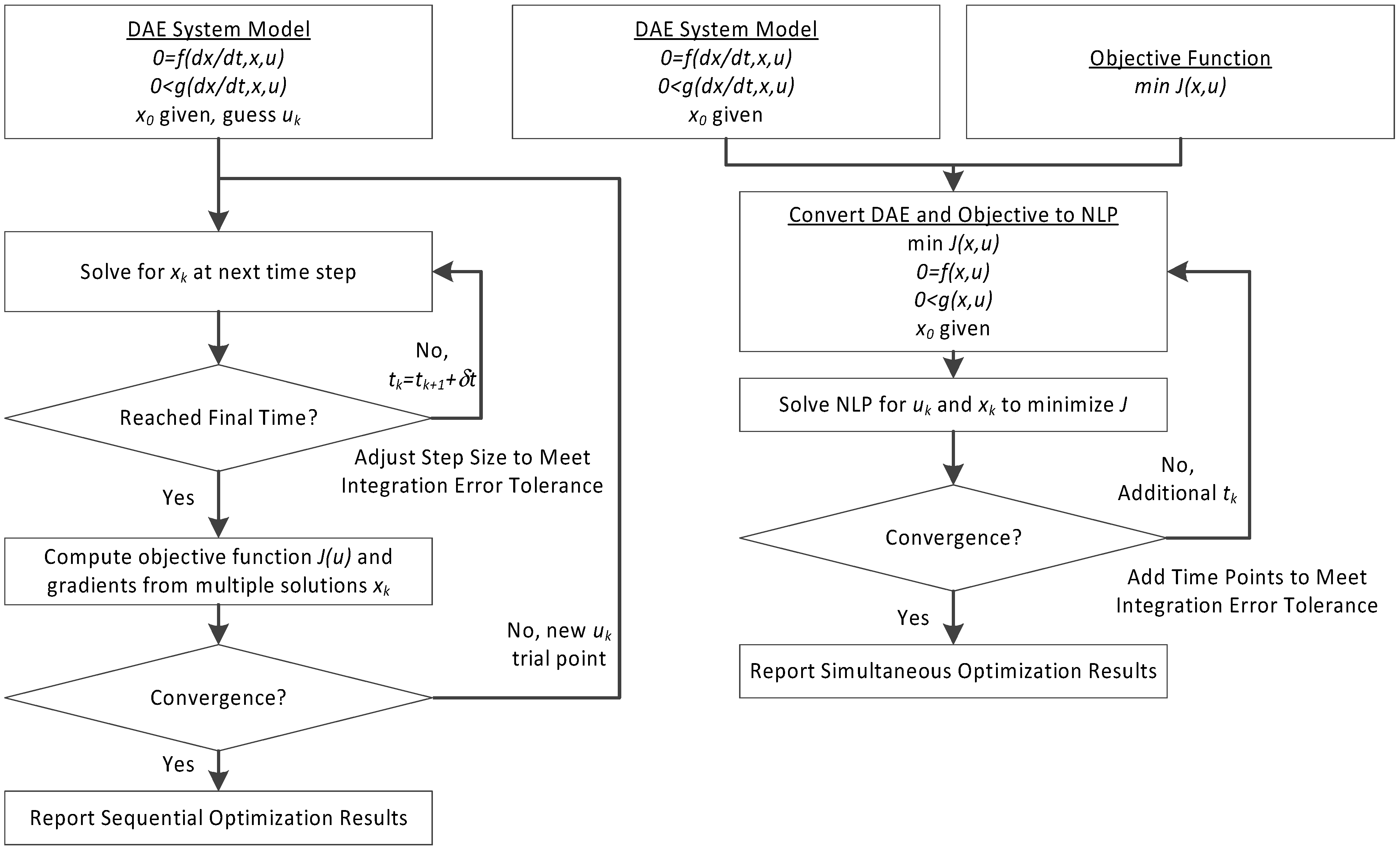
3. Hybrid Simultaneous and Sequential DAE Optimization

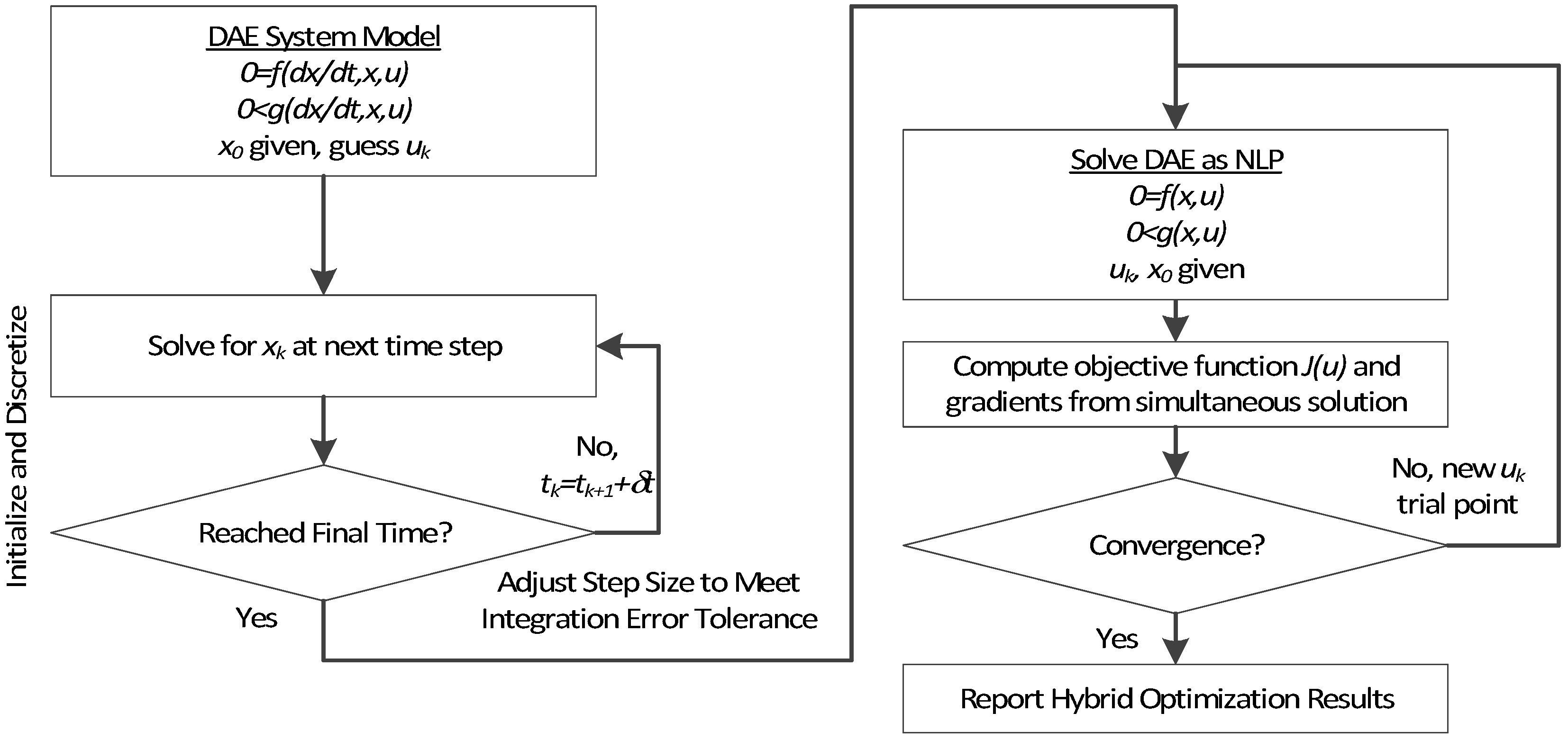
This section details the hybrid approach that combines a simultaneous and sequential approach to improve convergence speed and reliability (see Figure 6).

Figure 6. Overview of the hybrid approach to initialize and optimize DAE systems with initialization on the left followed by optimization on the right.

Figure 6. Overview of the hybrid approach to initialize and optimize DAE systems with initialization on the left followed by optimization on the right.

The method is a hybrid method in two ways, including (1) initialization and discretization that occurs before the model is converted from DAE to NLP form, and (2) a simultaneous core solution with no degrees of freedom in a loop with efficient sensitivity and gradient calculations. The first step for initialization is accomplished with a sequential approach to adjust the step size with guess values for $u_k$. The optimal discretization is likely to change with changing $u_k$ values produced by the optimization, but this may be a better method than heuristic discretization methods. The second step is the optimization loop, which uses a simultaneous simulation to provide a search direction for $u_k$. The calculation of a search direction from the simultaneous simulation is a post-processing solution step and is more efficient than solving additional adjoint equations often augmented to a sequential solution approach.

Gradient-based sequential solutions require derivative information of the objective sensitivity with respect to the adjustable parameters to determine a search direction that improves the objective. A new search direction is selected with the Newton–Raphson method. This method determines a change in parameters $\left(du\right)$ that satisfies the Karush–Kuhn–Tucker (KKT) optimality conditions (Equation (3a)) with Lagrange multipliers for the lower $\left({\lambda }_{i\forall (1..p)}\right)$ and upper $\left({\lambda }_{i\forall (p+1..2p)}\right)$ bounds for u. The gradient is approximated with a Taylor series approximation (Equation (3b)) with the first and second derivatives of the objective. A search direction is calculated by inverting the second derivative matrix (see Equation (3c)) as implemented in the APMonitor Modeling Language and Optimization Suite [72].

$${\nabla }_{u}J(\overline{u}+du)-\sum _{i=1}^p{\lambda }_i\left(a-u\right)-\sum _{i=1}^p{\lambda }_{i+p}\left(u-b\right)=0$$

(3a)

$${\nabla }_{u}J(\overline{u}+du)\approx {\nabla }_{u}J\left(\overline{u}\right)+{\nabla }_{uu}^{2}J\left(\overline{u}\right)du$$

(3b)

$$du=-{\left({\nabla }_{uu}^{2}J\left(\overline{u}\right)du\right)}^{-1}{\nabla }_{u}J\left(\overline{u}\right)$$

(3c)

Accurate first (Jacobian) and second (Hessian) derivatives improve the search direction but can be computationally expensive to obtain. The most computationally expensive option is to use finite difference methods where $p+1$ separate simulations are performed with small perturbations in the parameter value of $u_{i\forall (1..p)}$. Second derivative approximations may be obtained with $p^2+p$ additional numerical integrations, but this is not typically performed due to increased computational burden. Without a suitable Hessian approximation, the method becomes a steepest descent algorithm where the Hessian is set as the identity matrix with a search direction of $du=-{\nabla }_{u}J\left(\overline{u}\right)$. Several approximate methods exist to obtain an approximate Hessian solely from Jacobian information. One such method is a quasi-Newton approach where a rank-1 BFGS update maintains a positive definite Hessian or an inverted Hessian approximation. This methods starts as a steepest descent algorithm and then transitions to a Newton–Raphson approach as the Hessian information is obtained.

Instead of finite difference methods, accurate first derivatives $\left({\nabla }_{u}J\left(\overline{u}\right)\right)$ can be obtained by solving adjoint sensitivity equations [73,74,75]. The cost is the additional computational expense and configuration to solve additional equations at every time step. Without exact Hessian information, a quasi-Newton approach can be used to converge more rapidly than the steepest descent method.

A third method to obtain accurate derivative information is a post-processing step to a simultaneous time-discretized solution. Time discretization is performed with orthogonal collocation on finite elements [76] for solution by nonlinear programming (NLP) or mixed integer nonlinear programming (MINLP) solvers. This method is fast because it only involves a sparse matrix inversion as a post-processing step to a single dynamic simulation. Exact derivatives to machine precision are available through automatic differentiation for equation gradients with respect to states $\left(\nabla f_x(x,u)\right)$ and parameters $\left(\nabla f_u(x,u)\right)$, and for objective gradients with respect to states $\left(\nabla J_x(x,u)\right)$ and parameters $\left(\nabla J_u(x,u)\right)$. Note that $\nabla J_u(x,u)$ is not the same as $\nabla J_u\left(u\right)$. In the case of $\nabla J_u\left(u\right)$, there is no state x dependence because the states are deemed as implicit functions of u. The sensitivities are determined by solving the following set of linear equations at the solution of the dynamic simulation with parameter current guess $\overline{u}$ and corresponding state solution $\overline{x}$ (see Equation (4)).

$$\left[\begin{array}{ccc}{\nabla }_{x}f(\overline{x},\overline{u})& {\nabla }_{u}f(\overline{x},\overline{u})& \mathit{0}\\ {\nabla }_{x}J(x,u)& {\nabla }_{u}J(x,u)& -\mathit{1}\\ \mathit{0}& I& \mathit{0}\end{array}\right]\left[\begin{array}{c}{\nabla }_{u}x\\ {\nabla }_{u}u\\ {\nabla }_{u}J\left(\overline{u}\right)\end{array}\right]=\left[\begin{array}{c}\mathit{0}\\ d{u}_i=1\\ \mathit{0}\end{array}\right]$$

(4)

An efficient implementation of this calculation involves obtaining a Lower Upper (LU) factorization of the left hand side (LHS) mass matrix. The linear system of equations is successively solved for the different right hand side (RHS) vector where the row corresponding to $d{u}_i$ is set equal to 1 and all other elements are set equal to 0. The solution produces the sensitivity of the states with respect to the parameters at every time point in the horizon $\left({\nabla }_{u}x\right)$ as well as the sensitivity of the objective with respect to the parameters $\left({\nabla }_{u}J\left(\overline{u}\right)\right)$. The Hessian of the objective with respect to the parameters is then calculated with Equation (5).

$${\nabla }_{uu}^{2}J\left(\overline{u}\right)={\nabla }_u{x}^T{\nabla }_{xx}J(\overline{x},\overline{u}){\nabla }_{u}x$$

(5)

This calculation also relies on the Hessian of the objective with respect to the states $\left({\nabla }_{xx}J(\overline{x},\overline{u})\right)$ that is available at the solution with the use of automatic differentiation.

In summary, a new hybrid dynamic optimization method is proposed that solves a simultaneous simulation in the inner loop and a sequential optimization for the outer loop. The proposed hybrid method combines the simultaneous solution and sensitivity calculation that have high computational efficiency with the lower-dimensional sequential approach that has only parameters as decision variables. This combination is shown to perform nearly as fast as the fully simultaneous approach where parameters and model states are calculated together. The method also provides updated parameters at every cycle of the outer loop sequential iterations in case early termination or convergence monitoring is desired.

3.1. Model Parameter Estimation with HIV Case Study

A common benchmark model and simulation results are used to verify the proposed approach with literature values. The model used is a basic model describing dynamics of healthy, infected, and virus infected cells over thirty days with nine parameters, three variables, and three differential equations (see Equations (6a)–(6c)) [77]. An additional algebraic equation (see Equation (6d)) is added to scale the virus response as it changes by many orders of magnitude. The proposed algorithm successfully replicates the results published in literature and simulations in MATLAB. While the HIV model is a simple dynamic model with only four states, it is useful for demonstrating the proposed approach to much more complicated systems of equations. The full source code for this example is provided online [78].

The initialization strategy is applied to a parameter estimation problem in systems biology similar to the approach taken in [79]. In this case, a dynamic response of the spread of the virus is predicted and aligned with virus count data. The simulation predicts a count of the healthy cells (H), infected cells (I), and virus (V) in a patient. The $lo{g}_{10}$ value of the virus is fit to data with a least squares objective with six parameters $\left(k{r}_{i\in \left(1..6\right)}\right)$.

$$\frac{dH}{dt}=k{r}_1-k{r}_{2}H-k{r}_{3}HV$$

(6a)

$$\frac{dI}{dt}=k{r}_{3}HV-k{r}_{4}I$$

(6b)

$$\frac{dV}{dt}=-k{r}_{3}HV-k{r}_{5}V+k{r}_{6}I$$

(6c)

$$V_L=lo{g}_{10}V$$

(6d)

The parameter $k{r}_1$ is the natural rate of healthy cell generation per year. The parameters $k{r}_2$, $k{r}_4$, and $k{r}_5$ are the fractional death rate of healthy cells (H), infected cells (I), and virus count (V), respectively, on an annual basis. The parameter $k{r}_3$ is the rate constant for healthy cells becoming infected cells. An infection of a healthy cell reduces the healthy cell count and consumes a virus while increasing the infected cell count ($H+V\stackrel{k{r}_3}{\to }I$). The rate constant is multiplied by the number of healthy cells and virus count as each of those quantities affects the rate of infection. Infected cells have a higher death rate than healthy cells ($k{r}_4>k{r}_2$) in this model. Virus production depends on the parameter $k{r}_6$ and the number of infected cells.

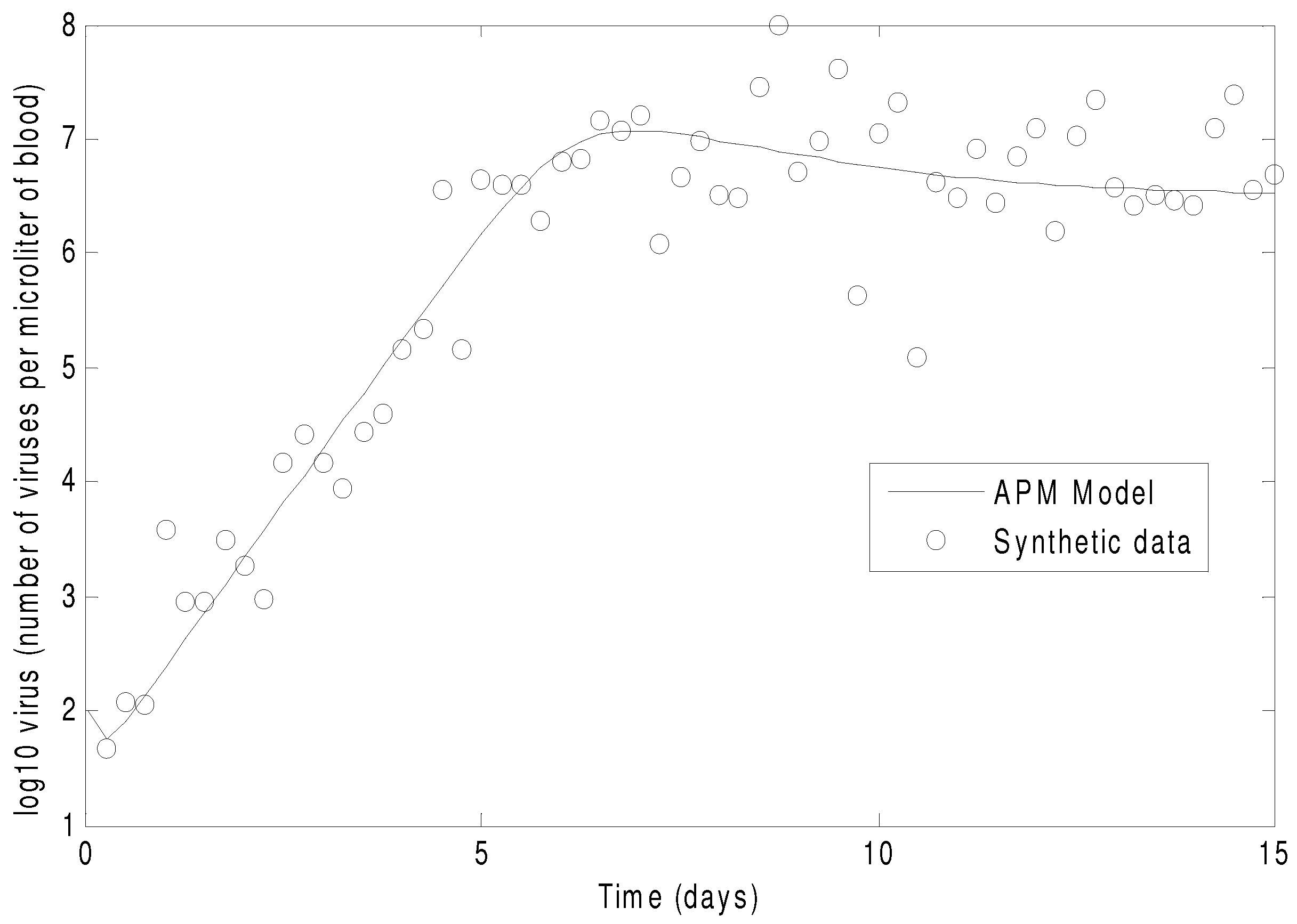
The simultaneous algorithm is consistent with sequential methods that include error control. A next step is to verify the parameter estimation capabilities with the benchmark problem. In order to perform the parameter estimation, the objective function is set to minimize the absolute error between the model and synthetic data. An arbitrary measurement noise of $\pm 0.5$ log order is added to the synthetic data. All six parameters values are perturbed by 10% from the optimal values to determine whether the proposed algorithm can find the correct parameter values from several different starting points. It is found that the simultaneous method is able to accurately optimize to the correct parameter values. Figure 7 shows the concentration of the virus from the synthetic data and the predicted model values with the estimated parameters. As seen in the figure, the simultaneous method is able to correctly find the parameters that allow the model to fit the synthetic data. The initialization is accomplished in two steps with the dynamic decomposition solution in lower block triangular form (0.7 s) followed by simultaneous (29 iterations in 1.1 s) or sequential dynamic parameter estimation (4 iterations in 2.1 s). The dynamic optimization problems of 843 variables and 840 equations are solved in APMonitor (APOPT solver) on a 2.4 GHz Intel i7-2760QM Processor. The APOPT solver fails to find a solution when initialization is not used. The decomposition successfully initializes the dynamic optimization problem by providing a nearby solution that is sufficiently close to the optimized solution. The optimized solution is shown in Figure 8 on a semi-log scale plot.

Figure 7. The parameters of the HIV model are adjusted to fit synthetic virus concentrations from simulated lab data.

Figure 7. The parameters of the HIV model are adjusted to fit synthetic virus concentrations from simulated lab data.

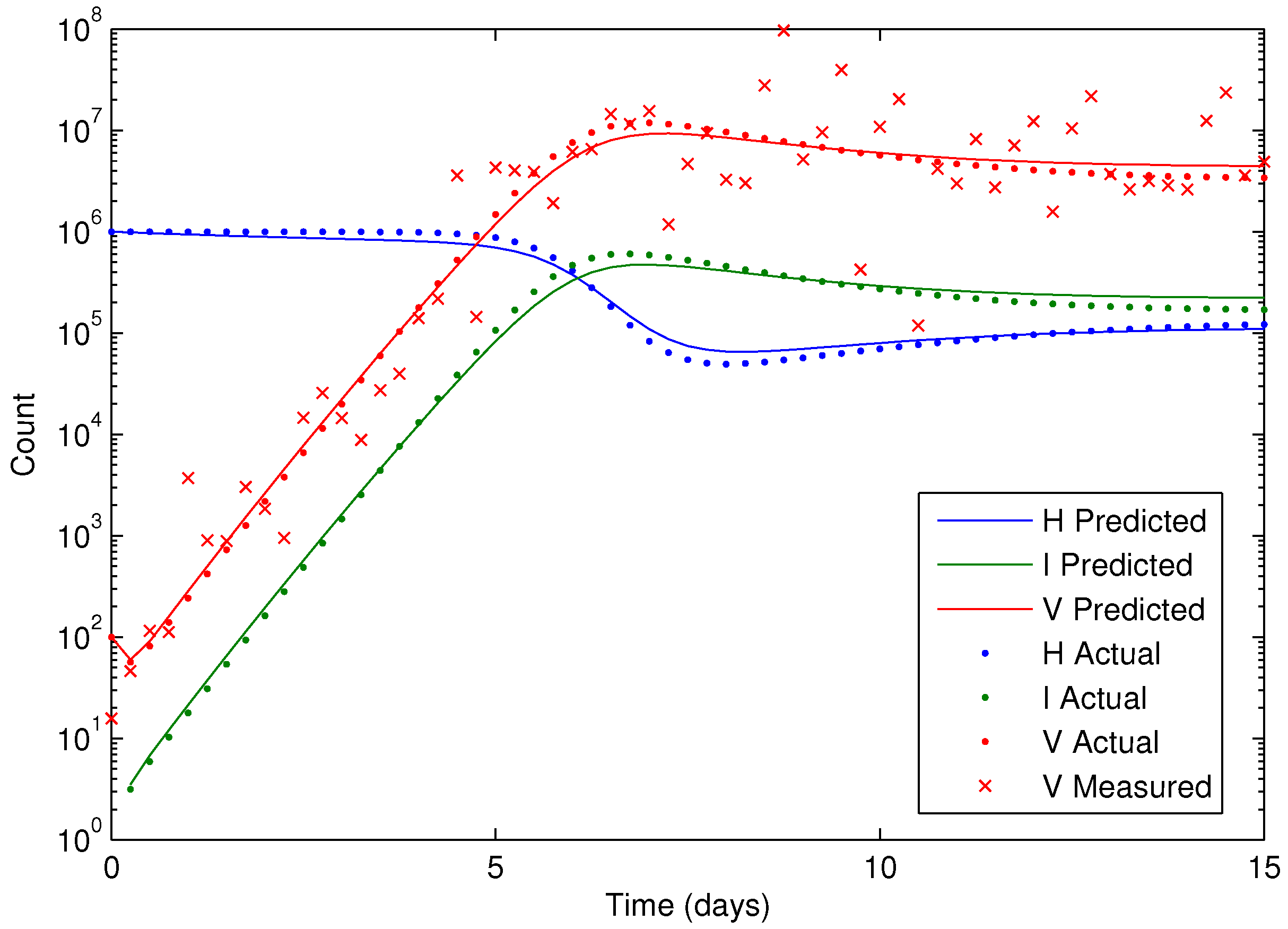
Figure 8. Results of the HIV model parameter estimation, including predicted, actual, and measured virus (V), infected cells (I), and healthy cells (H).

Figure 8. Results of the HIV model parameter estimation, including predicted, actual, and measured virus (V), infected cells (I), and healthy cells (H).

The discretized dynamic simulation is not successful without initialization, so the lower block triangular form of the sparsity is used to identify small subsets that can be solved successively and independently (see Figure 9). Although the DAE model has only four variables and equations, the optimization problem has over 800 variables and equations when it is discretized in time. A dot in Figure 9 indicates that the particular variable is present in that particular equation. For example, variable 402 is in equations 401–404. Each of the four variables of Equation (6) is solved at each time point in the horizon. These are the variables and equations along the diagonal on the left subplot of Figure 9. The zoomed-in view of variables and equations 400–420 shows repeated clusters of four variables and equations, which are the DAE model at each point in the time horizon. The upper right diagonal of that same subplot shows a zoomed-in view of variables 200–220 and equations 630–650, which are the non-differential variables $\left(H,I,V,V_L\right)$ in the collocation equations that relate derivative terms to non-derivative terms. The lower diagonal elements are the differential terms $\frac{dH}{dt}$, $\frac{dI}{dt}$, and $\frac{dV}{dt}$ in the collocation equations. The right subplot of Figure 9 shows the rearranged sparsity pattern with blocks of variables and equations that are solved successively and independently for the purpose of initialization. Full details on the decomposition and initialization method for DAEs are given in a related work [80].

Figure 9. Lower block triangular form with blocks of variables and equations that are solved successively and independently.

Figure 9. Lower block triangular form with blocks of variables and equations that are solved successively and independently.

Before this method of parameter estimation is applied to large-scale biological models, it is necessary to create an automatic conversion from SBML to an APMonitor form of the model. This not only eliminates the human error in the conversion process but also allows for the quick evaluation of many publicly available models. The converter is available at the following reference [81]. This conversion tool is used to automatically convert the model that describes the ErbB signaling pathways [20], referred to as the ErbB model, to demonstrate further capabilities with large-scale systems.

3.2. Systems Biology: ErbB Signaling Pathway Model Parameter Estimation

The ErbB signaling pathway (referred to henceforth as the ErbB model) is particularly important to understand and model for the purpose of pharmaceutical development. There are currently a wide variety of anti-ErbB drugs in use or development [20]. These are significant because it has been shown that a loss of signaling by any member of the ErbB protein family can result in embryonic lethality, while excessive ErbB signaling can result in the development of a variety of cancers [82,83]. Thus it is important to understand and model this pathway to ensure appropriate amount of ErbB signaling to reduce side effects. The ErbB model serves as a test case for this study of a large-scale model that is challenging to solve for parameter estimation. The references cited in this paper give additional details and innovations with the ErbB model. The focus of this work is a framework to numerically optimize large-scale systems biology models. Like the HIV example case, full source code for this example problem is also provided online [78].

The ErbB model has been the subject of several key studies in the field of computational biology [84]. Anderson et al. [84] develop tools that are used to produce biologically meaningful, simplified models from large-scale models, using the ErbB model as a case study. The purpose of using the ErbB model in this study is to show the ability of the proposed methods to decrease computational time required to obtain a good fit to data in a large systems biology model.

The ErbB model is a large model with 225 parameters, 504 variables and 1331 DAEs describing the kinetics of the signaling pathway. In the article, the authors estimated 75 of the initial conditions and rate constants out of the 229 identified by the sensitivity analysis. This is accomplished through simulated annealing, which required 100 annealing runs and 24 h on a 100-node cluster computer on average to obtain just one good fit. This constitutes a very large model in computational biology, as discussed above (see Figure 1). In this figure, the ErbB model is in an upper category at 525 states.

3.2.1. Improved Convergence through Model Transformation

To increase the likelihood of successful convergence for the model, it is desirable to have less nonlinearity in the model. In this example a logarithmic scale of model parameters is implemented. The ErbB model parameters vary across a large range of about fifteen orders of magnitude. The $lo{g}_{10}$ scaling provides a means to optimize the parameters without the inconsistencies in magnitude of perturbation. For example, a near zero-valued parameter that is perturbed by a value of one changes significantly, while that same perturbation of one causes a negligible change in parameter value for large-valued parameters. For the log scaling of these models, parameters that are originally zero-valued are kept at a value of zero, given that $lo{g}_{10}\left(0\right)$ is undefined. The model parameters that involve the step function are kept at their original values because they are not selected for optimization and are treated as known values. In addition, most of these step function parameters are zero-valued in one segment of the time horizon and then later turned on, becoming non-zero-valued. For future reference, another method of logarithmic scaling to handle zero-valued parameters would be to scale them as $lo{g}_{10}(\theta +1)$ so that the parameters are still valued at zero in the corresponding times, while being adjusted accordingly at other times. Although this would cause some problems with perturbations, the key aspect of the logarithmic scaling is consistency.

Although logarithmic scaling is implemented in this specific example, any model transformation that improves the linearity of input/output relationships has the potential to improve model convergence. In some cases, such as this, model transformation is necessary to achieve successful convergence. Otherwise the solver fails to find a solution within a maximum allowable time limit or maximum number of iterations.

3.2.2. Solver Performance on 341 Benchmark Problems

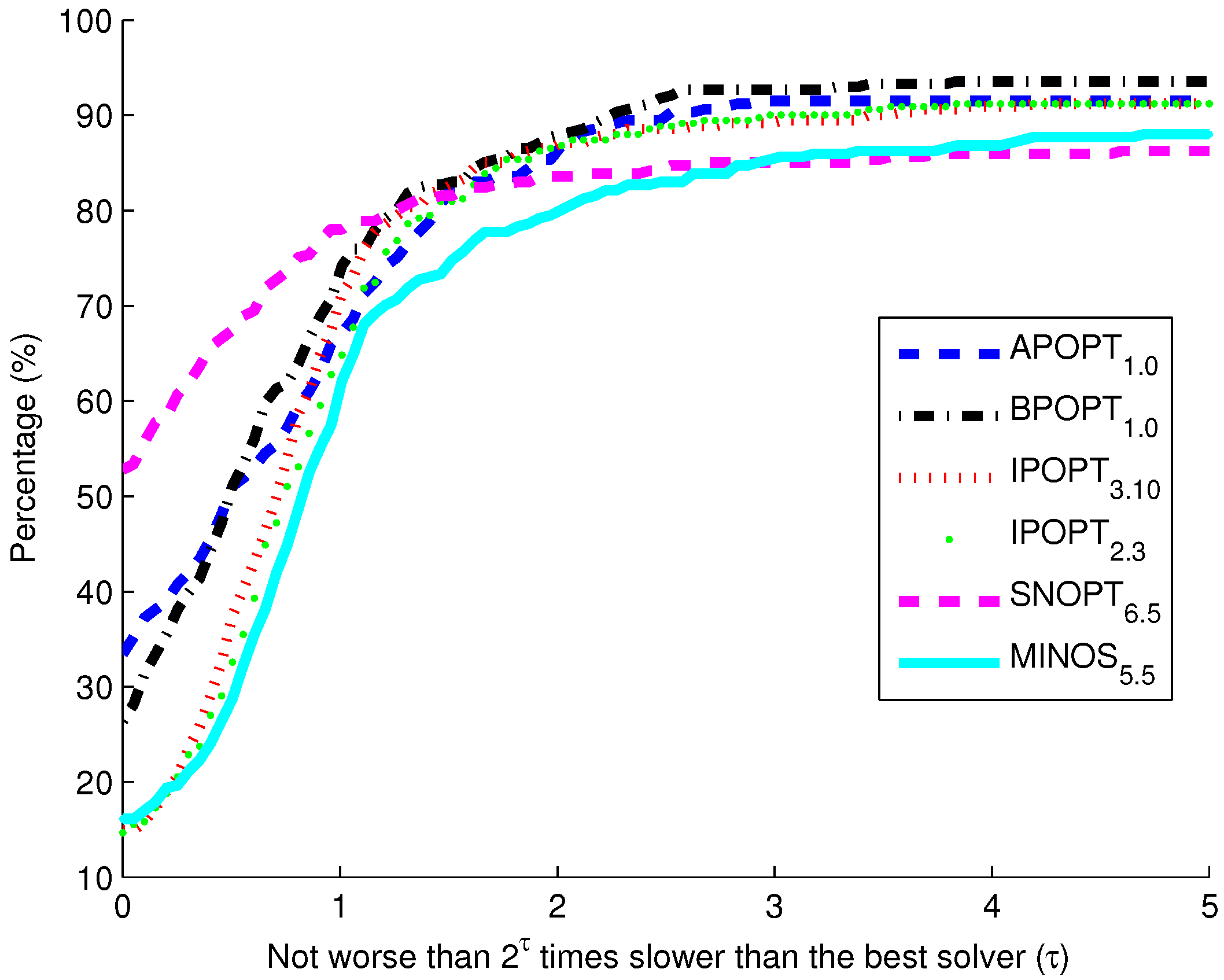
With the large-scale model problem, the choice of solver also proved to be a critical decision. A benchmark on the CPU times required for solution of 341 SBML models is performed for Nonlinear Programming (NLP) solvers APOPT [85], BPOPT, IPOPT [86], SNOPT [87], and MINOS that employ sequential quadratic programming (SQP). The results are shown in Figure 10. The benchmark indicates that the highest percentage of models solve successfully with BPOPT (interior point SQP method). The solver SNOPT (active set SQP method) has the shortest solution times for a large fraction of the models. This benchmark study points to a number of characteristics of interior point and active set methods for solving large-scale and sparse systems of differential and algebraic equations.

Figure 10. Benchmark solver results for biological models comparing six solvers over 341 curated models from the biomodels database.

Figure 10. Benchmark solver results for biological models comparing six solvers over 341 curated models from the biomodels database.

The purpose of these benchmark results is to show the speed of different popular solvers and the total number of problems that each can solve if given unlimited time. Only two examples are presented in detail in this paper. The benchmark results across 341 models give a broader view of potential applications in systems biology. The intercept shows that the solver SNOPT is fastest or tied for fastest on 52% of the set of 341 models. Other notable solvers include APOPT that is fastest or tied on 33% and BPOPT on 27% of the problems. IPOPT and MINOS are fastest or tied on 16%. Although SNOPT is a fast solver, it is least capable at finding a solution given additional time and solves only 86.2% of the problems when given $\tau =5$ or $2^5$ more time than the fastest solver. Notable solvers for convergence success include BPOPT at 93.5% and APOPT at 91.5% success rates. It is important to have a solver that can complete the solution quickly and with a high final success rate. Researchers often try multiple solvers when attempting challenging problems. These benchmark results show several promising solvers over a range of systems biology problems.

3.2.3. Unobservable Parameters

A common scenario is when certain parameters in a model have no or little influence on the predictions of the measured data. Those parameters cannot be estimated from available data because there is no information in the measurements to guide the selection of those parameters. For linear systems, an observability analysis is a common method to determine how many parameters can be estimated. Another approach is to simply leave insensitive parameters at default values by including a small penalty for all parameter value movement. A small cost function is included in the objective function for the possibility that the objective function is insensitive to the unknown parameter. This prevents the solver from moving the parameter to a random number if there is no objective function gradient with respect to the parameter. The cost function is added to the objective in the form $k{(\theta -{\theta }_0)}^2$ where k is a constant, θ is the parameter to be optimized, and ${\theta }_0$ is the initial value of that parameter (not the optimal value). By default k is set to a small value at ${10}^{-3}$ to not interfere with the primary objective of fitting model predictions to measured values.

3.3. Results of ErbB Parameter Optimization

The objective function minimizes the squared error between the model and two measurable concentrations, referred to as pAkt and pERK. Instead of using simulated annealing to estimate the parameters, a multi-start optimization is used. To accomplish this, the method first initializes the problem by receiving the input of a time horizon of parameters, the majority of which are subject to the indicator variables. This step returns the results of the simulation with the initial optimal parameters given by the model. The parameter values are then randomly varied from $\pm 1.0$ log order from the prior value. However, to receive consistent results between test runs, it is determined to vary the parameters randomly as $\pm 1/\left(sensitivity\right)$. The solver is then utilized to determine if a parameter optimization could return an acceptable fit with the available measurements. The model is highly constrained with little flexibility in order to return the optimal solutions. Without the log scaling or other initialization factors added to the model, the results are limited to the estimation of only a few parameters at a time. The estimation procedure is performed in APMonitor through MATLAB, Julia, or Python programming environment.

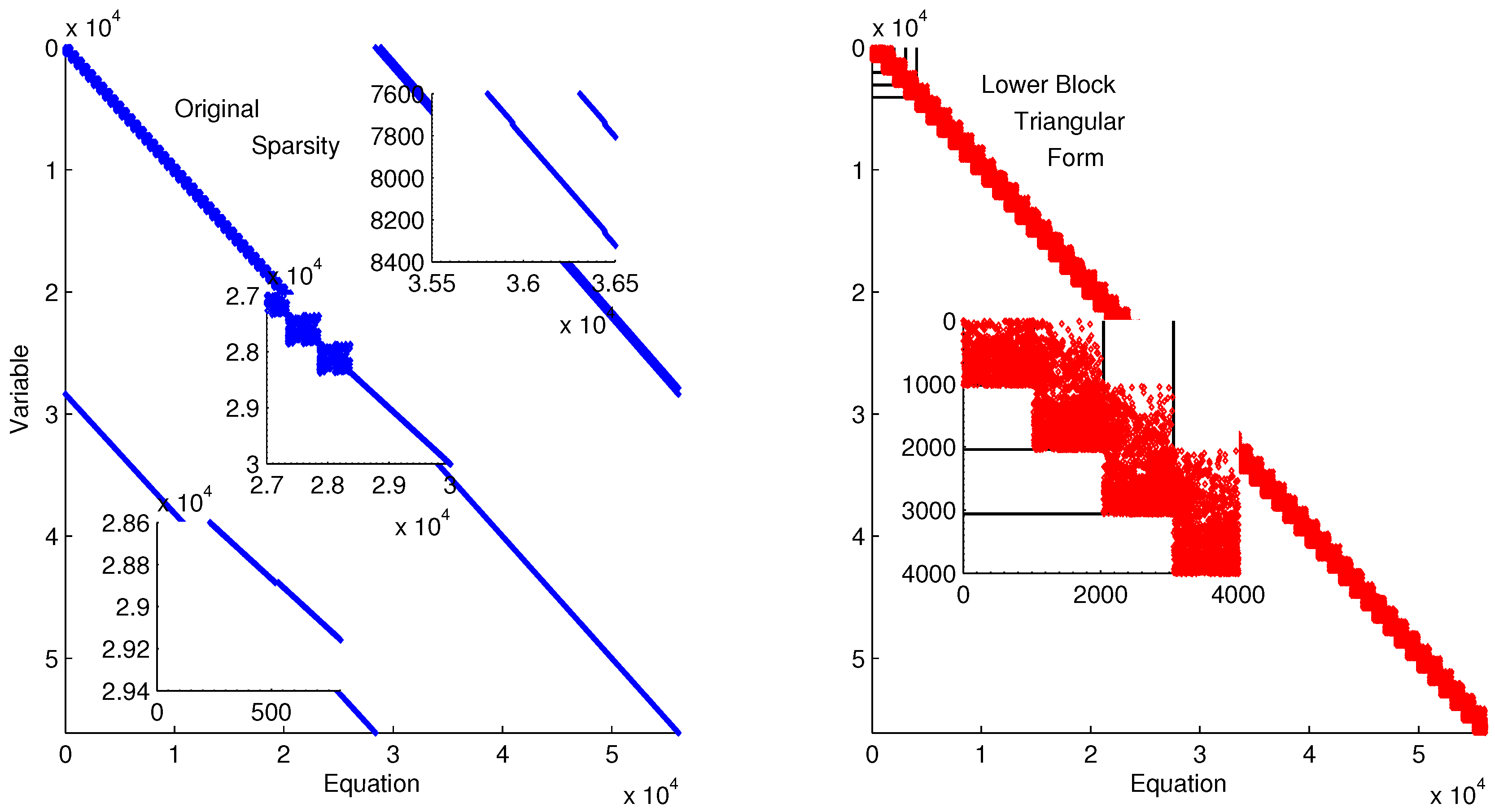
Figure 11 shows the lower block triangular form of the ErbB model for improved initialization of the parameter optimization. Transforming into lower block triangular form also decomposes the problem into a simpler form for solution. In this decomposition, the structure of the time-discretized model is detailed to expose sets of variables and equations that can be solved successively and independently from other variables and equations. This decomposition improves initialization by identifying possible sources of infeasible constraints or model formulations that may lead to solver failure (e.g., division by zero) [80].

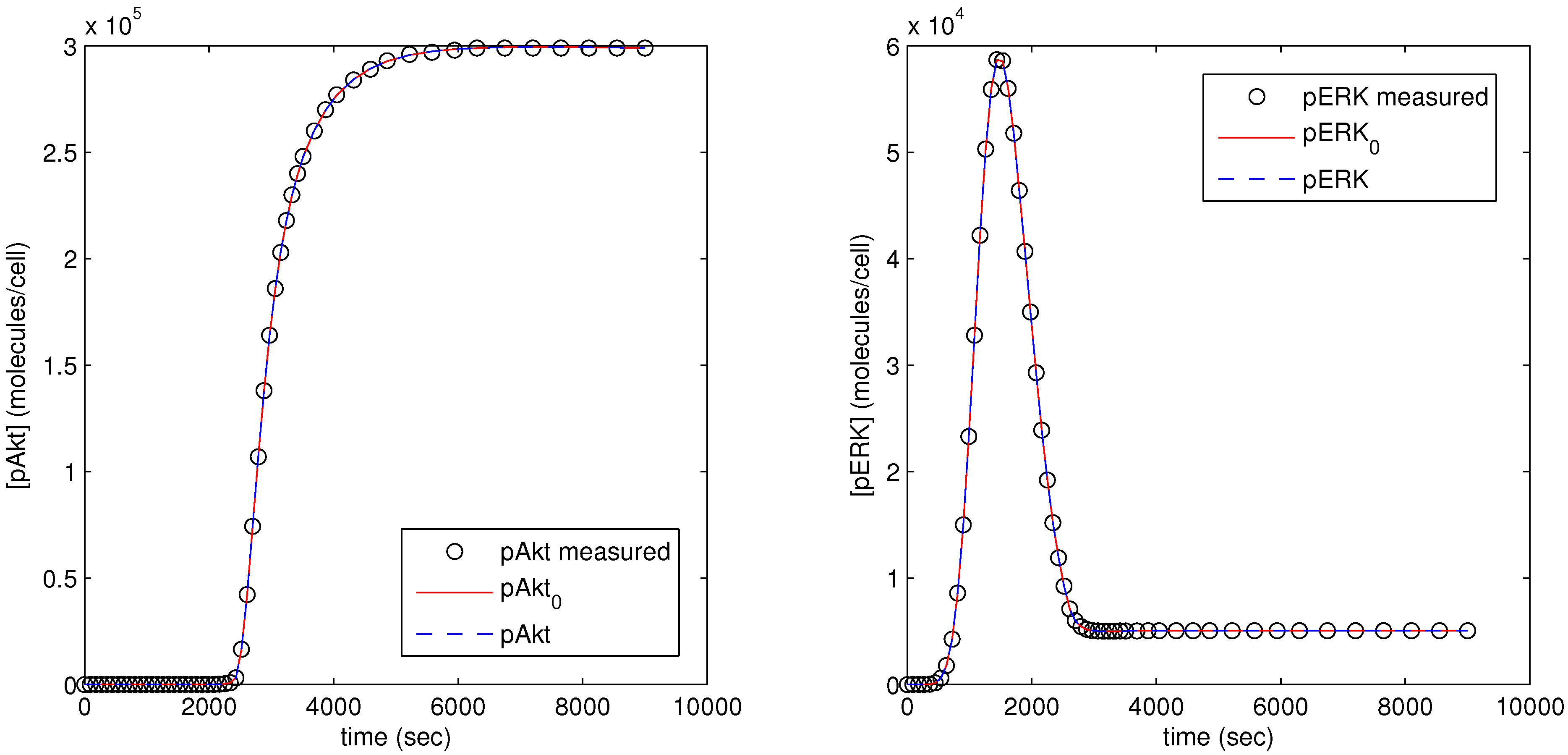
The parameter optimization fits the model parameters to data available for the pAkt and pERK state variables. In Figure 12, the dots (pAkt measured, pERK measured) represent the measured values of the state variable, the blue line (pAkt, pERK) shows the fit after the parameter optimization, and the red line (${\mathrm{pAkt}}_0$, ${\mathrm{pERK}}_0$) indicates the model fit after the initial cold start solution.

The simultaneous parameter optimization showed a significant improvement to the previous capabilities of solvers utilized for the ErbB model. However, it is unlikely to converge to a solution if too many parameters are perturbed and optimized at once. With a simultaneous approach, several more model parameters are optimized in a group, given that the parameters are carefully selected in the methods above. While the actual parameter values are not always returned, the overall fit to data is retained, again emphasizing the point brought out by Gutenkunst et al. [50] that an overall fit is more essential than the actual model parameter values. The CPU times required for solution with different numbers of parameters optimized are shown in Table 1. The tests were performed on an Intel(R) Core(TM) i5-3210M CPU @2.50 GHz with 6.00 GB of RAM.

Figure 11. Lower block triangular form of ErbB model with original sparsity on the left and rearranged sparsity with successive blocks of variables and equations that are solved successively.

Figure 11. Lower block triangular form of ErbB model with original sparsity on the left and rearranged sparsity with successive blocks of variables and equations that are solved successively.

Figure 12. Results of parameter optimization with pAkt and pERK measurement as model objective.

Figure 12. Results of parameter optimization with pAkt and pERK measurement as model objective.

Table 1. CPU times for solution of ErbB model with hybrid and simultaneous methods.

Parameters	Hybrid	Simultaneous
1	33.2 s	30.6 s
3	50.4 s	45.4 s
5	41.5 s	67.8 s
10	75.3 s	failure

Table 1. CPU times for solution of ErbB model with hybrid and simultaneous methods.

Parameters	Hybrid	Simultaneous
1	33.2 s	30.6 s
3	50.4 s	45.4 s
5	41.5 s	67.8 s
10	75.3 s	failure

Optimizing for ten parameters with the hybrid approach resulted initially in a failure to converge, but it is observed that a successful solution is found by skipping co-linear parameters in the sensitivity ranking. This failure is due to original combination of parameters that have the same scaled effect on the predictions with a combination that should be optimized as a single parameter instead of as separate parameters.

Post-Processing Analysis and Parameter Sensitivity

The order in which parameters are estimated is determined by the parameter sensitivity with respect to model objective functions. The sensitivity analysis shows that the measured variables have no sensitivity to some parameters. These parameters, as well as zero-valued parameters, are kept at original levels without perturbation given that the perturbation of any one of these parameters would introduce additional pathways in the kinetic mechanism. Given these constraints, the sensitivity analysis shows that only 140 of the 225 rate constants in the ErbB model can be estimated. The remaining parameters are ordered from the most sensitive to least sensitive, and the most sensitive parameter is optimized first. In subsequent optimizations, additional parameters are perturbed and optimized in conjunction with the parameters from previous optimizations. That is, in the first run, the most sensitive parameter is perturbed and optimized, in the next run the two most sensitive parameters are perturbed and optimized simultaneously, and so forth.

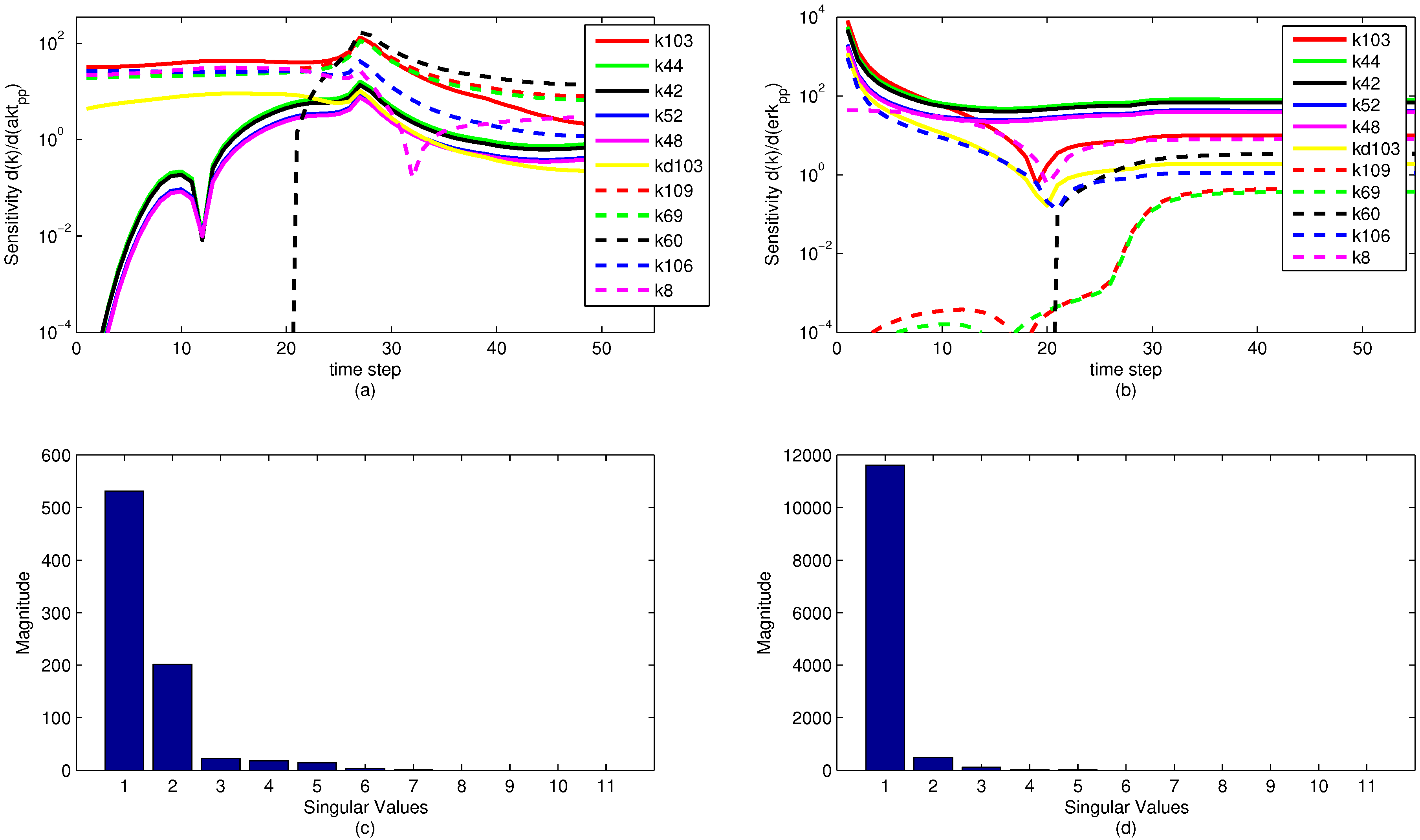
A sensitivity analysis is performed on the model parameters with respect to the model objective functions. The sensitivity is in reference to the two measured state variables to which the model is fit, namely pERK and pAkt. The results of the sensitivity analysis are shown below in Figure 13. Note that the model parameters have different sensitivities at different time points. It is significant to note that while a model parameter may not have a large effect on the objective over the dynamic time horizon (ranging from time step 1 to 35), the parameter can have a large effect on the steady state portion of the model. This reveals an important insight for the sensitivity ranking. If only the end sensitivity with respect to the objective function is considered for a model parameter, it may give a misleading result. A parameter that has low sensitivity at the end of the time horizon may in fact be a critical parameter early on. This principle is seen in the parameter $k_{60}$, which has zero sensitivity at the start of the time horizon but by the end has a significant sensitivity. In this particular case, the sensitivities of each parameter with respect to both pAkt and pERK are averaged over the entire time horizon and ranked accordingly.

The sensitivity plots may have some discontinuities in the first derivative (shown as sharp peaks or valleys) for two reasons. First is a natural discontinuity that occurs due to the indicator variables used in the model. At time step 21 ($t=1800s$), some model parameters are turned off and others are turned on with a piecewise function for the model that changes at time step 21. This results in a change in model dynamics, as seen in Figure 13a,b. The other discontinuities come from an algebraic manipulation of the log scaling. Because some of the sensitivities are negative-valued, they do not display on a logarithmic plot. The sensitivity plot shows the log value of absolute value of the sensitivity with respect to the given state variables. Because some of the parameter sensitivities change suddenly from positive to negative, there is a natural discontinuity in the first derivative.

Some interesting phenomena are apparent from the sensitivity graphs. Parameters that are scaled duplicates are co-linear or dependent parameters and are therefore impractical to optimize at the same time. For example, the two parameters $k_{44}$ and $k_{42}$ exhibit this paired relationship, and at all time steps the two sensitivities are proportional. In this case, either a linear combination of the parameters is estimated or one parameter is removed by the sensitivity selection process. It is possible, however, that parameters that appear to be pairs have different nonlinear sensitivities and the same graphical behavior is not observed as the parameters are adjusted throughout the parameter estimation. This behavior is not shown in the sample parameters in Figure 13 nor is it pursued in this study, although it could potentially reveal some insight about parameter optimization.

Figure 13. Parameter sensitivity over the time horizon (subplots a and b) and singular value magnitudes for principal parameter search directions (subplots c and d). The relative levels of the singular values show that some parameters have a strong effect on the predictions while others have a minimal effect or are co-linear and do not need to be estimated.

Figure 13. Parameter sensitivity over the time horizon (subplots a and b) and singular value magnitudes for principal parameter search directions (subplots c and d). The relative levels of the singular values show that some parameters have a strong effect on the predictions while others have a minimal effect or are co-linear and do not need to be estimated.

The results of a singular value decomposition (SVD) [88] performed in MATLAB are shown in Figure 13c,d. This analysis is an essential step in understanding the number of parameters to be estimated in the model. For the eleven most sensitive parameters shown, Figure 13 shows that when evaluating the sensitivities with respect to the pERK predicted value, only three of the parameters have a significant influence on the objective, while about six of the parameters have an effect on the pAkt predicted value. The SVD analysis is also informative in minimizing the number of parameters needed for estimation by relating parameters that can be expressed as combinations of sets of other parameters. The methods behind the recombination of parameters are beyond the scope of this paper, but there is a possibility for reformulating models to minimize the model size and number of parameters to be optimized.

4. Discussion

The non-identifiability of many biological models leads to difficulties in parameter estimation, and several methods are shown to improve model convergence, including log scaling of the model parameters, sensitivity ranking, choosing correct perturbations, and structural decomposition. Further, a single strategy among these elements is insufficient to lead to a successful solution, but the combination of all of these elements improved the solution time. In the successive initialization and parameter estimation, each of these methods is implemented one at a time, improving intermediate solutions until the original problem is solved.

The simultaneous optimization of multiple parameters is a particular challenge in the ErbB case study. Only after the SVD analysis is the difficultly attributed to the actual model structure rather than the solver. The SVD analysis shows that it is impractical to optimize more than a small subset of independent parameters to achieve a proper fit. Perturbing and optimizing any other parameters has a negligible effect on the overall fit because of the low sensitivities magnitude. This study shows that the solver algorithms used for parameter optimization in dynamic biological models are effective in reducing the computational time (144,000 CPU min [20] for simulated annealing, a sequential method, versus approximately 1 CPU min for either the hybrid or simultaneous method) for parameter estimation.

The parameter sensitivity analysis reveals that different measurements of objective functions result in different numbers of parameters that can be optimized. The ErbB case shows that an evaluation of the objective function by minimizing the pAkt value results in more distinct parameters with significant sensitivity. This can be used to estimate more parameters within a model. By increasing the diversity of the data to which the model is fit, different parameter sets can be estimated based on a similar sensitivity analysis. The challenge, of course, comes in the fact that obtaining additional data for parameter fitting is costly and sometimes impossible. A more sophisticated model may capture more dynamics, but may require more experimental measurements in order to uniquely identify parameters.

5. Conclusions and Future Direction

A contribution of this work is to demonstrate the ability of hybrid simultaneous and sequential solvers to optimize sets of parameters in models typical of systems biology. Furthermore, model reformation strategies are proposed to increase the likelihood of a successful solution. A sensitivity analysis over the entire time horizon provides particularly sharp insights into the behavior of the model. This sensitivity analysis provides a contribution to the knowledge of the ErbB model and reveals insights that may allow optimization of additional model parameters. A conversion tool from SBML to APMonitor is created to facilitate the solution of systems biology models with the given methods. Finally, a benchmark test on these solvers is conducted to show the most effective solvers and combinations of solvers for solution of systems biology models.

The sensitivity analysis proved to be particularly insightful revealing parameters that are co-linear or else produce little change in the model predictions for the two measured values. Singular value decomposition (SVD) identifies parameters that have the largest influence on the model fit as well as parameters suitable to be combined into pseudo-parameters that are linear combinations of the original parameter space.

Two case studies are considered to test the applicability of the proposed hybrid method in comparison with a simultaneous solution. The HIV model provides a proof of concept and demonstrates that these methods can successfully simulate literature values of the model with the different approaches. The ErbB model reveals several important aspects of model identifiability and highlights some of the difficulties typical of biological models. Initialization methods are employed, including log scaling, sensitivity ranking, choice of solver, and cost and identifiability.

The original basis of the testing on biological models is to demonstrate the ability of the solvers to handle the unique challenges in large-scale biological models. The ErbB model highlights some other significant aspects of the optimization techniques and demonstrates that the sensitivity analysis predicts some of the issues with the model formulation. Future work can extend these methods to other large-scale biological models and remove the limitation of simplified models due to computational concerns.

While only the APOPT solver is used for the analysis of the two case studies, further work could expand to investigate the effectiveness of different solvers and combinations of solvers. While this idea is touched upon in this study, it has not been fully developed and could lead to further improvements in the optimization of systems biology models. Other optimization techniques such as simulated annealing or a genetic algorithm can be used to further investigate model parameter estimation in biological models.