Next Article in Journal
Experimental Characterisation of Fluid Mechanics in a Spinner Flask Bioreactor
Next Article in Special Issue
Song, H.-S., et al. Mathematical Modeling of Microbial Community Dynamics: A Methodological Review. Processes 2014, 2, 711–752
Previous Article in Journal
Energy Considerations for Plasma-Assisted N-Fixation Reactions
 
 
Correction published on 14 September 2015, see Processes 2015, 3(3), 699-700.
Review

Mathematical Modeling of Microbial Community Dynamics: A Methodological Review

Biological Sciences Division, Pacific Northwest National Laboratory, Richland, WA 99352, USA
*
Author to whom correspondence should be addressed.
Processes 2014, 2(4), 711-752; https://doi.org/10.3390/pr2040711
Submission received: 11 August 2014 / Revised: 17 September 2014 / Accepted: 29 September 2014 / Published: 17 October 2014

Abstract

:
Microorganisms in nature form diverse communities that dynamically change in structure and function in response to environmental variations. As a complex adaptive system, microbial communities show higher-order properties that are not present in individual microbes, but arise from their interactions. Predictive mathematical models not only help to understand the underlying principles of the dynamics and emergent properties of natural and synthetic microbial communities, but also provide key knowledge required for engineering them. In this article, we provide an overview of mathematical tools that include not only current mainstream approaches, but also less traditional approaches that, in our opinion, can be potentially useful. We discuss a broad range of methods ranging from low-resolution supra-organismal to high-resolution individual-based modeling. Particularly, we highlight the integrative approaches that synergistically combine disparate methods. In conclusion, we provide our outlook for the key aspects that should be further developed to move microbial community modeling towards greater predictive power.

Graphical Abstract

1. Introduction

Microbes are virtually ubiquitous on earth; they can be found in almost all aquatic and terrestrial environments, and are associated with all species of plants and animals. By some estimates, the total microbial biomass in the biosphere may nearly equal that of higher plants [1]. Microorganisms have a profound impact upon natural and engineered ecosystems, serving as key catalysis of biogeochemical reactions which are needed to sustain a robust and diverse biosphere. At a time in human history when the Earth appears to undergo a rapid change in climate, understanding the control mechanisms whereby microbial communities determine ecosystem function is particularly relevant.
The role of microorganisms is significant also in human health and disease. With approximately 16 million humans dying from infectious diseases each year [2], there is an increasing appreciation for the role of the “human microbiome” in conditions ranging from metabolic diseases [3], aging [4], and central nervous system disorders [5]. Microorganisms also play key role in a variety of industrial processes, including food production, mining, pulp and paper processing, and waste water treatment, as well as energy, biomaterials, and drug manufacturing [6].
Nonetheless, it is less appreciated that, in virtually in all of these settings, microbes do not function in isolation but rather as members of communities. Microbial communities are defined as multi-species assemblages, in which organisms live together in a contiguous environment and interact with each other [7]. Their complexity may range from dozens of “species” in extreme environments [8], to many hundreds (for example, on specific habitats on humans [9]) to tens of thousands per gram of soil [10]. Such complexity constitutes a major challenge for studying the relationships between the physiological behavior of individual species and ensuing interactions, which give rise to higher-order properties such as stability, productivity, and resiliency.
In the analysis of microbial communities, important challenges include quantification of fluxes through pathways for nutrient resource and energy, identification of interactions of populations with each other and their environment, and inference of system’s higher-order properties. For example, metabolic diversity and functional redundancy are thought to increase robustness to environmental perturbations, as extreme conditions are less likely to kill all species performing a particular ecological function. However, there is less understanding of the mechanisms that maintain diversity in microbial communities [11], which ostensibly are a key to the functional stability of the inhabited ecosystem.
This perspective suggests that microbial communities can be considered “complex adaptive systems”. That is, they are comprised of a network of spatially distributed agents that respond concurrently to the actions of others. The coherent behavior of the system then can arise from a variety of interactions between agents as well as with their local environment. Microbial populations and communities often exhibit much larger changes in biomass, composition, and activity than do plant and animal populations. These complex, nonequilibrium dynamics are driven by the temporal frequency of changes in both important environmental factors, the physiological responses of individual cells, and also the interactions among cells. The characteristic time for these processes can vary over 9 orders of magnitude from an enzymatic reaction to seasonal community succession (Figure 1). Systems with this level of complexity require simulation models to codify our current level of understanding of system dynamics. In the literature, there are a variety of mathematical approaches. In general, the level of complexity and details of models would be determined based on the goal of simulation and the time and length scales of target systems. Thus, the suitable choice of a framework requires the correct understanding of the strength and limitation in its application.
Figure 1. Characteristic time and length scales for various biological processes.
Processes 02 00711 g001
In this article, we review various mathematical approaches developed for simulating microbial community dynamics. While a number of published studies have offered insightful perspectives on this subject (e.g., [12,13,14,15,16,17,18]), the present review is unique in the following aspects. First, instead of being confined to specific applications, we cover a wide range of frameworks developed for modeling diverse systems such as biofilms, biogeochemical cycling (in soil or ocean), human microbiota, biotechnology processes, etc. Second, this review is focused on comparatively understanding methodologies. Thus, we discuss the structural characteristics of various frameworks including top-down methods, bottom-up formulations, and their integration. Third, beyond the frameworks most frequently used for microbial community modeling, our discussion extends to those that are less common but potentially useful; the latter include population balance models, thermodynamically-based models, and cybernetic modeling approaches. Finally, we provide a systematic understanding of various modeling frameworks by classifying them according to modeling units and the ability to describe heterogeneity. Thus, we organize this article as follows. After providing brief backgrounds (Section 2), we discuss different forms of modeling frameworks: Supra-organismal approaches (Section 3), population-based models (Section 4), formulations to account for spatial and population heterogeneity (Section 5), and advanced simulations based on model integration (Section 6).
Despite their usefulness, some mathematical methods could not be included in this review. To say a few, they include (i) tools for studying the processes and factors controlling microbial colonization and community assembly on a macro-scale (e.g., the approach by Stegen et al. [19]) and (ii) models for simulating cell-to-cell communication (such as quorum sensing) on a micro-scale (e.g., as described in [20]).

2. Background Information

Before embarking on a detailed discussion of individual approaches, we define modeling units for classifying models into different categories and symbolic notations to be used throughout this article.

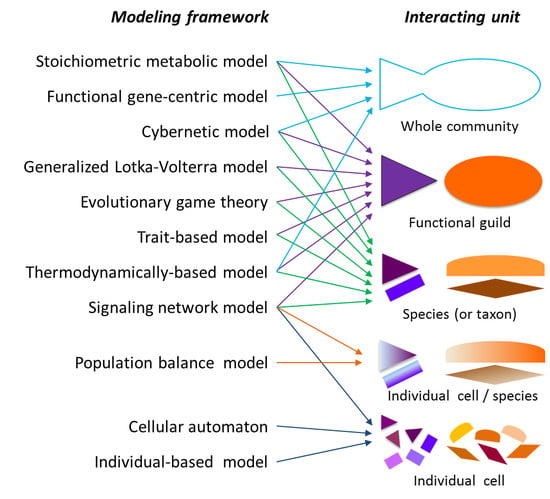
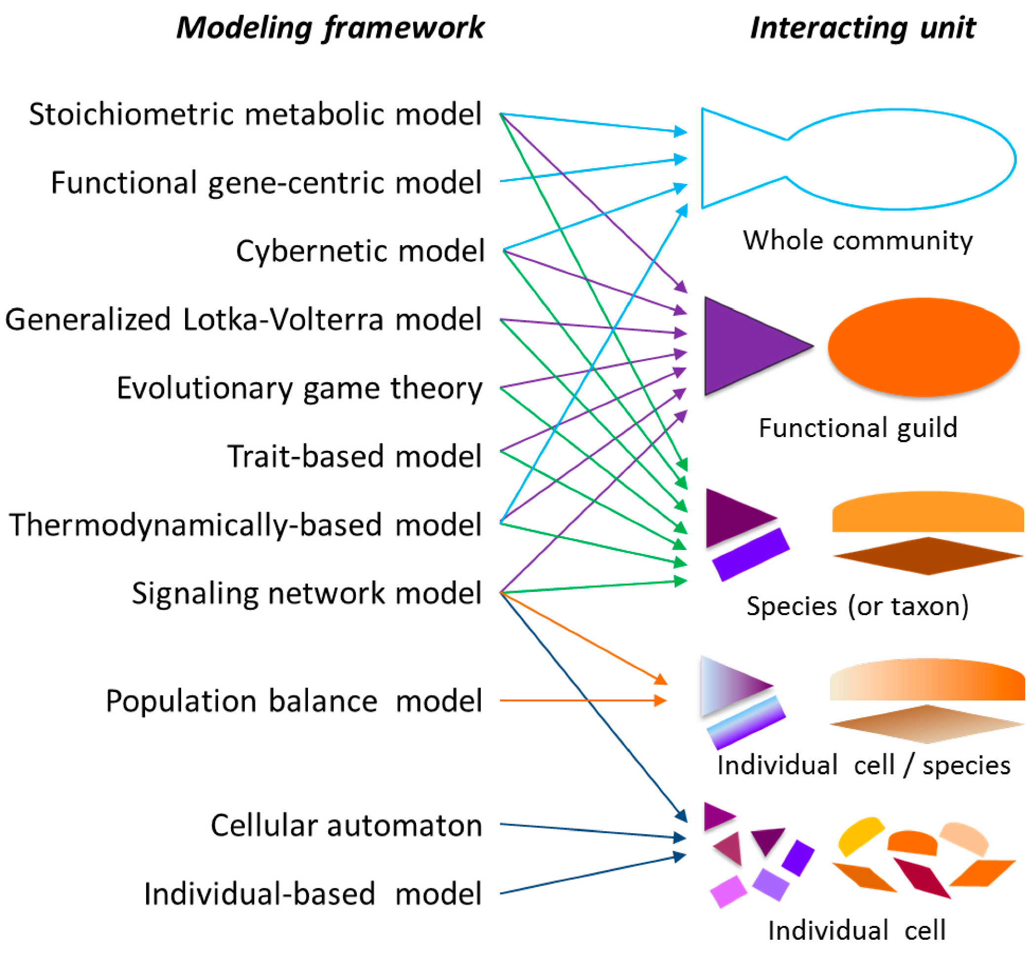
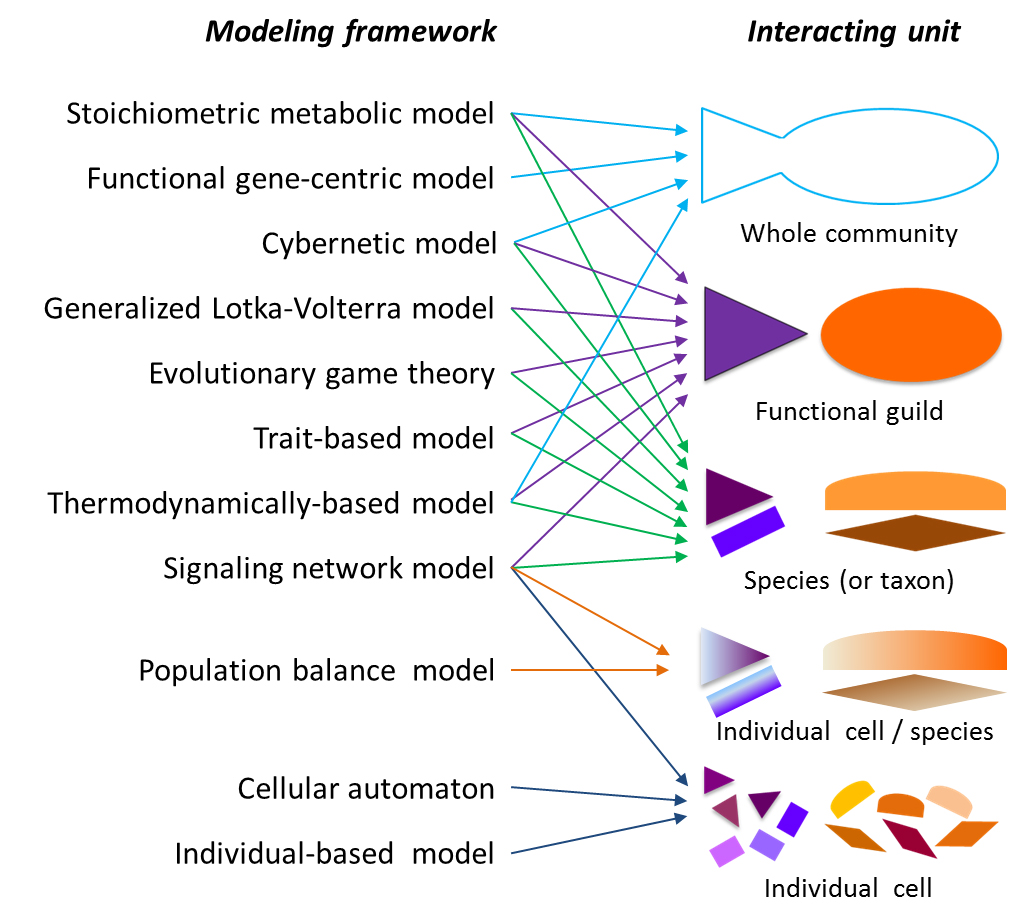
2.1. Modeling Units and Model Classification

Modeling units represent the basic entities that are modeled as interacting with each other within the microbial communities and their environment (or host). Predicted outcomes of interactions between the modeling units are community-level functions and properties. In this regard, we may call modeling units as “interacting units”. Depending on the choice of these units, the community dynamics can be simulated at different resolutions. Below, we address various modeling units commonly used in the literature: Individual cells, species (or taxa), functional guilds, or the community as a whole.
At a coarse level, some researchers have chosen the microbial community as a modeling unit, whereby a microbial community is treated as a supra-organism (or also called super-organism) performing various functions. From this angle, the microbial community can be viewed as a collection of genes and reactions, rather than a set of distinct species; consequently, models based on this concept describe the dynamics of microbial communities in terms of interactions between genes/reactions, rather than between species. The same abstraction has been used in comparative metagenome analyses that examine the entire set of genes of the community without identifying the gene’s species of origin [21].
More frequently, the dynamics of microbial communities have been simulated in terms of interactions between species (or taxa), whose functions can be distinct or redundant each other. Work in this area has been accelerated by the capacity to determine community composition and species abundance using advanced metagenomics and bioinformatics techniques. Many researchers take advantage of these species or taxa-level information for modeling. Alternatively, a group of species that possess functional similarities can be taken as the modeling unit. Metabolic functions of species are similar in each functional guild, but distinct from those of other groups. For example, in biogeochemical modeling based on this concept, functional guilds represent various metabolic groups associated with distinct electron donors and acceptors, e.g., catabolizers of polysaccharides, proteins, and monomeric organic C, and respiratory guilds of different types.
Emergent properties of microbial communities would be best studied by considering interactions at a single-cell level. Taking individual cells as the modeling units is justified considering that internal states and phenotypic traits of individual bacterial cells can be highly heterogeneous in populations, even in isogenic ones [22]. For example, a recent experimental study [23] showed that the internal state (i.e., the level of internally stored nutrients) of cells can vary significantly in a population.
In summary, supra-organismal approaches take the whole community as the modeling unit that interacts with environment. In population-based approaches, species (or taxa)/functional guilds are taken as interacting units. Variation in the population can be accounted for by using more rigorous frameworks such as population balance model (PBM) [24] and individual-based model (IbM) [25]. The most pronounced difference between them is that PBMs treat each population as a continuous phase, while IbM describes it as a collection of discrete particles. Figure 2 shows a broad classification of mathematical models based on the modeling (or interacting) units addressed above.
Figure 2. Classification of community models depending on interacting units. Individual shapes represent independent interacting units. Variance of state and functions across interacting units is represented by different colors. Color gradient in population balance model implies the heterogeneity in states and functions within the interacting unit. Representation of microbial communities using a fish shape is inspired by Scheffer et al. [26].
Processes 02 00711 g002

2.2. Mathematical Notations

For a systematic discussion, we define symbolic notations that are consistently used across different mathematical models. Notations unlisted below will be explained individually, wherever appropriate.
Vectors and matrices:
  • c = [c1, c2,…,cI]: The vector of concentration of J extracellular metabolites (such as substrates and produced metabolites) in environment
  • rk = [r1,k, r2,k,…,rJk,k]: The vector of Jk fluxes (or reaction rates) for species k
  • Sk: (k × Jk) Stoichiometric matrix of species k
  • x = [x1, x1,…,xK]: The vector of relative abundance or biomass concentration of K species
Indices:
  • I = [1,2, …,I]: Indices of I metabolites in environment
  • I΄k = [1,2, …,k] Indices of k intracellular metabolites for species k
  • Jk = [1,2, …,Jk] Indices of Jk fluxes for species k
  • K = [1,2, …,K]: Indices of K species
Scalars:
  • Yi,k: The yield of metabolite i for species k
  • Yx,k: The biomass yield of species k
  • µk: The growth rate of species k

3. Supra-Organismal Approaches

Supra-organismal approaches focus on the interactions of the whole community with the environment without considering cell boundaries. These models have been applied to many domains of life [27] including insect colonies and viruses, as well as microbial species, and are particularly applicable for the analysis of large-scale complex communities, such as those found in human, soil, and marine microbiomes, the number of whose member species is tremendous. An important advantage of taking supra-organismal approaches is that diverse modeling approaches developed for analyzing single organisms are readily applicable [28], which include stoichiometric [29,30] and dynamic modeling frameworks [31,32], as discussed below.

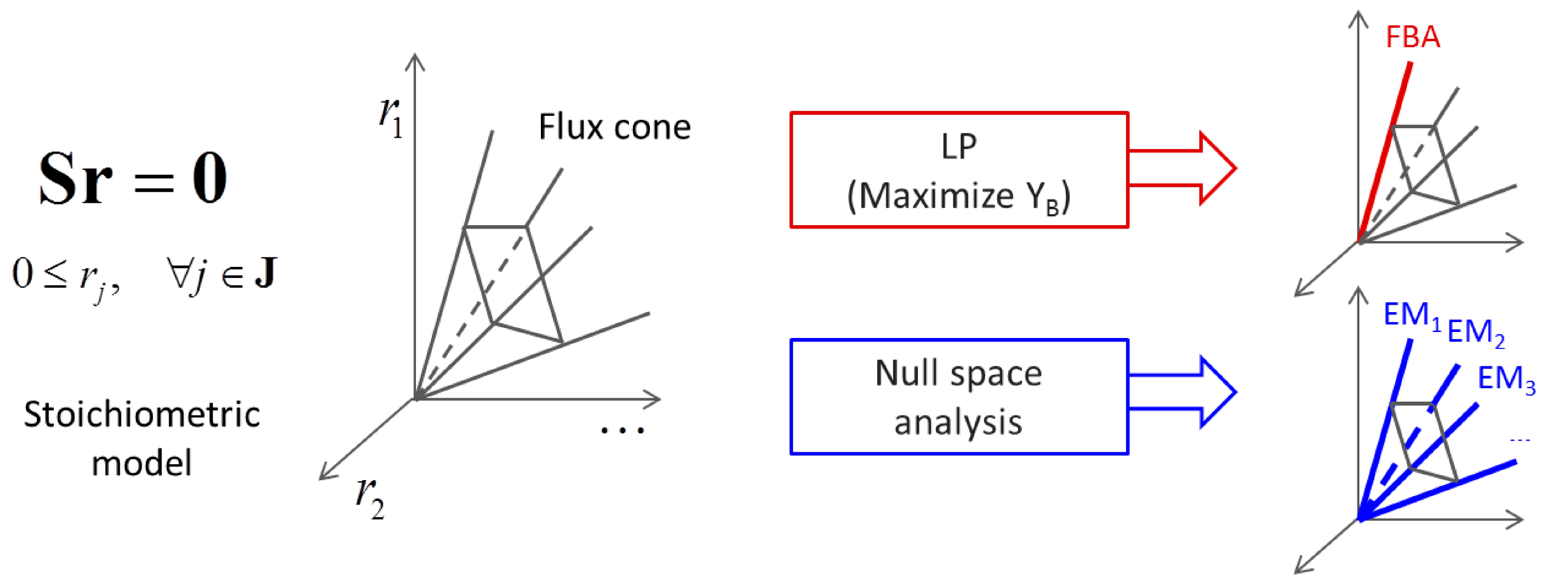
3.1. Stoichiometric Model-Based Analysis

A metabolic network contains a set of metabolites, their physical transport (into and out of an organism or a cell), and intracellular enzymatic biochemical conversions. The network can be represented as a graph that shows the connection of all metabolites (nodes) through reactions (links or arrows) or as a list of mass balance equations around metabolites (see Figure 3 as a tutorial example).
Figure 3. Graphical and mathematical representations of metabolic reactions occurring in a cell.
Processes 02 00711 g003
At steady state, the mass balances of intracellular metabolites (i.e., m1 and m2 in Figure 3) are given as a set of algebraic equation as follows (Figure 3):
Sr = 0
Where S is the ( × J) stoichiometric coefficient matrix and r is the column vector of J fluxes. Without loss of generality, we assume that Processes 02 00711 i001 
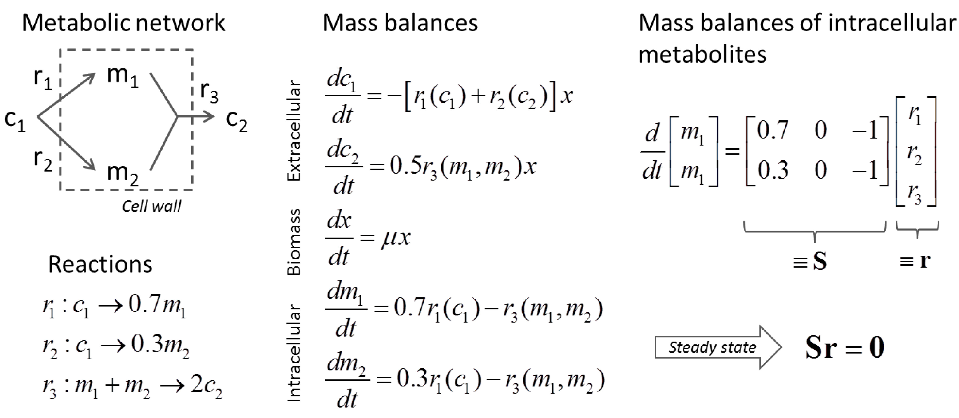
(by splitting reversible reactions into irreversible pairs). Together, the mass balances given in Equation (1) along with appropriate flux bounds are called stoichiometric models. Metabolic network models are often represented in a standard format called the Systems Biology Markup Language (SBML).
As < J in general, the solution vectors r satisfying Equation (1) form a convex polyhedral cone in a flux space (thus, called flux cone). Using stoichiometric model-based methods such as flux balance analysis (FBA) [29] and elementary mode (EM) analysis [30], it is possible to estimate a specific metabolic state of an organism through the identification of relevant metabolic pathways presumably active in a given steady state. Figure 4 shows how FBA and EM analysis perform differently. FBA assumes metabolism in a single microbe to be represented by an optimal pathway that maximizes the production of biomass (or any other metabolites including ATP). FBA obtains an optimal pathway by solving a linear programming (LP) problem subject to Equation (1) and inequality flux bounds. On the other hand, EM analysis identifies edge vectors (i.e., EMs) of the flux cone because convex combinations of all edge vectors can represent any feasible solutions within or on the cone. The full set of EMs is simultaneously computed using nullspace-based methods (e.g., [33]), but it is also possible to sequentially enumerate them using mixed integer linear programming (MILP) [34], a standard method for solving optimization problems in which some of the variables are constrained to be integers. Recent advances in numerical implementations [35,36] led to the computation of up to millions of EMs. A minimal set of EMs that represents a specific metabolic state can systematically be chosen using the methods reported in [37,38]. Nonhomogeneous constraints can be accounted for not only in FBA calculations, but also in EM analysis [39].
Figure 4. A schematic illustrating the concept of flux balance analysis (FBA) and elementary mode (EM) analysis.
Processes 02 00711 g004
Stoichiometric modeling approaches addressed above can be applied for the analysis of a microbial community based on the supra-organismal concept if a metabolic network is reconstructed for the whole community. A community-level metabolic network can be reconstructed as described by Greenblum et al. [40] in their in silico study of the human gut microbiome. Using the Kyoto Encyclopedia of Genes and Genomes (KEGG) database, metagenomic sequence reads were annotated to identify enzymes, the entire set of which found in any sample was then used to construct community-level metabolic networks for different conditions. While they focused on topological analysis as the resulting networks were noisy and inaccurate, community-level networks obtained as such are readily amenable to stoichiometric model-based analyses such as FBA or EM analysis.
Taffs et al. [41] provided an example of analyzing a community-level network based on EM analysis. The community considered therein contains three functional guilds, including unicellular cyanobacteria related to Synechococcus spp., filamentous anoxygenic phototrophs related to Chloroflexus and Roseiflexus spp., and sulfate-reducing bacteria. As individual networks for guilds were previously available, the community-level network was generated by superimposing them. This method (named as a pooled approach) formulating a set of functional guilds as a single network was compared with two other (i.e., compartmentalized and nested) approaches that consider individual networks separately. While the latter two approaches allow more detailed analysis on a microbial community by providing information on inter-guild interactions, the pooled approach is also useful for initial and exploratory analyses of complex or poorly understood communities as addressed by the authors.

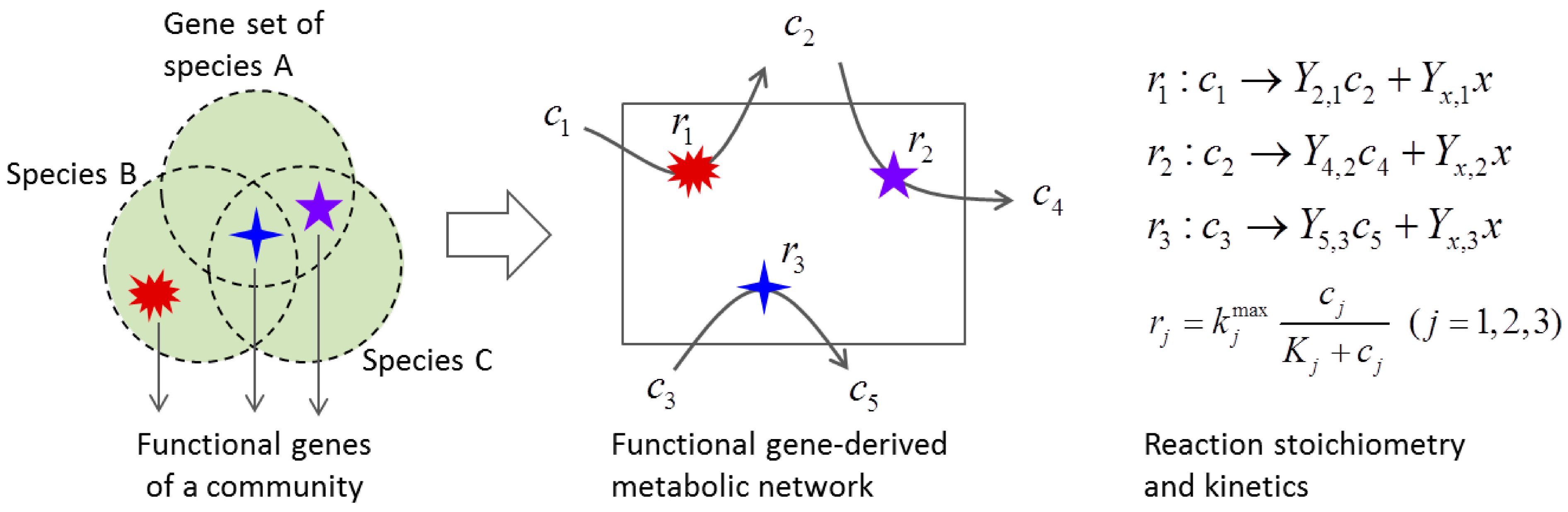
3.2. Metabolic Function-Based Dynamic Modeling

Stoichiometric analysis of metabolic networks helps to estimate the flux distribution within the community in a given environment. Simulation of the dynamic response of the community to environmental variations requires the use of modeling frameworks that dynamically adjust to the environment. For example, one would develop an adaptive model of a supra-organism based on primary metabolic functions performed by the community without knowing who provide those capabilities. A metabolic network of the community can be constructed with a focus on those primary metabolic functions catalyzed by a set of functional genes of interest (Figure 5).
Figure 5. Function-based dynamic modeling.
Processes 02 00711 g005
For the toy system considered in Figure 5, the dynamics of the community as a supra-organism can then be modeled as follows:
Processes 02 00711 i002
Processes 02 00711 i003
Where Yx,j and Yi,j denote the yields of biomass and extracellular metabolite ci through rj By focusing on a small number of key metabolic functions only, this approach reduces the difficulty of model identification generally arising when one considers a detailed structure of a metabolic network.
Along this line, Reed et al. [42] recently presented a gene-centric approach where they accounted for the dependence of reactions rj΄s on the level of functional genes, including the dynamic response of the function of each respective gene. That is, in the above above example,
Processes 02 00711 i004
Processes 02 00711 i005
Where ej represents the abundance of functional gene that catalyzes rj and λ denotes the mortality rate constant of a gene. In the case study of nitrogen cycling in the Arabian Sea, they developed a model based on eight functional genes associated with various metabolic functions such as aerobic respiration, nitrate reduction, nitrite reduction, dissimilatory nitrite reduction to ammonium, sulfate reduction, sulfide oxidation (coupled to nitrate reduction), aerobic sulfide oxidation, aerobic ammonia oxidation, anaerobic ammonium oxidation, and aerobic nitrite oxidation. Biomass yields were estimated from thermodynamic energy information, while stoichiometric coefficients of other metabolites were determined from elemental and electron balances.
It is challenging to apply the functional gene-centric approach to complex ecological systems containing diverse sets of electron donors and acceptors that represent alternative choices for exploitation by microbial communities. Their competitive relationship is often shown as a sequential consumption pattern. In many cases, including Reed et al., those patterns are simulated by designing the kinetics of rj’s as complex forms and/or additionally considering inhibition terms, but the incorporation of cellular regulatory actions would facilitate model development in a more systematic way. In this regard, while not applied yet, the cybernetic approach developed by Ramkrishna and coworkers [43] is well suited for simulating the community dynamics based on functional gene-centric approach. The cybernetic approach hypothesizes that cellular metabolism is optimally regulated to achieve a certain objective function that is related to actual rates rather than yields. Based on optimal control theory, the cybernetic approach then provides accurate predictions of cellular responses to environmental and genetic perturbations, without relying on mechanistic details of regulation (see [44,45,46,47,48,49] for examples of cybernetic modeling).
The successful application of the gene-centric approach addressed above requires known associations between functional genes and reactions. This can be a limitation because some of potentially important functions may be missed due to metagenomic coverage. Nevertheless, the dynamic simulation of microbial communities based on a supra-organismal concept is an attractive alternative when it becomes difficult to perform the full dynamics analysis at an individual species level.

4. Population-Based Models

Most commonly, the microbial community dynamics have been simulated at the level of individual populations of species or guilds. In these population-based modeling approaches, the internal states and phenotypic functions are assumed to be homogeneous across cells within each population. One of the main issues therein is how to account for interspecies (inter-guild) interactions in a direct or indirect (i.e., through environment) way for the prediction of community structure and functions. This section presents (i) static methods for inferring interspecies interactions and (ii) approaches for predicting community structure in a given condition and its dynamic change in response to perturbations. For the sake of simplicity, we confine our discussion to well-mixed environments. The issue of spatial heterogeneity is handled in a follow-up section.

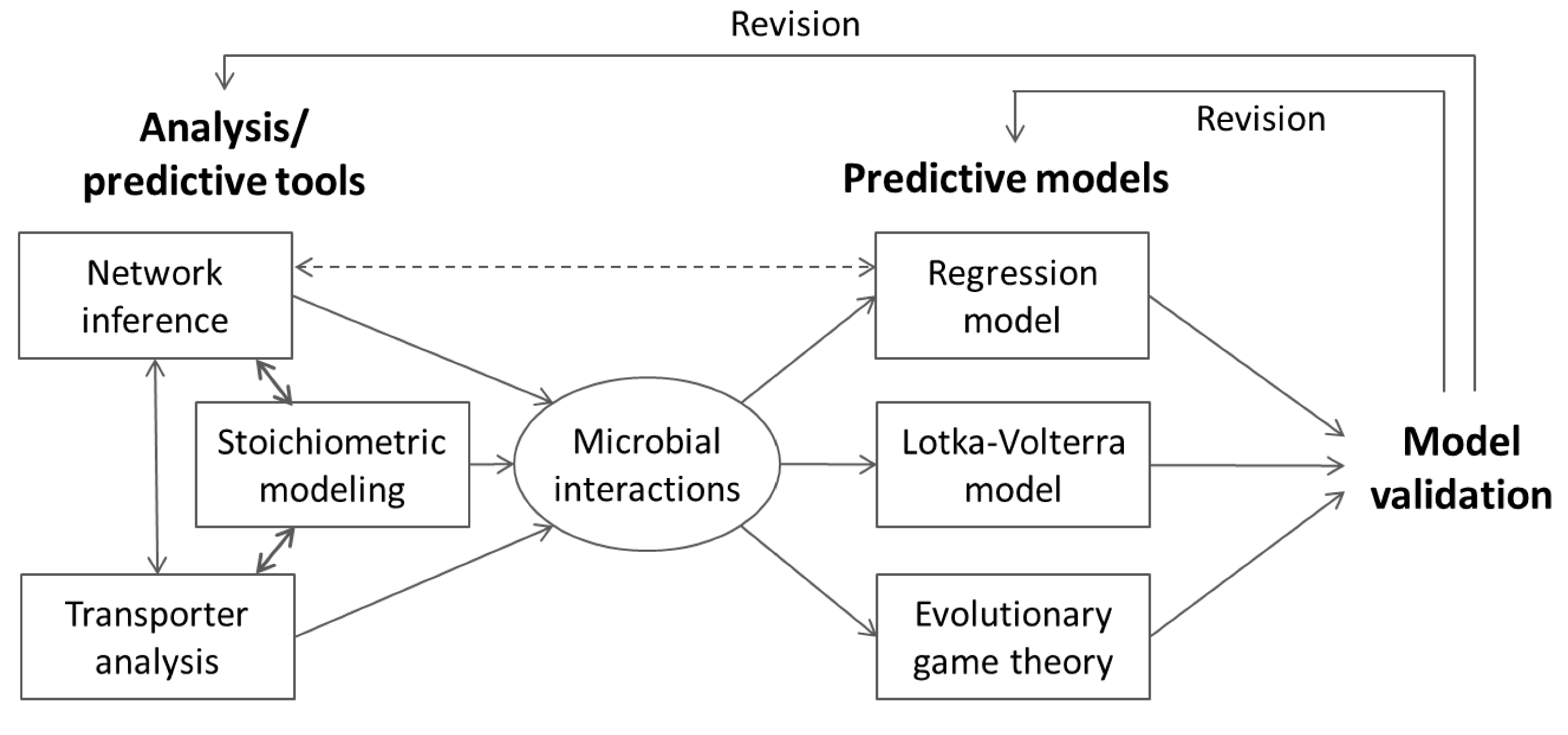
4.1. Inference of Microbial Interactions

In a community, microbes may exert a positive, negative, or neutral impact on each other. The positive (negative) impact of the species A on the species B implies that B grows better (worse) in the presence of A. The relationships between species can be bidirectional, if the impact is mutually positive (mutualism if obligatory, or synergism if nonobligatory), mutually negative (competition), or positive on one side but negative on the other (antagonism); unidirectional, if the impact on one of the two is neutral, regardless of whether the impact on the other is positive (commensalism) or negative (amensalism); non-directional, if the impact on each other is negligible or insignificant (neutralism) (Table 1) [50]. Neutralism is rarely found in natural microbial communities [51].
Table 1. Forms of microbial interactions: The positive, negative, and neutral impact of one species on another is represented by ⊕, ⊖, and ⊙, respectively.
RelationExamples
BidirectionalMutualism or synergism⊕⊕Biofilm formation to confer antibiotic resistance to the community members [52,53]
Syntropy (or cross-feeding): Hydrogen transfer between sulfate reducers and methanogens [54]
Competition⊖⊖Species with similar niches: Paramecium aurelia and Paramecium caudatum [55]
Antagonism⊕⊖Predation: Ciliates feeding on bacteria [50]
Parasitism: Bacteria and bacteriophages [50]
UnidirectionalCommensalism⊕⊙Acetobacter oxydans oxidizing mannitol to produce fructose, which is used by other species such as Saccharomyces carlsbergensis that can metabolize fructose, but cannot mannitol (http://www.eoearth.org/view/article/171918/)
Mycobacterium vaccae metabolizing cyclohexane to cyclohexanol, which is subsequently used by Pseudomonas species (http://www.eoearth.org/view/article/171918/)
Amensalism⊖⊙Lactobacilli producing acids that lower the pH of the surrounding environment [50]
The bread mold Penicillium secreting penicillin that kills bacteria [56]
Non-directionalNeutralism⊙⊙Growth of yogurt starter strains of Streptococcus and Lactobacillus in a chemostat [51]: The populations of these strains do not change much regardless of whether cultured separately or together
The nonrandom co-occurrence patterns of species observed in ecosystems may be interpreted that the community structure is shaped primarily by microbial interactions [57]. Basic microbial relationships can be studied by comparing the growth rates (or biomass concentrations) from individual-growth and co-growth environments, respectively. Experimental identification is often ineffective, however, due to the difficulty in isolating individual organisms for axenic growth experiments. Alternatively, we may use theoretical tools such as network inference methods or metabolic network analyses.

4.1.1. Network Inference

Advanced metagenomics and bioinformatics techniques allow for the identification of member species in the community and estimates of their relative abundances and functional capabilities [58]. “Shotgun” methods survey genomic content of a microbial community directly from the natural environment, without having to isolate individual species for lab cultivation. Sequence data can be segregated into bins representing distinct Operational Taxonomic Units (OTU), which may mean an individual organism or species, or a group that shares a certain set of observed characters. Two classes of binning processes include similarity-based (or align-based) and composition-based strategies [59]. Similarity-based binning searches for sequence similarities between samples and reference genomes in existing public databases. Composition-based methods cluster metagenomic sequences into different bins using intrinsic, organism-specific characters of the DNA sequence, such as GC content, dinucleotide frequencies, and codon usage bias. Bins can be analyzed to provide information about community composition and member abundances. In some case, near-complete genomic information can be recovered for some member populations.
Microbial relationships can be inferred from species abundance data. Based on the traditional perceptions, we may refer to the relationship of a pair of organisms as competitive (or negative) if their abundances across samples are anti-correlated despite they share environmental niches; as cooperative (or positive) if they show similar abundance pattern. The network of microbial associations can be predicted in a systematic way using the techniques termed as network inference. Similarity-based methods infer pairwise relationships by analyzing the co-occurrence/exclusion patterns of two species based on similarity scores. More complex interactions between more than two species can be captured using other techniques such as regression-based and rule-based methods. Regression-based methods represent the abundance of a certain species as a function of the abundances of other species. Rule-based methods initially enumerate all logically possible rules for the coexistence/exclusion of species as supported by presence-absence data sets. Only significant rules are retained through the subsequent filtering processes. Faust and Raes [50] provides an excellent review on this subject.
The identified relationships between the member species can be represented as a (microbial association) network composed of nodes (or vertices) and links (or edges). Nodes and links represent species (or taxa) and their interactions, respectively. The relationships between species are often asymmetric, i.e., the presence of one species can impact on the population of another, but not vice versa. The direction and strength of microbial interaction can be represented by an arrow and its thickness, respectively. Environmental variables can also be incorporated into the network by treating them as additional species. This expanded network reveals the relationship between species and environmental traits. For example, consistent co-occurrence between certain species and nutrients (e.g., nitrites and nitrates) indicates the involvement of specific microbes in biogeochemical cycles [60].
Like other robust networks (including World Wide Web, protein-protein interactions, cellular metabolic systems, and human social networks), microbial association networks are scale-free [50]. The scale-free network is characterized by a majority of species with only a few links (i.e., low-degree nodes) and a few hub species with many links (i.e., high-degree nodes). The degree distribution of a scale-free network follows a power law, a semi-log plot of which gives a straight line [61,62]. Scale-free networks are robust against random deletion of nodes, but this tolerance comes at the cost of extreme vulnerability to targeted removal of hubs [63]. This implies that a microbial community may malfunction when losing a hub species, but may perform normally after the loss of a functionally less-connected species. A group of species that are densely connected with each other may be interpreted as having overlapping niches [50]. An interesting and unresolved issue is the ecological role of hub and non-hub species.
Using the methods addressed above, microbial relationships can be systematically inferred from species abundance data. Microbial associations derived as such are condition-specific, meaning that information on microbial relationship obtained from one condition may not valid in another condition, as the structure and properties of microbial association networks can significantly be changed according to environmental conditions. Also, they do not provide biological reasons why certain species interact in a specific way while others do not. To gain a more mechanistic understanding, we need physiology-based tools such as the ones described in the following.

4.1.2. Stoichiometric Modeling of Multiple Species

Stoichiometric metabolic network-based analyses not only provide mechanistic insights on species interactions with each other and with their environment, but also estimate flux distributions within individual species and the community. Stoichiometric model-based analysis discussed in Section 3.1 can be used to model individual species/taxa in microbial communities. Figure 6 summarizes the process of developing a stoichiometric model for a multispecies system.
Figure 6. Procedures of developing a stoichiometric model for a simple microbial consortium. The metabolic networks and stoichiometric models for individual species are reconstructed based on species-level genes assigned through the binning process. The size of the resulting community stoichiometric model is increasing in proportion to the number of species.
Processes 02 00711 g006
In the pioneering work by Stoylar et al. [64], FBA was applied to analyze syntrophic relationship between sulfate-reducing bacteria (Desulfovibrio vulgaris) and methanogens (Methanococcus maripaludis). The community metabolic network combines individual species networks by treating them as internal compartments. They estimated interspecies metabolite flows, together with intracellular flux distributions in each organism by maximizing the weighted sum of species biomasses. Freilich et al. [65] used the method of Stoylar et al. [64] to predict metabolic interactions between two species for the 6903 pair-wise combinations of 118 genome-scale metabolic models of bacteria. They compared the biomass production rates between co-growth (CG) and sum of individual growth (SIG) to classify the interactions as competitive (if CG < SIG), cooperative (if CG > SIG), or neutral (if CG ≈ SIG). They also determined winners and losers for competitive pairs and givers and takers for cooperative pairs, along with the level of competition and cooperation.
Klitgord and Segre [66] extended the method by Stoylar et al. (by artificially introducing additional compartment that represents environment shared by different species) to explore interspecies metabolite exchanges for various pairwise combinations of seven bacterial species. Their algorithm not only recapitulated known cross-feeding interactions, but also discovered new sets of metabolites potentially exchanged. They also showed how to computationally identify culture media that lead to commensalism or mutualism for a given set of organisms. Wintermute and Silver [67] developed a computational framework based on the minimization of metabolic adjustment (MOMA) [68] to investigate the interactions in synthetic pairs of 46 Escherichia coli auxotrophs. As a result, they observed synergism in 17% of 1035 computationally identified pairs. Beyond microbial consortia, these joint stoichiometric modeling techniques have also been applied to simulate metabolic interactions between different organs in human [69] or between different cell types in an organ [70].
FBA-based formulation was applied to microbial communities under the name of community flux balance analysis (cFBA) [71]. Zomorrodi and Maranas [72] proposed a generalized computational platform for implementing cFBA. Their framework termed OptCom formulates a bi-level optimization problem where both community-level and individual cell-level objectives are maximized/minimized. Metabolic fluxes are estimated from the tradeoffs of those objective functions at individual species and whole community levels. Experimental data for the community (such as composition) and organisms (such as uptake rate), if available, can be incorporated to improve the quality of predictions. Zomorrodi et al. [73] recently developed a dynamic version of OptCom (called d-OptCom), which we discuss in Section 6.3.
The compartmentalized approach of Taffs et al. [41] used the same type of expanded networks (i.e., containing individual networks as compartments) for the EM analysis. The computational burden significantly increases, however, as the number of EMs undergoes combinatorial explosion with the network size. Thus, they alternatively suggested the nested approach, which first analyzes each of individual networks (which is computationally less demanding), and subsequently, examines the potential interactions between individual networks based on ecologically relevant pathways.
It will be difficult to extend metabolic network-based analysis to complex ecological systems containing lots of uncharacterized species, whose genetic and metabolic information are not well known. Analysis of an expanded community network constructed by combining genome-scale networks of individual species becomes also computationally demanding when the number of species is significantly large. This is true with the LP-based cFBA as the expanded number of reactions leads to huge memory requirement. While the current practice of these bottom-up analyses is therefore limited to simple consortia composed of a few species/guilds, their extension to more complex systems will be feasible in the future with the rapid progress of metaomics technologies and related experimental/computational methods.

4.2. Nonlinear Regression Models

In general, the dynamics of microbial communities are simulated using differential equation-based models. However, if one’s interest is to predict how microbes are assembled in a given environment and how the community composition changes across different conditions, non-differential equation-based approaches would also be useful. One approach along this line is to develop algebraic relationships between species abundances and environmental conditions using nonlinear regression techniques. Abundance of each species in the community can then be formulated either as a function of environmental variables only or in terms of both environmental factors and the abundance of other species.
Suppose that we have collected sets of species abundance data across different locations characterized with specific environmental traits. Alternatively, we may gather data on the temporal change of microbial community composition (at a fixed location) driven by seasonal climate variations. These data provide an opportunity to build a predictive model that combines species occurrence (or abundance) and environmental conditions. In the case that mechanistic information on microbial assemblage in response to external stimulations is unknown or difficult to collect, the relationship between species and environmental factors can be established through nonlinear algebraic equations. That is, for the community composed of K members, the abundance of the Kth member (xk) may then be represented as follows:
xk = fa,k(c,p), k = 1,…, K
where the vectors c and p denote environmental variables and parameters. Once the functional forms of fa,k’s and the set of parameters p are suitably identified, it becomes possible to predict species abundance in a new condition by providing environmental factors therein. Bioclimatic models often use this approach to predict the species abundance as a function of environmental conditions and its variation across a landscape, and are also called different names including ecological niche models and species distribution models [74].
Larsen et al. [75] proposed an extended form by incorporating biotic interactions, i.e.,
Processes 02 00711 i006
Here, the abundance of species k is described as being dependent on the abundances of other species, as well as environmental factors. They reported improved predictions of community structure in comparison to the cases excluding biotic interactions.
In general, sufficiently large datasets may be required to develop nonlinear regression models. Major challenges in developing them such as the one in Equation (7) include (i) the handling of a large number of potential interactions between species and environmental factors, which will be more problematic for complex communities; and (ii) the suitable formulation of nonlinear regression equations for each species. To focus on key interspecies reactions, the methods discussed in Section 4.1 (i.e., network inference and/or stoichiometric model analyses) would be critically useful. The design of appropriate functional forms can be facilitated by the use of specially designed software package such as Eureqa developed by Schmidt and Lipson [76]. Given sets of experimental data, Eureqa is able to identify the simplest form of a mathematical function that can best describe their correlation using symbolic regression method.

4.3. Thermodynamically-Based Models

Thermodynamically-based models potentially provide more mechanistic predictions on the change of community structure across conditions. Most researchers are familiar with the use of kinetic approaches, but thermodynamic modeling differs in the following several ways. Kinetics deals with absolute concentrations, while thermodynamics deals with relative concentrations. In kinetic models, time is modeled parametrically while in thermodynamic models, time can sometimes be modeled non-parametrically; that is, under certain assumptions thermodynamics can provide information on the rank order of reactions as they occur in time.
In most applications of thermodynamics to mixed microbial systems (including biorefineries, water systems, marine systems and biogeochemical remediation sites), the focus has been to predict or understand product formation without explicitly modeling all details of the chemical transformations that lie between initial environmental compounds and oxidized metabolites excreted by the environment. This is a task that thermodynamics is well suited for, since the thermodynamic functions of free energy and entropy are state variables whose values are independent of the path taken between initial reactants and final products. Biogeochemists, for example, typically use databases of geochemical reactions to model geochemical processes. Since biological oxidation and reduction can also occur, it makes sense to supplement databases of geochemical reactions with reactions mediated by microbial communities. Istok et al. [77] supplemented tables of geochemical reactions with thermodynamic-based growth equations of microbes and then predicted laboratory and field interventions for the bioreduction of uranium. Likewise, Larowe et al. [78] used thermodynamic modeling to evaluate and compare the driving forces responsible for microbial anaerobic methane oxidation across representative marine ecological sites and different consortia. The analysis showed that consortia with significant coupling to sulfate-reducing organisms have sufficient thermodynamic driving forces for methane oxidation.
The ability to predict product yields from models is also an important goal for biotechnology applications. Rodriguez et al. [79] used thermodynamically-based models to predict product yields from glucose fermentation in mixed cultures. While the nature of the modeling did not distinguish boundaries between individual species, the approach differed from those mentioned above in that intermediate reactions of metabolism were modeled and not just summary reactions. This approach is becoming popular for modeling situations in which only a metagenome is available.
The modeling of metabolism in detail for communities of organisms using thermodynamics is increasing and it is worthwhile to elaborate on the methods and assumptions used in these models. For an isolated reaction
Processes 02 00711 i007
the relationship between thermodynamics and flux has been inferred to be [80],
Processes 02 00711 i008
where G, R, and T denote Gibbs free energy, ideal gas constant, and temperature, and J+1 and J−1 are forward and reverse flux values of the reaction as defined below, i.e.,
Processes 02 00711 i009
Some authors appreciate that this stated relationship is an approximation based on reversibility and the validity of the use of Equation (9) depends on the context in which it is used. If one assigns flux values based on an experimentally or computationally determined free energy change,
Processes 02 00711 i010
then one is using the assumption of detailed balance. This relationship is only strictly valid at equilibrium for an isolated system. Even for an individual reaction with no change in free energy in a coupled reaction system at non-equilbrium, there is no physical requirement for the reaction to obey detailed balance. Likewise, if one assigns free energy values based on observed fluxes from a non-equilibrium system using Equation (9), then the calculated free energy values will not be correct.
Even though the relationship does not strictly hold for non-equilibrium systems, the assumption of detailed balance can be a useful tool if used carefully. A case in point, Noor et al. [81] have used Equation (11) as a framework for evaluating flux statistics at individual reactions. They pointed out that reactions near equilibrium act as kinetic bottlenecks in pathways that are overall far from equilibrium. This is a valid use of the assumption of detailed balance in that reactions at equilibrium in an otherwise nonequilibrium system are those for which the assumption is not severe.
Another widely used thermodynamic concept in metabolic modeling, whether single organisms [82] or communities of organisms [83], is entropy production. In flux-based modeling, entropy production is used as a constraint to reduce the solution space to a set of reactions that are more likely to be feasible ones. Using the net flux of a reaction, for example Jnet = J+1J−1 in the example above, the constraints are generally stated as,
Jnet∆G ≤ 0
The concept is that that entropy production for a spontaneous process must be positive, or analogously as stated above that the rate of free energy production must be nonpositive. Strictly speaking, while the concept that entropy production for a spontaneous process must be positive is correct, we know from statistical mechanics that it applies to the overall process and not necessarily to individual reactions. Fluctuations that decrease entropy production are well known and are an active area of research. Nevertheless, just as in the case of Equation (11), the assumption that Equation (12) applies to individual reactions can be a useful tool when used with care.
The concept of thermodynamics as the basis for natural selection has considerable theoretical and empirical justifications [84,85,86,87,88,89], and consequently modeling approaches have been developed that use maximum entropy production as either an optimization goal or simulation master equation. Zhu et al. have developed a flux-based approach that uses entropy production as the optimization goal [82]. While several flux-based applications include constraints based on Equations (9) to (12), this approach selects the thermodynamically most optimal solution as the most likely one.
Taking this concept a step further, new methods have been reported [90,91] that use statistical thermodynamics directly to solve a thermodynamic master equation similar to the kinetic master equation approach developed by Gillespie [92] and others. The kinetic master equation is a stochastic equation giving the probability of a state as a function of time. In the thermodynamic master equation, if the rates of the reactions are such that the system is thermodynamically optimal, then time can be modeled non-parametrically (e.g., rank ordering of time-dependent reactions). The master equation is based on an open system with the probabilities of individual reactions being determined by changes in the chemical potentials. The advantage of this approach over a flux-based approach that contains thermodynamic constraints is that approximations such as Equations (9) to (12) are not required and metabolite concentrations and energy requirements of pathways can be determined directly. The caveat, as mentioned above, is that if one does not have rate constants to work with, then some applications may need to assume that the rates of the reactions are such that the system is thermodynamically optimal.

4.4. Trait-Based Modeling

While species are considered the most natural units to describe the diversity and dynamics of microbial communities, taxonomic or phylogenetic distinction among species can become obscure as microorganisms often undergo rapid genetic changes through gene loss and gene acquisition via horizontal gene transfer. Thus, trait-based ecology characterizes organisms in terms of their functional properties by mapping organism-based information into a functional space [93]. The dynamics of microbial communities is then analyzed by focusing on the traits as the entities that mediate the microbial interactions with each other and the environment. Microbes can be classified by various traits such as morphological, behavioral, and biochemical similarities. The trait-based classification is thus taxon independent, i.e., it may lead to the combination of different species as the same group or the separation of the same species (if traits vary therein) into different groups. As modeling units, therefore, trait-based models often take a group of organisms (such as functional guilds) that share similar traits. The direct link of biological traits to environments makes trait-based models widely applicable to modeling behavior of a variety of living organisms in ecosystems [94].
Trait-based models have been used for the steady state and dynamic analyses of diverse ecosystems. For example, this methodology was used to predict the relative abundance of species for plant community assemblies in given environmental conditions. The review by Laughlin and Laughlin [95] is an excellent source regarding this subject. They compared two frameworks: The maximum entropy (Maxent) model (or Community Assembly by Trait Selection, CATS) [96,97] and the Traitspace model [98]. In both approaches, the community-level trait is represented as the sum of individual species trait. This generally leads to underdetermined systems with more unknowns (i.e., abundances) than equations (i.e., algebraic relations of traits between the community and individual species). The Maxent model estimates the relative abundance of species by maximizing the evenness (quantified as the entropy function) of their distribution. Thus, the Maxent solution has a tendency of broadening the distribution of species abundance. In contrast, the Traitspace that is based on Bayesian theory predicts an extremely low probability of abundances for functional groups that do not pass through so-called environmental filters. Thus, the resulting Traitspace solution contains a minimal number of species for a given condition. These approaches were used for the analysis of plant community assembly, but the concepts per se are interesting enough to be applicable to microbial communities as well.
Trait-based dynamic models, which consist of differential equations that represent the rates of change of nutrients, organic matter pools, populations of functional guilds, etc., have been applied to large-scale ecosystems, e.g., for studying ocean or subsurface biogeochemistry. In situations where phenotypic traits are distinct among functional guilds, the change of community composition in time can be predicted from the following population growth equations for K functional guilds, i.e.,
Processes 02 00711 i011
Where rk denotes the nutrient uptake rate of functional guild k and Yx,krk means its growth rate. Note that the reaction rate rk is a function of environmental variables, implying that Equation (13) describes species interactions as being made through the environment by competing for the nutrients or cooperating through metabolite exchanges. Balances of environmental variables are basically the same as Equation (3), i.e.,
Processes 02 00711 i012
Along this line, Jin and Roden [99] developed a biogeochemical model of batch sediment slurry to examine the influence of metabolic degradation of ethanol on the chemistry of anoxic subsurface environment. They grouped microorganisms into eight functional groups based on their metabolic capability of utilizing electron donors (ethanol and its intermediate products including acetate and H2) and acceptors (such as nitrate, ferric iron, sulfate, and bicarbonate). Thy then modeled twelve redox reactions that could contribute to ethanol degradation as being catalyzed by specific functional groups.
Bouskill et al. [100] introduced a microbial community trait-based modeling framework (MicroTrait) to study the nitrification (i.e., the process of oxidizing ammonia to nitrite and then nitrate) in the microbe-mediated nitrogen cycle. They simulated the nitrification process based on the eleven functional guilds: Seven Betaproteobacterial ammonia oxidizing bacteria (AOB), three nitrite-oxidizing bacteria (NOB), and one ammonia-oxidizing archaea (AOA). The model was then used to predict the diversity of nitrifying functional guilds and the rates of ammonia oxidation and nitrous oxide production across a range of environmental conditions.

4.5. Lotka-Volterra Model

The use of Lotka-Volterra (LV) type of models is an interesting alternative to simulate microbial population dynamics. The model was initially proposed by Lotka to analyze the predator-prey dynamics, while Volterra independently investigated the equations to explain oscillations in fish populations in the Adriatic. In addition to animal ecology, this model has been used to characterize the microbial population dynamics resulting from competitive and mutualistic interactions [101]. The generalized LV (gLV) equations are able to describe various possible relationships between arbitrary numbers of species. The gLV model represents the population growth dynamics of species k as follows:
Processes 02 00711 i013
Where akk΄ denotes the interaction strength between species k and . Unlike trait-based models discussed in the previous section, the gLV model directly considers the impact of the presence of other species on the growth of a certain species. The coefficients aij can be positive or negative or zero depending on the relationship between the two species. One the other hand, the gLV model above does not consider indirect species interactions through metabolite sharing or exchange.
Recently, the gLV equations were used to investigate microbial interactions in the human gut (e.g., [102,103]) and in a cheese microbial community [104]. In the study of the dynamics of intestinal microbiome structure, Stein et al. [103] extended the gLV equations by adding additional term describing the effect of environmental variations, i.e.,
Processes 02 00711 i014
where the last term on the right hand side of Equation (16) represents the impact of external variations on the growth of species k.

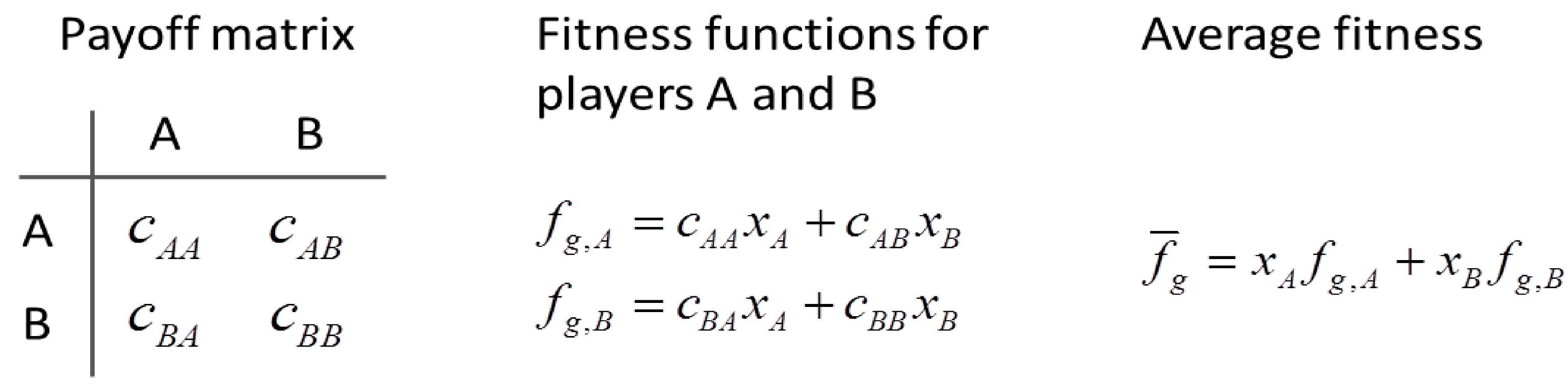
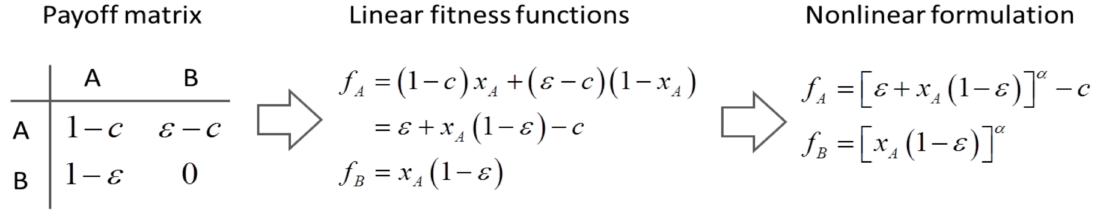
4.6. Evolutionary Game Theory

Classical game theory analyzes situations where the success of one’s choice (i.e., strategy) is influenced by the choices of other players. Fundamentally, this strategic game requires the players to make optimal choices by rationally analyzing all probable outcomes that would result from different combinations of strategies. A typical example for such strategic games is the prisoner’s dilemma. This concept of rationality has been used for the analysis of economic and social systems.
Without relying on the rationality of players, evolutionary game theory founded by the work of Maynard Smith and others [105] simulates the dynamic evolution of a certain strategy in a competing population, and evaluates how good it is. The success of a strategy is not only determined by its own quality, but also determined by the frequency (i.e., relative abundance) of other competing strategies in the population. This frequency-dependent selection concept implies that the fitness landscape is altered as the population structure and member abundance change with time [106].
Selection dynamics are typically represented using the following replicator equation, i.e.,
Processes 02 00711 i015
Where xk is the frequency or relative abundance of species k, fg,k is the fitness of species k, and fg is the average fitness represented as follows:
Processes 02 00711 i016
Equation (17) implies that the relative abundance of species k increases (decreases) if its fitness fk(x) is greater (less) than the average fitness of the population fg(x). Interestingly, the replicator equation is mathematically equivalent to the gLV equation: A replicator equation with n strategies can be transformed into a gLV equation with n − 1 species [105].
To provide an understanding of how evolutionary game-theoretic models are formulated, we consider a simple game between two strategies–say A and B. Figure 7 shows how fitness functions for players A and B, and the average fitness can be represented from the payoff matrix. The four entries in the payoff matrix are interpreted as follows: The player A gets payoff cAA when playing against A and cAB when playing against B; the player B gets payoff cBA when playing against A and cBB when playing against B.
Figure 7. A simple game between players A and B: In evolutionary game theory, payoff is equated with fitness.
Processes 02 00711 g007
As the summation of frequencies is unity, the substitution of xB with (1 – xA) leads the replicator equation given in Equation (17) as the following single nonlinear differential equation, i.e.,
Processes 02 00711 i017
Where dA(≡cABcAB) and dB(≡cBAcAA) denote the relative benefit of A playing against B and the relative benefit of B playing against A, respectively. Five different scenarios were discussed depending on dA and dB [105,107]: (i) A dominates B if dA > 0 and dB <0 (harmony); (ii) B dominates A if dA < 0 and dB >0 (prisoner’s dilemma); (iii) A and B are bistable if dA < 0 and dB <0 (coordination); (iv) A and B stably coexist if dA > 0 and dB >0 (snowdrift); and finally (v) A and B are neutral if dA = dB = 0. Following a similar idea, diverse dynamics of simple microbial consortia can be systematically analyzed.
The analysis of interactions between the wild type and mutant Saccharomyces cerevisiae strains growing on sucrose studied by Gore et al. [27] provides a real biological example. As the yeast cannot assimilate disaccharides, sucrose should be hydrolyzed into monosaccharides (such as glucose and fructose) by invertase, which is produced from the wild type strain at a certain cost, but not from the mutant. Only a fraction of the hydrolyzed monosaccharides (i.e., 1%) are assimilated into the wild type cell and most of them diffuse away (i.e., cooperative behavior). Taking advantage of the invertase production from wild type strains, mutant strains grow on monosaccharides without paying any cost (i.e., behavior as a cheater). Contrary to our intuition, two strains coexist over a wide range of conditions as observed in well-mixed culture experiments. The relationship of these cooperators and cheaters was analyzed using snowdrift game theory. While the fitness fg,k is formulated most often as a linear function of xk, Gore et al. formulated them as a nonlinear function based on the experimentally observed concave dependence of the growth rate on glucose concentration, i.e.,
Processes 02 00711 i018
where players A and B denote the cooperator (i.e., wild type yeast) and the cheater (i.e., mutant), respectively, ε is the efficiency of capturing monosacchrides by A, c means the cost for the production of invertase, and the exponent α is a parameter dictating the degree of nonlinearity (which was experimentally determined as 0.15 therein). A phase diagram on the space of c and ε generated by the nonlinear formulation given in Equation (20) clearly showed the domain of coexistence of two strains, which was not detected when typical linear fitness functions were used. Figure 8 provides the payoff matrix, from which linear and nonlinear fitness functions are derived.
Figure 8. Linear and nonlinear fitness functions derivable from the payoff matrix for the system considered by Gore et al. [27].
Processes 02 00711 g008
Synthetic fungal-bacterial consortium that shows cooperator-cheater dynamics as studied by Minty et al. [108] using kinetics modeling and experiments may offer itself as another good example that could be analyzed in a similar fashion. While it is not straightforward how to design payoff matrix and fitness functions for given microbial communities as exemplified above, evolutionary game theory is a promising mathematical framework that is able to describe the richness of biological reality.

5. Tools for Simulating Heterogeneity

The frameworks dealt with in the foregoing sections are population-level models which are formulated as a set of ordinary differential equations (ODEs) based on two major assumptions: (1) well mixed populations or spatial homogeneity (i.e., cells and environmental variables are uniformly distributed in space) and (2) homogeneity in cellular state within each population of species (or guilds) (i.e., internal state of cells in the same population is identical). These assumptions are invalid in most cases because, in reality, cells are exposed to different local concentrations of environmental variables (such as nutrients, temperature, light, pH, etc.) and these environmental gradients often lead to the non-uniform distribution of cell’s internal states and their location in space. Even in well-mixed conditions, individual cells in a population can be distinct with respect to their phenotypic functions (e.g., growth rate) or internal (e.g., metabolic and genetic) states. Well-mixed population-level models cannot address such variation among cells over the spatial and internal state space, which should be simulated using more sophisticated frameworks based on partial differential equations (PDEs). This section therefore focuses on those frameworks that can suitably model heterogeneity in cell populations.

5.1. Simulation of Spatial Heterogeneity Using Population-Based Models

Spatial distribution of cells is often described in relation to their ability to move through the space. Cellular motion can be modeled as random and/or directed motions. Random motion of cells is a Brownian motion-like process, while directed or purposeful motion driven by environmental cues is called taxis (derived from the Greek tassein meaning “to arrange” but used to imply “movement” in biology [109]). Various types of taxis are observed depending on the source of environmental stimulus, e.g., chemotaxis (chemical signal), phototaxis (light), geotaxis (gravitational force), and aerotaxis (air). Chemotaxis, for example, denotes the motion towards spatial regions of high or low concentration of a certain chemical. When cells move toward the source of the signal, the type of motion and the signal are called positive motion and attractant, respectively; in the opposite case, called negative motion and repellent [110].
For microbial communities distributing along one-dimensional space, the population equation of species k that account for both random and chemotactic motions can be given in the following form (known as Keller-Segel model of chemotaxis [111]), i.e.,
Processes 02 00711 i019
Where z1 is a spatial coordinate, αk and βk are the motility coefficient and chemotactic coefficient of species k, respectively, and S is the concentration of a signal chemical. In the Keller-Segel model of chemotaxis, βk is generally considered as a function of xk and S. The three terms on the right hand side of Equation (21) represent growth rate, random motion, and chemotactic motion. The plus sign on the second term means that cells diffuse toward locations of lower population density. Depending on the sign of βk, the third term may represent positive chemotaxis and S is the chemoattractant, if βk > 0; negative chemotaxis and chemorepellent, if βk < 0. The growth rate µk depends on environmental variables ci΄s (including S), the balance of which is also written over space and time as follows:
Processes 02 00711 i020
Equations (21) and (22) can be generalized into a three-dimensional form by considering the change of variables across other spatial directions z2 and z3. In principle, dynamic models discussed earlier (including supra-organism models and trait-based models) can be reformulated using PDEs as in Equations (21) and (22) to simulate the change of the population density in space as well as time.

5.2. Individual-Based Modeling

Population heterogeneity can rigorously be investigated using individual-based models (IbMs) (also known as entity- or agent-based models). IbMs view individual cells as discrete autonomous entities that interact with each other as well as with the continuous surrounding phase. Thus, it is common that IbMs jointly model physical transport of nutrients (and other environmental variables, e.g., temperature and light intensity), along with behaviors of each individual cell such as uptake, secretion, growth, reproduction, etc. The discrete phase of individual cells and the continuous environmental phase are coupled by hybrid simulation techniques, e.g., based on Eulerian-Lagrangian approaches [25].
While there is an overlap, IbMs differ from cellular automaton (CA): CA approaches are based on the spatial grids with a focus on predicting geometric patterns formed from the local interactions; on the other hand, IbMs account for individual diversity (in the spatial grids) to predict their collective behavior [112]. An underlying view of IbMs (and also CA) is that higher-level, global, and complex properties of a whole population emerge from the lower-level, local, and simple interactions of individual entities. While the traditional application of IbMs in ecology is mostly for modeling higher tropic organisms (such as animals), they have been increasingly used for microbes as well.
As an obvious advantage, IbMs can introduce the details of microbial behavior and interactions at an individual cell level. For example, IbMs can incorporate the motility of cells that includes both active motion (such as chemotaxis of bacterial using flagella or migration of phytoplankton using buoyancy control) and passive motion by advection (e.g., in activated sludge wastewater treatment plants) or diffusion. Accounting for different forms of cellular interactions is another merit. These include not only indirect interactions through environment such as competition for nutrients and cooperation by sharing metabolites, but also more direct cell-to-cell interactions such as shoving, predation, and self-shading [25].
As a drawback, simulation of IbMs is computationally demanding, particularly when one models microbial communities composed of a considerably large number of cells. Consequently, modelers often reduce the details contained within the description of microbial behavior (e.g., see [113]). Two basic approaches to reduce the computational burden are i) confinement of computational domain to a small representative space and ii) the use of the super-individuals concept. For example, one can reduce the number of cells for simulation by focusing on a small area of a biofilm or a lake. The scale-up to a large space based on this approach becomes difficult when spatial heterogeneity in systems is significant. Currently, IbMs for microbial communities are confined to scales of micrometers to centimeters [114]. Alternatively, one can simulate based on super-individuals which represent a group of individual cells [26]. An arising issue is then how to consistently define super-individuals for a given system under study because defining super-individuals to contain a large number of cells will eventually weaken the intrinsic strength of IbMs that are able to account for the dynamics of every individual cell. Along with these methods, the development of efficient numerical schemes and implementation frameworks is essential. As a promising example, Kang et al. [115] reported a significant reduction in computational time (from a week to an hour) by the use of an efficient parallel computation scheme. As building community models based on the IbM framework is not straightforward, it is also of great importance to develop efficient simulation tools that require only moderate programming efforts. In this regard, the use of those tools such as iDynoMICS [116] (replacement of BacSim [117]) and Biocellion (http://biocellion.com/) will facilitate rigorous simulation of microbial community dynamics based on IbM frameworks.

5.3. Population Balance Modeling

Population balance models (PBMs) consider the distribution of cell populations over internal space, as well as external space [118]. Thus, cells are discriminated by their internal and external coordinates. The external coordinate of a cell indicates its physical location as represented by z ≡ (z1,z2,z3), while the internal coordinate ≡ (1,,) denotes those (other than location) that characterize traits of cells. Internal states of cells most frequently considered in PBMs include the variables such as cell mass, age, and morphology that should be specified to determine birth and death processes or the rate of change of certain variables of interest [118]. For bacterial population reproducing via binary fission, simulation of the dynamic change of the number of cells required defining cell age as an internal state due to its influence on the birth rate. An example for a morphology parameter is the location of nuclei within the cell because cell division occurs when a divided nucleus in the interior of the cell migrates to the cell’s boundary.
A general mathematical form of PBMs is represented as a partial integro-differential equation as follows:
Processes 02 00711 i021
Where f(z,z΄,t) is the population density, h(z,z΄,y,t)is the rate of net generation of cells, and Processes 02 00711 i022 and Processes 02 00711 i023 denote partial divergence operators. In general, the above equation is solved by coupling to the conservation equation of environmental variables as shown in Equation (22). In conditions where cells are uniformly distributed in space and characterized only by an internal state , the PBM reduces to
Processes 02 00711 i024
The conservation equation of environmental variable y is given as follows:
Processes 02 00711 i025
Equation (25) relates the reduction of the concentration of c with the total growth of cells using the growth rate parameter k(z΄).
For modeling a microbial community, the above formulation can be rewritten by expanding Equation (24) for K species, i.e.,
Processes 02 00711 i026
No change is required for Equation (25).
In general, the solution of PBMs is obtained by numerically solving a large set of ordinary differential equations obtained by discretizing the derivative and integral terms. It was pointed out that computational burden increases if the intracellular state of cells should be specified by a number of high dimensional vectors (e.g., concentrations of intracellular metabolites) [119]. Most commonly, however, PBMs consider only a single internal state (such as cell age or cell mass). With appropriate formulation, therefore, PBMs can be considered as an alternative to IbMs in simulating population heterogeneity. In advanced simulations, stochastic events such as gene regulatory processes were incorporated into PBMs. For example, Shu et al. [120] applied the PBM framework to investigate the effect of bistability of cells (represented as two distinct levels of PrG protein concentration) on biomodal distributions of the population. Spatial heterogeneity can also be accounted for through coupling PBMs with a reactive-transport model, e.g., using computational fluid dynamics (CFD) [121]. Despite such usefulness, modelers have yet to actively expand the scope of PBMs to microbial communities as a tool for simulating interspecies interactions.

6. Integrative Modeling Strategies

While we discussed various mathematical frameworks so far, a single approach alone cannot comprehensively describe the dynamic nature of microbial communities. For example, constraint-based approaches such as cFBA can simulate interspecies metabolic interactions, but they cannot predict interactions under dynamic environmental conditions. Conversely, gLV models are able to simulate community dynamics well but do not provide direct mechanistic interpretations on the microbial interactions that vary in space and time. In this regard, synergistic integration of different mathematical tools appears to be a promising strategy. Integrative use of more than two approaches can be attempted at three different levels: (i) information feedback; (ii) indirect coupling; and (iii) direct coupling. Information feedback is the weakest form of integration, through which one can take advantage of information generated from different approaches without coupling in order to facilitate model development. Indirect coupling implies that the dynamic simulation of a model uses the outputs of another model that are previously generated through independent simulations; on the other hand, in direct coupling, different modeling frameworks are merged into an expanded single platform. This section provides examples of the current practices of integrative modeling approaches.

6.1. Information Feedback

Information on interspecies interactions can be obtained either from network inference methods (Section 4.1.1), stoichiometric model-based metabolic network analysis (Section Section 4.1.2), or transporter analysis. These approaches are complementary as they provide the same output (i.e., microbial interactions) at different levels from diverse sources (i.e., species abundance data, genome-scale metabolic networks, as well as transporter genes/proteins). For example, stoichiometric modeling may serve as a tool not only for confirming known cross-feeding links, but also for potentially identifying new interactions that are not easily detected by species abundance data or transporter analysis alone [66]. While the use of metabolic network models would be limited to relatively simple consortia as addressed earlier, their interactive use with network inference and transporter analysis for identifying microbial interactions is an example of information feedback. Figure 9 shows how the development of predictive models such as nonlinear regression (Section 4.2), gLV model (Section Section 4.5), and evolutionary game theory (Section 4.6) can benefit from information on microbial links identified as such.
A prior knowledge of interspecies interactions helps to structure those models properly. For example, if a microbial association network identifies the link between two species (say, A and B) through a third one (say, C), the gLV model is able to simulate such indirect interaction between them by formulating the population growth equation of species A (or B) to contain the A-C pair (or B-C pair), but not the A-B (or B-A) pair. Such information also helps to avoid overparameterization (i.e., a situation where many of the parameters cannot accurately be determined due to the lack of data) by focusing on the key interspecies interactions.
Figure 9. The use of network analysis tools for the construction of predictive models and the feedback loop for the subsequent revision through model validation processes. Solid arrows represent information flows. The dotted arrow indicates that nonlinear regression can be used as a tool for network inference.
Processes 02 00711 g009
The validity of pre-identified interspecies interactions is assessed through the comparison of model predictions with species abundance data collected across samples. Model validation provides an opportunity to revise a microbial association network. Due to this loop between analysis tools and predictive models, the overall process of model development is also seen as the integrative approach based on information feedback. The development of a nonlinear regression model by Larsen et al. [75] can serve as an excellent example for this type of integration. The process of developing a gLV model through the construction of microbial association network was explained in Faust and Raes [50].

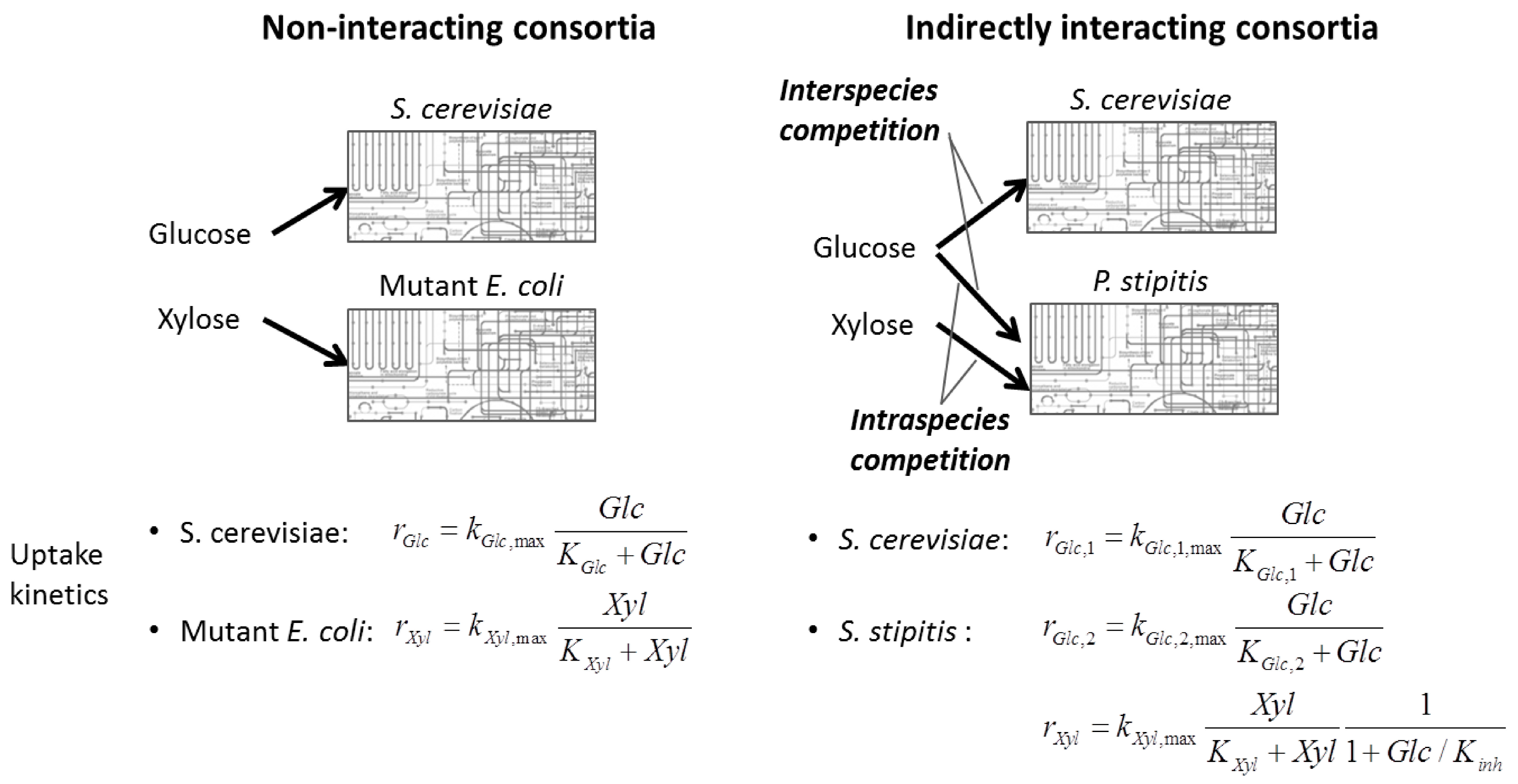
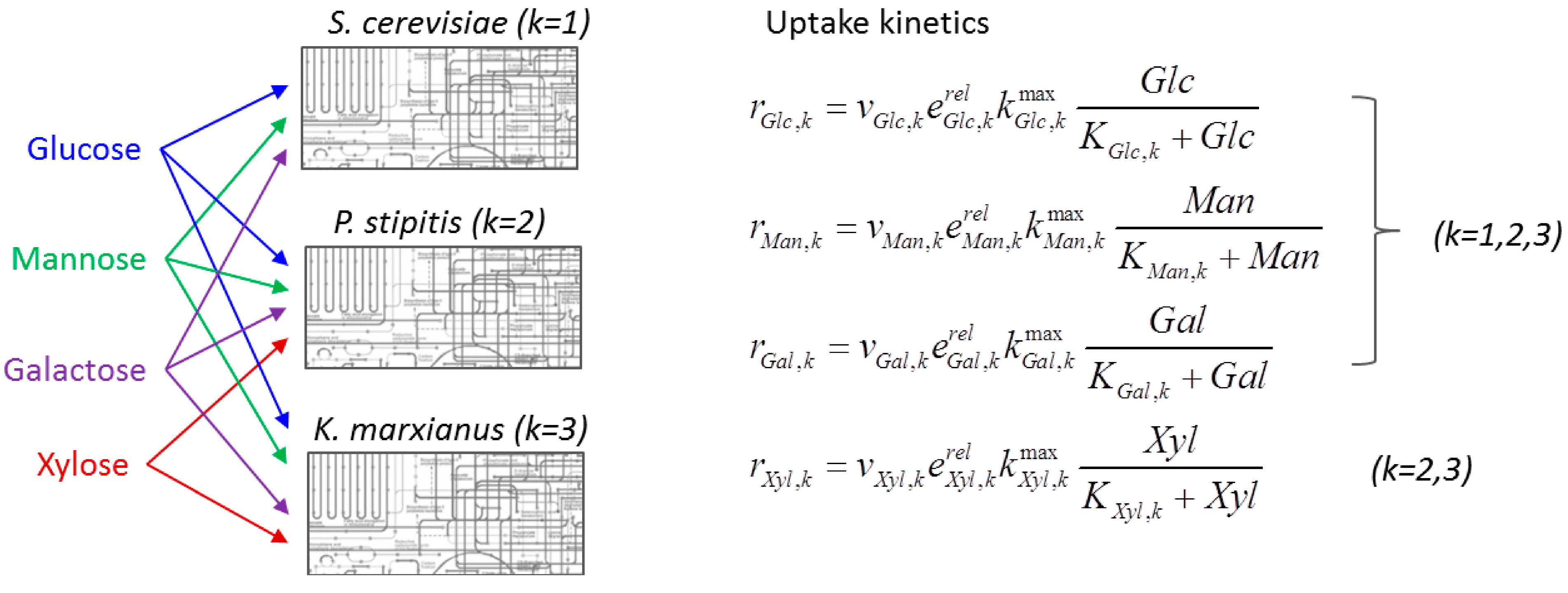
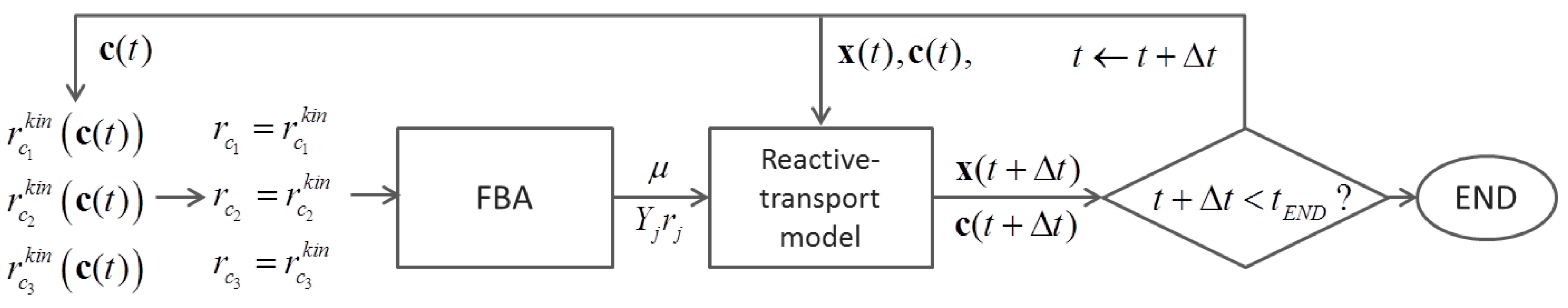
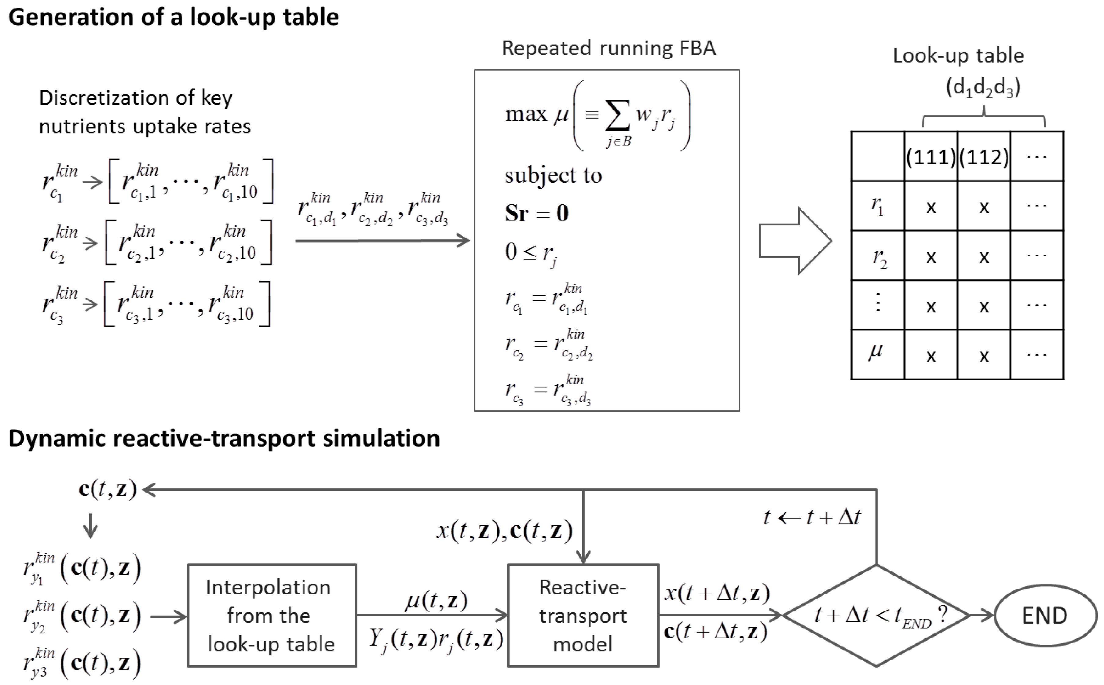
6.2. Indirect Coupling

Model integration is referred to indirect coupling if the outputs obtained from the “independent” simulation of one framework are fed into another model during its simulation. A good example is the integration of a genome-scale network with a reactive transport model by Sheibe et al. [122] for the study of in situ uranium bioremediation by Geobacter species (i.e., Geobacter sulfurreducens). In this system considering a single organism, they repeatedly ran FBA to generate a look-up table that provides the nutrient uptake and growth rates in various possible environmental conditions. Then, the resulting look-up table was referenced at every time step and every grid cell throughout the dynamic simulation of a reactive-transport model. The prediction of condition-specific biomass yield was predicted using FBA by constraining the uptake rates of the three nutrients (acetate, Fe (III), and NH4) that limit the species growth. In order to generate a look-up table, they chose 10 different concentration levels of these key nutrients, and for each of 1000 combinations, they performed FBA. Consequently, they could successfully predict acetate concentration and U (VI) reduction rates in a field trial of in situ uranium bioremediation. Obviously, this indirect coupling results in reduced computation time in comparison to direct coupling that runs both FBA and reactive-transport simulation for their interaction at every time step. As environmental conditions were discretized over coarse meshes, interpolation within the look-up table is required to get the rates between pre-specified conditions. While performing this interpolation process at every time step/grid will be time-consuming, particularly in case of field-scale simulations, one can minimize the look-up table by containing the fluxes of key metabolites only, instead of the full flux vector. Figure 10 illustrates the concept of indirect coupling between FBA and a reactive-transport model. In principle, the same approach can be applied to microbial communities, although the look-up table generation using cFBA and the interpolation would require substantially higher computational power.
Figure 10. Indirect coupling between a reactive-transport model with FBA for the dynamic simulation of a single organism growth. One should first generate a look-up table through the repeated running of FBA with a large number of different sets of nutrient uptake rates (which is 1000 in total in this example) generated by discretizing the range of each uptake (top). During the dynamic simulation of the reactive-transport model, the growth rate and metabolite production rates are updated at each time/location from the look-up table (bottom).
Processes 02 00711 g010
The integration of FBA with dynamic modeling can be considered in a much simpler context—well-mixed conditions—using the framework called dynamic FBA (dFBA) [123]. In a study of bioprocesses that produce bioethanol from glucose and xylose, Hanly and Henson modeled simple consortia composed of two organisms that are (i) non-interacting [124] and (ii) indirectly interacting [125]. The non-interacting consortium was composed of wild-type S. cerevisiae that consumes glucose only and mutated E. coli capable of consuming xylose alone. The indirectly interacting model included (wild-type) S. cerevisiae and Pichia stipites (also known as Scheffersomyces stipitis) that consume both glucose and xylose. In the latter, there were two types of competition–interspecies and intraspecies. While interspecies competition for glucose could be described simply by Michaelis-Menton kinetics, the authors had to incorporate glucose inhibition to describe intraspecies competition between the consumptions of glucose and xylose in P. stipitis (Figure 11). dFBA has also been used in other applications, e.g., for exploring bacterial diversity and their metabolic interactions [126]. In balanced growth conditions where uptake rates change in time but the biomass (and other metabolites) yield from a substrate is constant, the dFBA can be implemented as a form of indirect coupling by referring to the pre-calculation of an FBA solution, without having to solve the LP problem at every time step.
Figure 11. Uptake kinetics for the dynamic FBA (dFBA) simulation of the dynamics of non-interacting (left) and indirectly interacting (right) consortia. Glc and Xyl denote the concentrations of glucose and xylose, respectively. For the sake of simplicity, product (i.e., ethanol) inhibition term is neglected.
Processes 02 00711 g011
Modeling microbial consortia using indirect coupling can also be done by integrating EM analysis with a dynamic framework such as cybernetic models. The framework called hybrid cybernetic model (HCM) [127,128] identifies a relevant subset of EMs as metabolic options for accommodating the metabolic shift in individual species. Geng et al. [129] applied HCM to model a situation where the culture medium contains four sugars (i.e., glucose, xylose, mannose, and galactose) which are competitively consumed by three yeast strains (i.e., S. cerevisiae, P. stipitis, and Kluyveromyces marxianus). Consumption patterns of these sugars vary depending on the organism. S. cerevisiae consumes glucose, mannose, and galactose, but not xylose. Among three hexoses fermentable by S. cerevisiae, galactose is the least preferred substrate, while glucose and mannose are preferably consumed. On the other hand, P. stipitis and K. marxianus ferment all four sugars, the consumption of which starts with the pair of glucose and mannose, followed by the pair of xylose and galactose. Without having to incorporate empirical inhibition terms, the competitive consumption of four sugars by each organism was modeled in a simpler form based on the cybernetic control variables (Figure 12).
The integration of dynamic population-based models (e.g., gLV model) with cFBA would be another possible form of indirect coupling, yet we could not find an appropriate example in the literature. As an input, cFBA requires information of species abundance, the dynamic change of which can be provided from the independent simulation of a gLV model. Thus, this integration enables the prediction of the change of flux distributions at each time step within individual species and the community. These predictions are beyond the level achievable using gLV model or cFBA alone.
Figure 12. Uptake kinetics for the hybrid cybernetic model (HCM) simulation of the consortia composed of three yeast strains (Saccharomyces cerevisiae, Pichia stipitis, and Kluyveromyces marxianus) growing on four different carbon sources. Glc, Man, Gal, and Xyl denote the concentrations of glucose, mannose, galactose, and xylose, respectively. The symbols e and v represent enzyme level and its activity. For the sake of simplicity, self-substrate inhibition term is neglected.
Processes 02 00711 g012

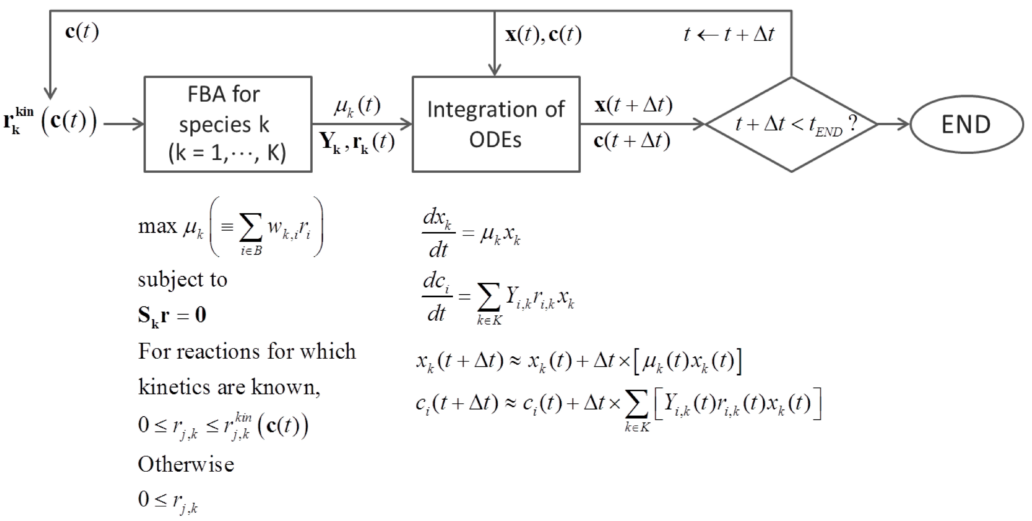
6.3. Direct Coupling

In complex systems containing multiple interacting species and many constraining environmental variables, simulation of microbial community dynamics using look-up tables to indirectly couple FBAs and dynamic models will become unattractive. Fang et al. [130], therefore, applied a “direct” coupling of a genome-scale metabolic network with a reactive-transport model. A reactive-transport model dynamically interacts with FBA at each time step to obtain reaction rates required for solving differential equations (Figure 13).
Figure 13. Implementation of direct coupling between FBA and a reactive-transport model.
Processes 02 00711 g013
In contrast to dFBA-based approaches which assume quasi-steady state on intracellular metabolites, King et al. [131] coupled a reactive transport model with a dynamic model of intracellular kinetics based on a simplified network. Resat et al. [113] also considered intracellular dynamics (using an even simpler network) to describe the cellular dynamics using an IbM framework (similar to BacSim [117]). An IbM was directly coupled with a three dimensional reactive-transport model.
Direct coupling examples addressed above were focused on a single organism, while Resat et al. [113] also considered the simulation of two species. The framework developed by Zhuang et al. [132], on the other hand, demonstrated the extended application of dFBA to ecological settings. Instead of directly obtaining substrate uptake rate as determined by kinetic equations, they use kinetic equations as upper bounds of uptake rates [133]. To simulate the dynamic change of Rhodoferax and Geobacter species, which are acetate oxidizing Fe (III)-reducers competing in anoxic subsurface environments, they identified uptake kinetics for metabolites that affect the growth of species, including acetate, ammonia, and Fe (III) for two species and imposed them as upper bounds in respective FBA implementations. They termed this method as the Dynamic Multispecies Metabolic Modeling (DyMMM) framework. The same method has also been applied to the community of Geobacter and sulfate-reducing bacteria (7SRBs) [134]. Figure 14 shows the procedures of implementing DyMMM.
Figure 14. Implementation of the Dynamic Multispecies Metabolic Modeling (DyMMM) framework proposed by Zhuang et al. [132] for the dynamic simulation of microbial consortia.
Processes 02 00711 g014
Zomorrodi et al. [73] proposed a general framework for the dynamic simulation of microbial community by extending OptCom. In contrast to DyMMM that considers a community-level objective alone, d-OptCom solves a bi-level optimization problem for which both species- and community-level objectives should be specified. d-OptCom also considers uptake kinetics as upper bounds of fluxes, similarly to DyMMM. If species-level objectives are eliminated from the bi-level optimization formulation, the structure between d-OptCom and DyMMM becomes similar while the former solves nonlinear dynamic programming based on an implicit Euler discretization.

7. Summary and Recommendations

So far, we have discussed various forms of mathematical models useful for the analysis and prediction of microbial community dynamics. Table 2 summarizes typical sets of experimental data (or information) for model identification, and inputs and outputs for simulation.
Table 2. An overview of mathematical models discussed throughout the present article. Symbols denote modeling units (_cell: Individual cells, _spe: Species or functional guilds, _tot: Whole community), dependent variables (c: Concentration of extracellular metabolites, e: Abundance of functional genes, rin: Uptake fluxes, r: Full flux vector including intracellular and exchange fluxes, x: Abundance of modeling units) and independent variables (t: Time, z: Spatial location).
ApproachData for Parameter IdentificationInputs for SimulationOutputs from SimulationRemarks
Flux balance analysis (FBA) ([64])N/A (FBA has no parameters to tune)x_spe and rin_tot in a certain conditionr_spe in the given condition
  • Assumes an yield-based (community-level) metabolic objective (such as maximization of biomass yield)
  • Is currently limited to simple consortia
  • Can handle genome-scale metabolic networks
Elementary mode (EM) analysis ([41])N/A (no parameters to tune)Information on x_spe and rin_tot in a certain conditionr_spe in the given condition
  • May not be extended to complex consortia
  • Does not need to specify hypothetical metabolic objective
Gene-centric approach ([42])e_tot(t,z), x_tot(t,z), and c(t,z) upon (designed) perturbationse_tot(0,z), x_tot(0,z), c(0,z) ( i.e., initial distributions)e_tot(t,z), x_tot(t,z), c(t,z), r_tot(t,z) in any new conditions
  • Is applicable to complex communities
  • Does not provide species-level information
Nonlinear regression ([75])x_spe and c across conditions/times/locationsc at a specific condition/ time/locationx_spe in the given condition/time/location
  • Is applicable to large eco-scale settings (such as continents or marines) as well as small scale systems
Trait-based model ([99])x_spe(t) and c(t) upon (designed) perturbationsx_spe(0) and c(0) ( i.e., initial conditions)x_spe(t) and c(t)
  • Simulates the dynamic species-species and species-environment interactions
  • May contain a large number of parameters (to determine)
Generalized Lotka-Volterra (gLV) model ([103])x_spe(t) and c(t) (to model the growth rate as a function of c(t))x_spe(0) and c(0)x_spe(t)
  • Simulates the dynamic change of populations by accounting for interspecies interactions as well as its own growth (in the absence of other species)
Evolutionary game theory ([27])Understanding or knowledge on the interspecies relationshipx_spe(0) and assumed parameter valuesx_spe(t)
  • Models the population to grow/decay by the difference between individual fitness and the community average
  • Is mathematically equivalent to gLV formulation
Thermodynamically-based model ([77])Information on chemical potentials (or reaction rate values)x_spe(0) and c(0)x_spe(∞) and c(∞) ( i.e., values after sufficiently enough time)
  • Predicts the change of species abundance and environmental chemicals by iteratively updating them based on the substrate conversion and microbial growth equations
Population balance model (PBM) ([120])x_spe(t), c(t), and information on population heterogeneityx_spe(0), c(0), and initial population heterogeneityx_spe(t), c(t), and population heterogeneity (evolving with time)
  • Accounts for heterogeneity in populations over external physical and internal state spaces
Individual-based model (IbM) ([113])x_cell(t,z) and c(t,z)x_cell(0,z) and c(0,z)x_cell(t,z) and c(t,z)
  • Simulates emergent behaviors of a community by considering individual cells as discrete autonomous entities
Dynamic FBA (dFBA) ([125])x_spe(t) and c(t)x_spe(0) and c(0)x_spe(t), r_spe(t), and c(t)
  • Couples FBA with kinetics: Nutrient uptake fluxes are given from pre-identified kinetics
Cybernetic model ([129])x_spe(t) and c(t)x_spe(0) and c(0)x_spe(t), r_spe(t), e_spe, and c(t)
  • Assumes a rate-based metabolic objective of species (such as maximization of their uptake rates)
  • Accounts for cellular regulation based on optimal control theory
Dynamic multispecies metabolic modeling (DyMMM) ([132])x_spe(t) and c(t)x_spe(0) and c(0)x_spe(t), r_spe(t), and c(t)
  • Is similar to dFBA, but uses uptake kinetics for setting upper bounds
Dynamic OptCom (d-OptCom) ([73])x_spe(t) and c(t)x_spe(0) and c(0)x_spe(t), r_spe(t), and c(t)
  • Is similar to DyMMM, but flexibly incorporates data and knowledge on species interactions with dual objectives (i.e., at species- and community-levels)
Indirect coupling FBA with transport ([122])x_spe(t,z) and c(t,z)x_spe(0,z) and c(0,z)x_spe(t,z), r_spe(t,z) and c(t,z)
  • Solves a reactive-transport model where nutrient uptake and species growth rates are obtained (at each time and location) by referring to a look-up table (generated through independent FBA simulations)
Based on the work of Song et al. [31], we provide general guidelines for the selection of an appropriate modeling framework (among various candidates) for a given problem. Above all, the choice of a specific model should be based on modeling goals, which can be (i) understanding the characteristics of microbial association under specific settings; (ii) predicting their dynamics in new conditions; (iii) controlling microbial communities to perform desirable functions, or all of them. Then, one may initially consider a couple of candidate frameworks (or more) that could potentially meet modeling goals. For this purpose, it is important to have a sound understanding of the simulation scope of modeling frameworks, for example as summarized in Table 2. Another recommendation is to minimize the complexity of model structure. Therefore, following the principle of Occam’s razor, one would prefer the simplest model (i.e., with the smallest number of parameters and variables) in case that all candidate models perform similarly in data-fitting. Information theoretic tools enable a systematic, quantitative comparison of candidate models in this regard. Statistical merits often used for such comparison include Akiake Information Criterion (AIC) [135] and Bayesian Information Criterion (BIC) [136].

8. Conclusions and Outlook

Considering the complexity of microbial communities, it is not surprising to find a vast number of mathematical tools and frameworks in the literature. The successful application of models will depend on many factors: (i) how flexibly they incorporate computational and experimental tools to improve their predictive power; (ii) how effectively they resolve the problems of academic, industrial, and social interest; and (iii) how significantly they outperform rival models. While one may prefer a specific model to others, it is advantageous to take an integrative approach that selectively combines multiple relevant methods, as discussed in the foregoing section.
Other than the strength of model integration, there are other specific issues that need to be considered in the future modeling efforts. First, while the PBM is a popular framework used for modeling particulate systems, its application to microbial communities is rare. Unless a large number of internal state variables need to be considered for modeling, PBM’s capability to describe population heterogeneity at a reasonable computational cost offers an attractive compromise between population-based models and IbMs. Second, despite the potentially significant role in determining the member interactions and the overall community behavior, the consideration of dynamic metabolic shifts in individual species is limited in current modeling practices. Incorporation of this feature into modeling will make it possible to reveal even richer behavior of microbial communities in response to environmental perturbations as adaptive complex systems. While empirical rules are conceivable for this purpose, mechanistic description of metabolic shift will allow for more realistic predictions across different conditions. In this regard, the incorporation of the cybernetic control laws into population-based models or IbMs is a possible route along the line. Third, ability to leverage increasingly available meta-omics data (e.g., transcriptomic, proteomic, metabolomics data) within the context of community models will improve the prediction accuracy. Finally, an important challenge for the modeling of microbial communities is the ability to encompass different scales. Microbial communities are multiscale systems: The results of microbial community activity at the fine scale can have profound effects on the physical and chemical characteristics at the macroscopic level of an aquatic or terrestrial ecosystem, or a human being. Multiscale modeling has been restricted, however, in practical efforts.
Despite these challenges, the predictive power of microbial community models will grow along with rapid advancement in experimental and computational technologies. Therefore, mathematical models in the future are expected to provide a more profound understanding of microbial community dynamics with an ultimate aim to engineering them.

Acknowledgments

This research was supported by the Genomic Science Program (GSP), Office of Biological and Environmental Research (OBER), U.S. Department of Energy (DOE), and is a contribution of the Pacific Northwest National Laboratory (PNNL) Foundational Scientific Focus Area, the PNNL Biofuels Scientific Focus Area, and Laboratory Directed Research and Development. PNNL is operated by Battelle for the U.S. Department of Energy under Contract DE-AC06-76RLO. The authors thank William C. Nelson at PNNL for valuable discussions on metagenomic analysis.

Author Contributions

All authors contributed to the design of the paper. H.-S.S. and W.R.C. wrote the manuscript, which was edited by A.S.B. and A.K. All authors read and approved the final manuscript.

Conflicts of Interest

The authors declare no conflict of interest.

References

  1. Whitman, W.B.; Coleman, D.C.; Wiebe, W.J. Prokaryotes: The unseen majority. Proc. Natl. Acad. Sci. USA 1998, 95, 6578–6583. [Google Scholar]
  2. Microbiology by numbers. Nat. Rev. Microbiol. 2011, 9, 628. [CrossRef]
  3. Fukuda, S.; Ohno, H. Gut microbiome and metabolic diseases. Semin. Immunopathol. 2014, 36, 103–114. [Google Scholar]
  4. Heintz, C.; Mair, W. You are what you host: Microbiome modulation of the aging process. Cell 2014, 156, 408–411. [Google Scholar] [CrossRef]
  5. Moloney, R.D.; Desbonnet, L.; Clarke, G.; Dinan, T.G.; Cryan, J.F. The microbiome: Stress, health and disease. Mamm. Genome 2014, 25, 49–74. [Google Scholar] [CrossRef]
  6. Maukonen, J.; Saarela, M. Microbial communities in industrial environment. Curr. Opin. Microbiol. 2009, 12, 238–243. [Google Scholar] [CrossRef]
  7. Konopka, A. What is microbial community ecology? ISME J. 2009, 3, 1223–1230. [Google Scholar] [CrossRef]
  8. Bond, P.L.; Smriga, S.P.; Banfield, J.F. Phylogeny of microorganisms populating a thick, subaerial, predominantly lithotrophic biofilm at an extreme acid mine drainage site. Appl. Environ. Microbiol 2000, 66, 3842–3849. [Google Scholar] [CrossRef]
  9. Caporaso, J.G.; Lauber, C.L.; Costello, E.K.; Berg-Lyons, D.; Gonzalez, A.; Stombaugh, J.; Knights, D.; Gajer, P.; Ravel, J.; Fierer, N.; et al. Moving pictures of the human microbiome. Genome Biol. 2011, 12. [Google Scholar] [CrossRef]
  10. Wagg, C.; Bender, S.F.; Widmer, F.; van der Heijden, M.G.A. Soil biodiversity and soil community composition determine ecosystem multifunctionality. Proc. Natl. Acad. Sci. USA 2014, 111, 5266–5270. [Google Scholar] [CrossRef]
  11. Fierer, N.; Lennon, J.T. The generation and maintenance of diversity in microbial communities. Am. J. Bot. 2011, 98, 439–448. [Google Scholar] [CrossRef]
  12. Zengler, K.; Palsson, B.O. A road map for the development of community systems (cosy) biology. Nat. Rev. Microbiol. 2012, 10, 366–372. [Google Scholar]
  13. Haruta, S.; Yoshida, T.; Aoi, Y.; Kaneko, K.; Futamata, H. Challenges for complex microbial ecosystems: Combination of experimental approaches with mathematical modeling. Microbes Environ. 2013, 28, 285–294. [Google Scholar] [CrossRef]
  14. Mee, M.T.; Wang, H.H. Engineering ecosystems and synthetic ecologies. Mol. Biosyst. 2012, 8, 2470–2483. [Google Scholar] [CrossRef]
  15. Larsen, P.; Hamada, Y.; Gilbert, J. Modeling microbial communities: Current, developing, and future technologies for predicting microbial community interaction. J. Biotechnol. 2012, 160, 17–24. [Google Scholar] [CrossRef]
  16. Larsen, P.E.; Gibbons, S.M.; Gilbert, J.A. Modeling microbial community structure and functional diversity across time and space. FEMS Microbiol. Lett. 2012, 332, 91–98. [Google Scholar] [CrossRef]
  17. Kissling, W.D.; Dormann, C.F.; Groeneveld, J.; Hickler, T.; Kuhn, I.; McInerny, G.J.; Montoya, J.M.; Romermann, C.; Schiffers, K.; Schurr, F.M.; et al. Towards novel approaches to modelling biotic interactions in multispecies assemblages at large spatial extents. J. Biogeogr. 2012, 39, 2163–2178. [Google Scholar]
  18. Roling, W.F.M.; van Bodegom, P.M. Toward quantitative understanding on microbial community structure and functioning: A modeling-centered approach using degradation of marine oil spills as example. Front. Microbiol. 2014, 5. [Google Scholar] [CrossRef]
  19. Stegen, J.C.; Lin, X.J.; Konopka, A.E.; Fredrickson, J.K. Stochastic and deterministic assembly processes in subsurface microbial communities. ISME J. 2012, 6, 1653–1664. [Google Scholar] [CrossRef]
  20. Klapper, I.; Dockery, J. Mathematical description of microbial biofilms. SIAM Rev. 2010, 52, 221–265. [Google Scholar] [CrossRef]
  21. Tringe, S.G.; von Mering, C.; Kobayashi, A.; Salamov, A.A.; Chen, K.; Chang, H.W.; Podar, M.; Short, J.M.; Mathur, E.J.; Detter, J.C.; et al. Comparative metagenomics of microbial communities. Science 2005, 308, 554–557. [Google Scholar]
  22. Lidstrom, M.E.; Konopka, M.C. The role of physiological heterogeneity in microbial population behavior. Nat. Chem. Biol. 2010, 6, 705–712. [Google Scholar] [CrossRef]
  23. Majed, N.; Chernenko, T.; Diem, M.; Gu, A.Z. Identification of functionally relevant populations in enhanced biological phosphorus removal processes based on intracellular polymers profiles and insights into the metabolic diversity and heterogeneity. Environ. Sci. Technol. 2012, 46, 5010–5017. [Google Scholar] [CrossRef]
  24. Ramkrishna, D.; Mahoney, A.W. Population balance modeling. Promise for the future. Chem. Eng. Sci. 2002, 57, 595–606. [Google Scholar] [CrossRef]
  25. Hellweger, F.L.; Bucci, V. A bunch of tiny individuals-individual-based modeling for microbes. Ecol. Model. 2009, 220, 8–22. [Google Scholar] [CrossRef]
  26. Scheffer, M.; Baveco, J.M.; Deangelis, D.L.; Rose, K.A.; Vannes, E.H. Super-individuals a simple solution for modeling large populations on an individual basis. Ecol. Model. 1995, 80, 161–170. [Google Scholar] [CrossRef]
  27. Gore, J.; Youk, H.; van Oudenaarden, A. Snowdrift game dynamics and facultative cheating in yeast. Nature 2009, 459, 253–256. [Google Scholar] [CrossRef]
  28. Borenstein, E. Computational systems biology and in silico modeling of the human microbiome. Brief. Bioinform. 2012, 13, 769–780. [Google Scholar] [CrossRef]
  29. Orth, J.D.; Thiele, I.; Palsson, B.O. What is flux balance analysis? Nat. Biotechnol. 2010, 28, 245–248. [Google Scholar]
  30. Trinh, C.T.; Wlaschin, A.; Srienc, F. Elementary mode analysis: A useful metabolic pathway analysis tool for characterizing cellular metabolism. Appl. Microbiol. Biotechnol 2009, 81, 813–826. [Google Scholar] [CrossRef]
  31. Song, H.-S.; DeVilbiss, F.; Ramkrishna, D. Modeling metabolic systems: The need for dynamics. Curr. Opin. Chem. Eng. 2013, 2, 373–382. [Google Scholar] [CrossRef]
  32. Yoo, S.J.; Kim, J.H.; Lee, J.M. Dynamic modelling of mixotrophic microalgal photobioreactor systems with time-varying yield coefficient for the lipid consumption. Biores. Technol. 2014, 162, 228–235. [Google Scholar] [CrossRef]
  33. Urbanczik, R.; Wagner, C. An improved algorithm for stoichiometric network analysis: Theory and applications. Bioinformatics 2005, 21, 1203–1210. [Google Scholar] [CrossRef]
  34. De Figueiredo, L.F.; Podhorski, A.; Rubio, A.; Kaleta, C.; Beasley, J.E.; Schuster, S.; Planes, F.J. Computing the shortest elementary flux modes in genome-scale metabolic networks. Bioinformatics 2009, 25, 3158–3165. [Google Scholar]
  35. Terzer, M.; Stelling, J. Large-scale computation of elementary flux modes with bit pattern trees. Bioinformatics 2008, 24, 2229–2235. [Google Scholar] [CrossRef]
  36. Terzer, M.; Stelling, J. Parallel extreme ray and pathway computation. Lect. Notes Comput. Sci. 2010, 6068, 300–309. [Google Scholar]
  37. Song, H.S.; Ramkrishna, D. Reduction of a set of elementary modes using yield analysis. Biotechnol. Bioeng. 2009, 102, 554–568. [Google Scholar] [CrossRef]
  38. Chan, S.H.J.; Ji, P. Decomposing flux distributions into elementary flux modes in genome-scale metabolic networks. Bioinformatics 2011, 27, 2256–2262. [Google Scholar] [CrossRef]
  39. Ballerstein, K.; von Kamp, A.; Klamt, S.; Haus, U.U. Minimal cut sets in a metabolic network are elementary modes in a dual network. Bioinformatics 2012, 28, 381–387. [Google Scholar] [CrossRef]
  40. Greenblum, S.; Turnbaugh, P.J.; Borenstein, E. Metagenomic systems biology of the human gut microbiome reveals topological shifts associated with obesity and inflammatory bowel disease. Proc. Natl. Acad. Sci. USA 2012, 109, 594–599. [Google Scholar]
  41. Taffs, R.; Aston, J.E.; Brileya, K.; Jay, Z.; Klatt, C.G.; McGlynn, S.; Mallette, N.; Montross, S.; Gerlach, R.; Inskeep, W.P.; et al. In silico approaches to study mass and energy flows in microbial consortia: A syntrophic case study. BMC Syst. Biol. 2009, 3. [Google Scholar] [CrossRef]
  42. Reed, D.C.; Algar, C.K.; Huber, J.A.; Dick, G.J. Gene-centric approach to integrating environmental genomics and biogeochemical models. Proc. Natl. Acad. Sci. USA 2014, 111, 1879–1884. [Google Scholar] [CrossRef]
  43. Ramkrishna, D.; Song, H.S. Dynamic models of metabolism: Review of the cybernetic approach. AIChE J. 2012, 58, 986–997. [Google Scholar] [CrossRef]
  44. Kim, J.I.; Song, H.S.; Sunkara, S.R.; Lali, A.; Ramkrishna, D. Exacting predictions by cybernetic model confirmed experimentally: Steady state multiplicity in the chemostat. Biotechnol. Prog. 2012, 28, 1160–1166. [Google Scholar]
  45. Song, H.S.; Ramkrishna, D. Prediction of metabolic function from limited data: Lumped hybrid cybernetic modeling (l-hcm). Biotechnol. Bioeng. 2010, 106, 271–284. [Google Scholar]
  46. Song, H.S.; Ramkrishna, D. Cybernetic models based on lumped elementary modes accurately predict strain-specific metabolic function. Biotechnol. Bioeng. 2011, 108, 127–140. [Google Scholar] [CrossRef]
  47. Song, H.S.; Ramkrishna, D. Prediction of dynamic behavior of mutant strains from limited wild-type data. Metab. Eng. 2012, 14, 69–80. [Google Scholar] [CrossRef]
  48. Song, H.S.; Ramkrishna, D.; Pinchuk, G.E.; Beliaev, A.S.; Konopka, A.E.; Fredrickson, J.K. Dynamic modeling of aerobic growth of shewanella oneidensis. Predicting triauxic growth, flux distributions, and energy requirement for growth. Metab. Eng. 2013, 15, 25–33. [Google Scholar]
  49. Young, J.D.; Henne, K.L.; Morgan, J.A.; Konopka, A.E.; Ramkrishna, D. Integrating cybernetic modeling with pathway analysis provides a dynamic, systems-level description of metabolic control. Biotechnol. Bioeng. 2008, 100, 542–559. [Google Scholar] [CrossRef]
  50. Faust, K.; Raes, J. Microbial interactions: From networks to models. Nat. Rev. Microbiol. 2012, 10, 538–550. [Google Scholar] [CrossRef]
  51. Shuler, M.L.; Kargi, F. Bioprocess Engineering; Prentice Hall: Upper Saddle River, NJ, USA, 2002. [Google Scholar]
  52. Burmolle, M.; Webb, J.S.; Rao, D.; Hansen, L.H.; Sorensen, S.J.; Kjelleberg, S. Enhanced biofilm formation and increased resistance to antimicrobial agents and bacterial invasion are caused by synergistic interactions in multispecies biofilms. Appl. Environ. Microb. 2006, 72, 3916–3923. [Google Scholar] [CrossRef]
  53. Rodriguez-Martinez, J.M.; Pascual, A. Antimicrobial resistance in bacterial biofilms. Rev. Med. Microbiol. 2006, 17, 65–75. [Google Scholar] [CrossRef]
  54. Pak, K.R.; Bartha, R. Mercury methylation by interspecies hydrogen and acetate transfer between sulfidogens and methanogens. Appl. Environ. Microb. 1998, 64, 1987–1990. [Google Scholar]
  55. Gause, G.F. Experimental studies on the struggle for existence i mixed population of two species of yeast. J. Exp. Biol. 1932, 9, 389–402. [Google Scholar]
  56. Moon, D.C.; Moon, J.; Keagy, A. Direct and indirect interactions. Available online: http://www.nature.com/scitable/knowledge/library/direct-and-indirect-interactions-15650000 (accessed on 11 October 2014).
  57. Berry, D.; Widder, S. Deciphering microbial interactions and detecting keystone species with co-occurrence networks. Front. Microbiol. 2014, 5. [Google Scholar] [CrossRef]
  58. Wooley, J.C.; Godzik, A.; Friedberg, I. A primer on metagenomics. PLOS Comput. Biol. 2010, 6. [Google Scholar] [CrossRef]
  59. Mande, S.S.; Mohammed, M.H.; Ghosh, T.S. Classification of metagenomic sequences: Methods and challenges. Brief. Bioinform. 2012, 13, 669–681. [Google Scholar] [CrossRef]
  60. Fuhrman, J.A. Microbial community structure and its functional implications. Nature 2009, 459, 193–199. [Google Scholar] [CrossRef]
  61. Barabasi, A.L. Scale-free networks: A decade and beyond. Science 2009, 325, 412–413. [Google Scholar] [CrossRef]
  62. Barabasi, A.L.; Bonabeau, E. Scale-free networks. Sci. Am. 2003, 288, 60–69. [Google Scholar] [CrossRef]
  63. Albert, R.; Jeong, H.; Barabasi, A.L. Error and attack tolerance of complex networks. Nature 2000, 406, 378–382. [Google Scholar] [CrossRef]
  64. Stolyar, S.; van Dien, S.; Hillesland, K.L.; Pinel, N.; Lie, T.J.; Leigh, J.A.; Stahl, D.A. Metabolic modeling of a mutualistic microbial community. Mol. Syst. Biol. 2007, 3, 92. [Google Scholar] [CrossRef]
  65. Freilich, S.; Zarecki, R.; Eilam, O.; Segal, E.S.; Henry, C.S.; Kupiec, M.; Gophna, U.; Sharan, R.; Ruppin, E. Competitive and cooperative metabolic interactions in bacterial communities. Nat. Commun. 2011, 2. [Google Scholar] [CrossRef]
  66. Klitgord, N.; Segre, D. Environments that induce synthetic microbial ecosystems. PLOS Comput. Biol. 2010, 6. [Google Scholar] [CrossRef]
  67. Wintermute, E.H.; Silver, P.A. Emergent cooperation in microbial metabolism. Mol. Syst. Biol. 2010, 6. [Google Scholar] [CrossRef]
  68. Segre, D.; Vitkup, D.; Church, G.M. Analysis of optimality in natural and perturbed metabolic networks. Proc. Natl. Acad. Sci. USA 2002, 99, 15112–15117. [Google Scholar] [CrossRef]
  69. Bordbar, A.; Feist, A.M.; Usaite-Black, R.; Woodcock, J.; Palsson, B.O.; Famili, I. A multi-tissue type genome-scale metabolic network for analysis of whole-body systems physiology. BMC Syst. Biol. 2011, 5. [Google Scholar] [CrossRef]
  70. Lewis, N.E.; Schramm, G.; Bordbar, A.; Schellenberger, J.; Andersen, M.P.; Cheng, J.K.; Patel, N.; Yee, A.; Lewis, R.A.; Eils, R.; et al. Large-scale in silico modeling of metabolic interactions between cell types in the human brain. Nat. Biotechnol. 2010, 28, U1279–U1291. [Google Scholar]
  71. Khandelwal, R.A.; Olivier, B.G.; Roling, W.F.M.; Teusink, B.; Bruggeman, F.J. Community flux balance analysis for microbial consortia at balanced growth. PLOS ONE 2013, 8. [Google Scholar] [CrossRef]
  72. Zomorrodi, A.R.; Maranas, C.D. Optcom: A multi-level optimization framework for the metabolic modeling and analysis of microbial communities. PLOS Comput. Biol. 2012, 8. [Google Scholar] [CrossRef]
  73. Zomorrodi, A.R.; Islam, M.M.; Maranas, C.D. D-optcom: Dynamic multi-level and multi-objective metabolic modeling of microbial communities. ACS Synth. Biol. 2014, 3, 247–257. [Google Scholar] [CrossRef]
  74. Elith, J.; Leathwick, J.R. Species distribution models: Ecological explanation and prediction across space and time. Annu. Rev. Ecol. Evol. Syst. 2009, 40, 677–697. [Google Scholar]
  75. Larsen, P.E.; Field, D.; Gilbert, J.A. Predicting bacterial community assemblages using an artificial neural network approach. Nat. Methods 2012, 9, 621–625. [Google Scholar] [CrossRef]
  76. Schmidt, M.; Lipson, H. Distilling free-form natural laws from experimental data. Science 2009, 324, 81–85. [Google Scholar] [CrossRef]
  77. Istok, J.D.; Park, M.; Michalsen, M.; Spain, A.M.; Krumholz, L.R.; Liu, C.; McKinley, J.; Long, P.; Roden, E.; Peacock, A.D.; et al. A thermodynamically-based model for predicting microbial growth and community composition coupled to system geochemistry: Application to uranium bioreduction. J. Contam. Hydrol. 2010, 112, 1–14. [Google Scholar]
  78. Larowe, D.E.; Dale, A.W.; Regnier, P. A thermodynamic analysis of the anaerobic oxidation of methane in marine sediments. Geobiology 2008, 6, 436–449. [Google Scholar] [CrossRef]
  79. Rodriguez, J.; Kleerebezem, R.; Lema, J.M.; van Loosdrecht, M.C.M. Modeling product formation in anaerobic mixed culture fermentations. Biotechnol. Bioeng. 2006, 93, 592–606. [Google Scholar] [CrossRef]
  80. Beard, D.A.; Qian, H. Relationship between thermodynamic driving force and one-way fluxes in reversible processes. PLOS ONE 2007, 2, e144. [Google Scholar] [CrossRef]
  81. Noor, E.; Bar-Even, A.; Flamholz, A.; Reznik, E.; Liebermeister, W.; Milo, R. Pathway thermodynamics highlights kinetic obstacles in central metabolism. PLOS Comput. Biol. 2014, 10, e1003483. [Google Scholar] [CrossRef]
  82. Zhu, Y.; Song, J.; Xu, Z.; Sun, J.; Zhang, Y.; Li, Y.; Ma, Y. Development of thermodynamic optimum searching (tos) to improve the prediction accuracy of flux balance analysis. Biotechnol. Bioeng. 2013, 110, 914–923. [Google Scholar] [CrossRef]
  83. Meysman, F.J.; Bruers, S. Ecosystem functioning and maximum entropy production: A quantitative test of hypotheses. Philos. Trans. R. Soc. B 2010, 365, 1405–1416. [Google Scholar]
  84. Schrödinger, E. What is Life? The Physical Aspect of the Living Cell, 1st ed.; Cambridge University Press: New York, NY, USA, 1944. [Google Scholar]
  85. Prigogine, I. Time, structure, and fluctuations. Science 1978, 201, 777–785. [Google Scholar] [CrossRef]
  86. Morowitz, H.J. Energy Flow in Biology: Biological Organization as a Problem in Thermal Physics; Ox Bow Press: Woodbridge, NJ, USA, 1979. [Google Scholar]
  87. Dewar, R.C. Maximum entropy production and plant optimization theories. Philos. Trans. R. Soc. B 2010, 365, 1429–1435. [Google Scholar] [CrossRef]
  88. Dewar, R.C.; Juretic, D.; Zupanovic, P. The functional design of the rotary enzyme atp synthase is consistent with maximum entropy production. Chem. Phys. Lett. 2006, 430, 177–182. [Google Scholar] [CrossRef]
  89. Unrean, P.; Srienc, F. Metabolic networks evolve towards states of maximum entropy production. Metab. Eng. 2011, 13, 666–673. [Google Scholar] [CrossRef]
  90. Cannon, W.R. Simulating metabolism with statistical thermodynamics. PLOS ONE 2014, 9, e103582. [Google Scholar] [CrossRef]
  91. Schmiedl, T.; Seifert, U. Stochastic thermodynamics of chemical reaction networks. J. Chem. Phys. 2007, 126. [Google Scholar] [CrossRef]
  92. Gillespie, D.T. Stochastic simulation of chemical kinetics. Annu. Rev. Phys. Chem. 2007, 58, 35–55. [Google Scholar] [CrossRef]
  93. Boon, E.; Meehan, C.J.; Whidden, C.; Wong, D.H.J.; Langille, M.G.I.; Beiko, R.G. Interactions in the microbiome: Communities of organisms and communities of genes. FEMS Microbiol. Rev. 2014, 38, 90–118. [Google Scholar] [CrossRef]
  94. Webb, C.T.; Hoeting, J.A.; Ames, G.M.; Pyne, M.I.; Poff, N.L. A structured and dynamic framework to advance traits-based theory and prediction in ecology. Ecol. Lett. 2010, 13, 267–283. [Google Scholar] [CrossRef]
  95. Laughlin, D.C.; Laughlin, D.E. Advances in modeling trait-based plant community assembly. Trends Plant Sci. 2013, 18, 584–593. [Google Scholar] [CrossRef]
  96. Shipley, B.; Vile, D.; Garnier, E. From plant traits to plant communities: A statistical mechanistic approach to biodiversity. Science 2006, 314, 812–814. [Google Scholar] [CrossRef]
  97. Shipley, B.; Paine, C.E.T.; Baraloto, C. Quantifying the importance of local niche-based and stochastic processes to tropical tree community assembly. Ecology 2012, 93, 760–769. [Google Scholar] [CrossRef] [Green Version]
  98. Laughlin, D.C.; Joshi, C.; van Bodegom, P.M.; Bastow, Z.A.; Fule, P.Z. A predictive model of community assembly that incorporates intraspecific trait variation. Ecol. Lett. 2012, 15, 1291–1299. [Google Scholar] [CrossRef]
  99. Jin, Q.S.; Roden, E.E. Microbial physiology-based model of ethanol metabolism in subsurface sediments. J. Contam. Hydrol. 2011, 125, 1–12. [Google Scholar] [CrossRef]
  100. Bouskill, N.J.; Tang, J.; Riley, W.J.; Brodie, E.L. Trait-based representation of biological nitr fication: Model development testing, and predicted community composition. Front. Microbiol. 2012, 3. [Google Scholar] [CrossRef]
  101. Edelstein-Keshet, L. Mathematical Models in Biology; Siam: Philadelphia, PA, USA, 1987; Volume 46. [Google Scholar]
  102. Fisher, C.K.; Mehta, P. Identifying keystone species in the human gut microbiome from metagenomic timeseries using sparse linear regression. Available online: http://arxiv.org/pdf/1402.0511v1.pdf (accessed on 11 October 2014).
  103. Stein, R.R.; Bucci, V.; Toussaint, N.C.; Buffie, C.G.; Ratsch, G.; Pamer, E.G.; Sander, C.; Xavier, J.B. Ecological modeling from time-series inference: Insight into dynamics and stability of intestinal microbiota. PLOS Comput. Biol. 2013, 9. [Google Scholar] [CrossRef]
  104. Mounier, J.; Monnet, C.; Vallaeys, T.; Arditi, R.; Sarthou, A.S.; Helias, A.; Irlinger, F. Microbial interactions within a cheese microbial community. Appl. Environ. Microb. 2008, 74, 172–181. [Google Scholar] [CrossRef] [Green Version]
  105. Nowak, M.A. Evolutionary Dynamics; Harvard University Press: Cambridge, MA, USA, 2006. [Google Scholar]
  106. Nowak, M.A.; Sigmund, K. Evolutionary dynamics of biological games. Science 2004, 303, 793–799. [Google Scholar] [CrossRef]
  107. Frey, E. Evolutionary game theory: Theoretical concepts and applications to microbial communities. Phys. A 2010, 389, 4265–4298. [Google Scholar] [CrossRef]
  108. Minty, J.J.; Singer, M.E.; Scholz, S.A.; Bae, C.H.; Ahn, J.H.; Foster, C.E.; Liao, J.C.; Lin, X.N. Design and characterization of synthetic fungal-bacterial consortia for direct production of isobutanol from cellulosic biomass. Proc. Natl. Acad. Sci. USA 2013, 110, 14592–14597. [Google Scholar] [CrossRef]
  109. Sousa, M.D. Kinetics of distribution of thymus and marrow cells in peripheral lymphoid organs of mouse-ecotaxis. Clin. Exp. Immunol. 1971, 9, 371–380. [Google Scholar]
  110. Kleene, S.J.; Hobson, A.C.; Adler, J. Attractants and repellents influence methylation and demethylation of methyl-accepting chemotaxis proteins in an extract of escherichia-coli. Proc. Natl. Acad. Sci. USA 1979, 76, 6309–6313. [Google Scholar] [CrossRef]
  111. Tindall, M.J.; Maini, P.K.; Porter, S.L.; Armitage, J.P. Overview of mathematical approaches used to model bacterial chemotaxis ii: Bacterial populations. Bull. Math. Biol. 2008, 70, 1570–1607. [Google Scholar] [CrossRef] [Green Version]
  112. Ferrer, J.; Prats, C.; Lopez, D. Individual-based modelling: An essential tool for microbiology. J. Biol. Phys. 2008, 34, 19–37. [Google Scholar] [CrossRef]
  113. Resat, H.; Bailey, V.; McCue, L.A.; Konopka, A. Modeling microbial dynamics in heterogeneous environments: Growth on soil carbon sources. Microb. Ecol. 2012, 63, 883–897. [Google Scholar] [CrossRef]
  114. Tang, Y.N.; Valocchi, A.J. An improved cellular automaton method to model multispecies biofilms. Water Res. 2013, 47, 5729–5742. [Google Scholar] [CrossRef]
  115. Kang, S.; Kahan, S.; Momeni, B. Simulating microbial community patterning using biocellion. In Engineering and Analyzing Multicellular Systems; Springer: Berlin, Germany, 2014; pp. 233–253. [Google Scholar]
  116. Lardon, L.A.; Merkey, B.V.; Martins, S.; Dotsch, A.; Picioreanu, C.; Kreft, J.U.; Smets, B.F. Idynomics: Next-generation individual-based modelling of biofilms. Environ. Microbiol. 2011, 13, 2416–2434. [Google Scholar] [CrossRef]
  117. Kreft, J.U.; Booth, G.; Wimpenny, J.W.T. Bacsim, a simulator for individual-based modelling of bacterial colony growth. Microbiol.-UK 1998, 144, 3275–3287. [Google Scholar] [CrossRef]
  118. Ramkrishna, D. Population Balances: Theory and Applications to Particulate Systems in Engineering; Academic Press: Pittsburgh, PA, USA, 2000. [Google Scholar]
  119. Henson, M.A. Dynamic modeling of microbial cell populations. Curr. Opin. Biotechnol. 2003, 14, 460–467. [Google Scholar] [CrossRef]
  120. Shu, C.C.; Chatterjee, A.; Dunny, G.; Hu, W.S.; Ramkrishna, D. Bistability versus bimodal distributions in gene regulatory processes from population balance. PLOS Comput. Biol. 2011, 7. [Google Scholar] [CrossRef]
  121. Fernandes, R.L.; Nierychlo, M.; Lundin, L.; Pedersen, A.E.; Tellez, P.E.P.; Dutta, A.; Carlquist, M.; Bolic, A.; Schapper, D.; Brunetti, A.C.; et al. Experimental methods and modeling techniques for description of cell population heterogeneity. Biotechnol. Adv. 2011, 29, 575–599. [Google Scholar]
  122. Scheibe, T.D.; Mahadevan, R.; Fang, Y.L.; Garg, S.; Long, P.E.; Lovley, D.R. Coupling a genome-scale metabolic model with a reactive transport model to describe in situ uranium bioremediation. Microb. Biotechnol. 2009, 2, 274–286. [Google Scholar] [CrossRef]
  123. Mahadevan, R.; Edwards, J.S.; Doyle, F.J. Dynamic flux balance analysis of diauxic growth in escherichia coli. Biophys. J. 2002, 83, 1331–1340. [Google Scholar] [CrossRef]
  124. Hanly, T.J.; Henson, M.A. Dynamic flux balance modeling of microbial co-cultures for efficient batch fermentation of glucose and xylose mixtures. Biotechnol. Bioeng. 2011, 108, 376–385. [Google Scholar] [CrossRef]
  125. Hanly, T.J.; Henson, M.A. Dynamic metabolic modeling of a microaerobic yeast co-culture: Predicting and optimizing ethanol production from glucose/xylose mixtures. Biotechnol. Biofuels 2013, 6. [Google Scholar] [CrossRef]
  126. Tzamali, E.; Poirazi, P.; Tollis, I.G.; Reczko, M. A computational exploration of bacterial metabolic diversity identifying metabolic interactions and growth-efficient strain communities. BMC Syst. Biol. 2011, 5. [Google Scholar] [CrossRef]
  127. Kim, J.I.; Varner, J.D.; Ramkrishna, D. A hybrid model of anaerobic e. Coli gjt001: Combination of elementary flux modes and cybernetic variables. Biotechnol. Progr. 2008, 24, 993–1006. [Google Scholar]
  128. Song, H.S.; Morgan, J.A.; Ramkrishna, D. Systematic development of hybrid cybernetic models: Application to recombinant yeast co-consuming glucose and xylose. Biotechnol. Bioeng. 2009, 103, 984–1002. [Google Scholar] [CrossRef]
  129. Geng, J.; Song, H.S.; Yuan, J.Q.; Ramkrishna, D. On enhancing productivity of bioethanol with multiple species. Biotechnol. Bioeng. 2012, 109, 1508–1517. [Google Scholar] [CrossRef]
  130. Fang, Y.L.; Scheibe, T.D.; Mahadevan, R.; Garg, S.; Long, P.E.; Lovley, D.R. Direct coupling of a genome-scale microbial in silico model and a groundwater reactive transport model. J. Contam. Hydrol. 2011, 122, 96–103. [Google Scholar] [CrossRef]
  131. King, E.L.; Tuncay, K.; Ortoleva, P.; Meile, C. In silico geobacter sulfurreducens metabolism and its representation in reactive transport models. Appl. Environ. Microb. 2009, 75, 83–92. [Google Scholar] [CrossRef]
  132. Zhuang, K.; Izallalen, M.; Mouser, P.; Richter, H.; Risso, C.; Mahadevan, R.; Lovley, D.R. Genome-scale dynamic modeling of the competition between rhodoferax and geobacter in anoxic subsurface environments. ISME J. 2011, 5, 305–316. [Google Scholar] [CrossRef]
  133. Harcombe, W.R.; Riehl, W.J.; Dukovski, I.; Granger, B.R.; Betts, A.; Lang, A.H.; Bonilla, G.; Kar, A.; Leiby, N.; Mehta, P.; et al. Metabolic resource allocation in individual microbes determines ecosystem interactions and spatial dynamics. Cell Rep. 2014, 7, 1104–1115. [Google Scholar]
  134. Zhuang, K.; Ma, E.; Lovley, D.R.; Mahadevan, R. The design of long-term effective uranium bioremediation strategy using a community metabolic model. Biotechnol. Bioeng. 2012, 109, 2475–2483. [Google Scholar] [CrossRef]
  135. Akaike, H. Information theory and an extension of the maximum likelihood principle. In Proceedings of the 2nd International Symposium on Information Theory; Akadémiai Kiadó: Budapest, Hungary, 1973; pp. 267–281. [Google Scholar]
  136. Schwarz, G. Estimating the dimension of a model. Ann. Stat. 1978, 6, 461–464. [Google Scholar] [CrossRef]

