Unrestricted Horizon Predictive Controller Applied in a Biphasic Oil Separator under Periodic Slug Disturbances

Abstract

Multi-phase flow, characterised by the presence of both liquid and gas phases, often occurs in riser pipes during oil extraction. These flows can be problematic because they can cause oscillations due to the formation of bubbles within the pipes, which can negatively impact the safety and efficiency of offshore production operations. One solution to this problem is to use a gravitational oil separator, which is designed to dampen these oscillations. The separator is equipped with a control system that uses liquid level and gas pressure sensors to stabilise the flow by adjusting the positions of its valves. This paper presents the use of a specific type of model-based predictive controller to control the level and pressure of a biphasic oil separator, particularly in the presence of slug disturbances. The designs of the separator model and controller are discussed in detail, with a focus on the advantages of using an unrestricted horizon predictive controller, such as its ability to make predictions over a long horizon and its relatively low computational requirements. For the sake of comparison, a linear quadratic regulator is also evaluated. The simulation results demonstrate that the proposed control system is able to effectively regulate the separator’s liquid level and gas pressure within a magnitude range of ${10}^{-4}$ m for the liquid level and ${10}^{-3}$ bar for the internal pressure. Aside from that, the dynamics of the closed-loop system is six times faster than the plant’s for the liquid behaviour and 30 times faster for the pressure, while also presenting sharp attenuation characteristics for the input disturbances of nearly 50 dB for the pressure output and 68 dB for the liquid level.

1. Introduction

In offshore oil production, a multi-phase mixture of oil, gas and water is transported from the seabed wells through submarine risers to the surface and onto a platform. The initial piece of equipment on the platform is the separator, which not only separates but also minimises oscillation in the incoming mixture flow to ensure optimal efficiency for the remaining platform equipment.

As an example, the oil production in Brazil is based mostly on offshore pre-salt exploration. For this, several challenges must be faced which are related to exploration in increasingly deep waters. In addition, the control and optimisation of processes is essential for the smooth functioning and financial return of projects with high investments, as is the pre-salt layer case. Deep water well existence further and further away from the shore generates piping lines (risers) of large extensions and of different geometries. Because of this, the occurrence of irregular flows with severe oscillations in pressure and flow rate, known as slug flow, becomes recurrent, causing operational problems during production. Low efficiency in primary separation, overflow in the separators and reduced equipment life are among the possible problems caused by flows of this type.

Reducing the opening of the surface choke valve, through which oil comes from the wells, is a direct solution to this problem. However, this considerably decreases the production rate, especially in fields where pressure is lower, in addition to possible back pressure problems in wells. Thus, it is necessary to find alternatives that guarantee a stable flow with high productivity. Therefore, an alternative is to reduce part of this oscillation to the primary processing plants on the platform by using control strategies to stabilise the slugs. In this scenario, the gravitational separator is, in general, the first piece of equipment in production processing and should be responsible for stabilising these oscillations. According to Stewart and Arnold [1], in order to obtain a separator design suitable for surface production facilities, it is essential to maintain the quality and quantity of the produced hydrocarbon fluids and to avoid major operational problems in the downstream equipment.

In oil and gas separators, the gas and liquid at a specific temperature and pressure are separated from a hydrocarbon stream, and therefore their design, structure, and operation are critical [1]. Some minimum requirements exist for the design process for gas–liquid separators used in oil and gas processing plants [2]. Research on separators as a novel gas–liquid separator on offshore platforms [3] is evident nowadays. Additionally, the flow behaviour of crude oil in a battery (several separators operating at different pressures) of industrial crude oil and gas separators in the oil industry has been studied [4], as well as the evaluation of flow characteristics in an onshore horizontal separator using computational fluid dynamics [5].

Some studies addressed the basis of two-phase separator design selection and explored the applicability of artificial neural networks for the creation of intelligent systems to predict proper separator dimensions or an evolutionary computational approach in the design of horizontal gravity separators [6,7,8]. Other works analysed separator performance, such as for corrugated plate gas–liquid separators [9], horizontal multi-pipe separators (for subsea oil–water bulk separation) [10], and gas–liquid cylindrical cyclone separators [11]. Additionally, the design and capital cost optimisation of gravity separators were studied [12].

Oscillations in production are often called intermittent or slug flow and are characterised by a cyclic behaviour causing flow and pressure oscillations [13]. These conditions cause numerous operational problems in oil production, such as reductions in the lifespan of the equipment, reducing primary separation efficiency, separator overflow, burning gas to decrease the pressure inside separator, and in the worst case, emergency platform shutdowns [14].

Research on the cause and modelling of slugs is presented in the literature. For instance, Cozin et al. [15] showed that a two-phase slug flow might be characterised using artificial neural networks. A correlation between the phase velocity in the slug body and overall superficial flow velocity is built based on a slug closure model [16]. Mathematical models and numerical methods to study the inner flow field in oil–water disc separators aiming to optimise their design were presented in [17,18]. Aiming at dampening slug-induced oscillatory disturbances in the inflow to the gravity separator, slug handling with a virtual harp based on nonlinear predictive control for a gravity separator was presented in [19]. Aside from that, slugging frequency correlation was analysed for inclined gas–liquid flow in [20], where a novel correlation for the slugging frequency in inclined gas–liquid flow is proposed through experimental data, with the results suggesting that the liquid superficial velocity significantly influences the frequency for the range of flow conditions studied. Additionally, the vertical pipe properties, as characteristics of slug and churn turbulence, under varying flow parameters can be effectively understood using cross-nonlinear analysis, offering a new perspective for analysing the spatiotemporal evolution, instability, and complexity in oil–gas–water three-phase flow [21].

The conventional solution to reduce slug flow effects is to control the choke valve. However, this causes a back pressure increase in oil wells and decreases the production rate, and some solutions have been proposed to ensure stable flow and maximum oil production [22,23]. The feedback control loop is the most used method in the literature to manipulate the valves of separators. It is possible to implement a strategy to keep the level and pressure in the separator within a safe range of operation, increasing separation and reducing flow oscillations in the downstream equipment [24,25]. A control strategy letting the separator level oscillate within certain limits or bands was presented in [26]. As can be noticed, the most commonly used control technique is still the proportional–integral–derivative (PID) and its derivations.

The main aim of the feedback loop in a gravitational oil separator is to absorb disturbances from the input flow, keeping the pressure and level variables in acceptable value ranges. Nunes [27] proposed a control model based on bands, which allows the level to oscillate within certain limits. This control is based on direct level measurement instead of flow measurement, obtaining a simpler and better performance model. Matrix modelling of systems using state variables is the most efficient way to represent multiple-input multiple-output (MIMO) systems, in addition to being necessary for the modern control method’s application. Minghui and Gensheng [28] described the temperature profile in a well through state spaces. Through this representation, it is possible to analyse the thermal behaviour during the circulation and closing phases, making it possible to propose control techniques for the temperature. The linear quadratic regulator (LQR) is an efficient modern control method which uses a cost function to optimise the controller. Liu et al. [29] proposed a control strategy to reduce the problem of riser recoil in deep waters, using the LQR, some results are obtained, reducing risks during operation. The LQR was also used in other publications for optimal damping stabilisation [30], singularly perturbed systems [31], linear system switching [32], and optimal reference tracking for three-phase separators [33].

Despite the amount of research that uses classical and modern control strategies, the implementation of predictive controllers in gravity separators is gaining prominence. Model-based predictive control (MPC) is a technique that uses optimisation (such as LQR) and still regards the so-called prediction horizon to determine the action plan from k (current time) until $N_y$ (future fixed horizon). MPC’s ability to anticipate future events and implement control actions accordingly, as well as its natural ability to deal with constraints, are the main keys to its success in several industry applications [34].

One of the first investigations on MPC in gravity separators was carried out by Stokke et al. [35]. The authors compared MPC with linear–quadratic–Gaussian (LQG) control and stated that the first was superior in performance. For instance, LQG control presented more sensitivity to noise. The prediction horizon was selected to be 30 samples, with a sampling time of 2 s. Notice that in this case, the prediction horizon was only 60 s, whilst the system’s settling time was about 100 s. On the other hand, expanding the prediction horizon would increase further the computational cost, which was an issue for the authors. Mendes et al. [36] showed the implementation of nonlinear MPC (NMPC) in a three-phase oil separator. The performance of the proposed strategy was compared with a traditional PI controller used in the industry. The obtained comparative results showed that NMPC gave the better results, allowing good oscillation attenuation under slug perturbations. However, the prediction horizon was only set to 20 samples with a sampling time of 10 s, giving only 200 s of prediction within a model that needs several hours for settling. Likewise, Hansen et al. [37] used MPC for a three-phase gravity separator, with a comparison with $H_{\infty }$ control. The authors cited that by applying the MPC solution, the gravity separator volume can be used as a buffer for the inflow and keep the level within the constraints under more severe conditions than the compared $H_{\infty }$ control solution. The prediction horizon was set to 600 samples with a sampling time of 0.2 s (120 s of prediction). Jespersen and Yang [38] present a study where they compare a PID, an $H_{\infty }$ control and a MPC for the control of a three phase oil separator. Experimental results based on a lab-scaled pilot plant illustrate the huge potential and benefit of the MPC to significantly improve the effluent water quality, particularly when the process is subject to slugging inflow. Here, the prediction horizon is also set to 600 samples with a sampling time of 0.2 s.

It is interesting to remark that the MPC prediction horizons of the cited works increased with the available computational power. Nevertheless, none of the cited papers used a prediction horizon near the plant settling time, which would be the optimal case according to the literature [39]. This happened due to the increased computational cost. The size of the MPC signal vector, which must be solved at every time step, is given by $z{N}_y$ [40], with $N_y$ being the prediction horizon (in samples) and z being the order of the plant. We remark that the implementation of increased-size matrices and vectors into actual microprocessors is a challenge mainly due to the sampling time. Larger vectors or matrices require more processing time, and generally, the smaller the required sampling time for such calculations, the more expensive the microprocessor is. An interesting example of this drawback was cited by Backi et al. [19]. The authors stated that they recognised that real-time applicability is a crucial aspect of MPC implementation. To provide a comprehensive analysis, they utilised a detailed model that included droplet calculations for oil in water and water in oil. Nevertheless, the use of simpler linear models may be considered an option to reduce the computational time in actual applications. Additionally, Riberio et al. [41] presented a work where the existing offshore production system models, as described in the literature, underwent modifications to increase their usefulness and realism in the context of advanced control studies. The authors conducted a case study on a real plant to quantify the well-known benefits of MPC. The findings highlight MPC’s ability to maintain quality despite perturbations, its intelligent and adaptive set point selection in response to economic considerations and perturbations, and its secure operation without constraint violations, even under perturbations. However, the computation cost of the algorithm is high. Therefore, to ensure computational efficiency, they modified the plant model to maintain cost-effectiveness.

It can be seen that despite the fact few works exist with MPC implementation for control of the level and pressure in oil separators, there are several papers which coped with MPC performing higher-level tasks on petroleum production platforms, such as the works of Neto and Secchi [42], Godhavn et al. [22], Campos et al. [43], and Willersrud et al. [44]. The convergence point of these four works, among others, is the use of MPC mainly for the supervision layer, where both higher sampling times and simplified models can easily be used. Differently, when using MPC for the primary control, the computation cost takes its toll, increasing the processing time and preventing high-frequency implementations of the algorithm.

Controversially, there are two light computing MPC models that reduce dramatically the computational cost in comparison with the most common ones (generalised predictive controller and dynamic matrix controller (GPC and DMC, respectively)). The predictive functional controller (PFC) was developed by Richalet et al. in 1978 [45]. It counts with a control algorithm which does not require any matrix inversion or numerical minimisation of a cost function, and it can be realised for transfer function models. For multivariable processes, one interesting light computing MPC model is the so-called unrestricted horizon predictive controller (UHPC) for SISO and MIMO cases [46,47]. Such a controller is applied for pitch control in a grid-connected wind turbine. In spite of the challenges of the plant model size and controller’s sampling time, the UHPC reduces the computational cost, making it a preferable choice for power system applications [48]. Furthermore, the UHPC is used to ensure stability, robustness, reference tracking, and disturbance rejection even in the presence of modelling errors and noise in a continuous stirred tank reactor (CSTR), where greater margins of stability and noise attenuation are obtained in comparison with the GPC, being able to maintain the same loop response throughout the control system’s operating range without degrading the performance of the controller, which is not the case with the GPC [49].

The UHPC might be a compelling option for the current oil industry. Its calculated matrices do not increase with $N_y$ but solely with the order of the plant. In other words, it is possible to use small sampling times and long prediction horizons without overloading the computational cost, facilitating implementation in a microcontroller. Given that there are still no published works on UHPCs applied to gravity separators, the authors considered investigating, in this paper, the possibility of its implementation in a simulation environment, aiming to reduce level and pressure oscillations caused by slugs.

Section 2 presents both the process and slug modellings (Section 2.1) and the UHPC equating and design for the proposed plant (Section 2.2). Section 3 shows computer simulations of the proposed control strategy applied to a gravity two-phase separator, where four different simulation scenarios are studied: open loop, closed loop with input disturbances as slugs, closed loop for a reference change in the liquid level, and frequency response for the open- and closed-loop cases. Finally, the discussions and conclusions are presented in Section 4.

2. Materials and Methods

This section presents the modelling of the biphasic oil separator, detailing its nonlinear differential equations and the constant values used in this work. In addition, this section presents the UHPC and its equating and design for the closed-loop system, aimed at damping the slug disturbances.

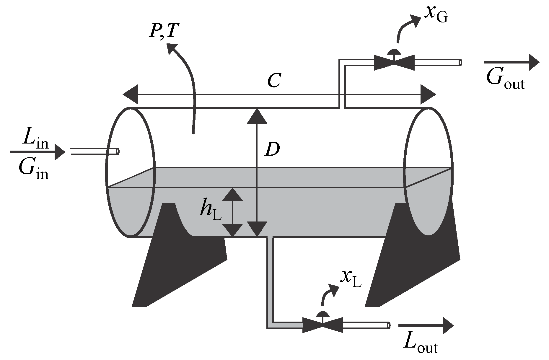
2.1. Modelling of the Biphasic Oil Separator

During the extraction of oil from offshore locations, a phenomenon known as multiphase flow occurs in the riser pipes. This is a mixture of water, oil, and gas that exhibits an oscillatory behaviour. The flow of gas and liquid in these pipes often occurs in bursts, which can disrupt various processes in the production chain of these offshore platforms. This flow is caused by the formation of elongated gas bubbles within vertical lift ducts. These bubbles have a shape similar to projectiles, known as Taylor bubbles, which is depicted in Figure 1. The bubbles occupy almost the entire diameter of the tube, attached to a liquid thin sheet that slides through the tube. This blade has a slower speed than the bubbles and may even have a direction contrary to the flow in certain sections of the tube [50].

As the primary focus of this extraction is economic gain through the production of hydrocarbons (oil and gas), it is necessary to equip these fields (both maritime and terrestrial) with appropriate production facilities. These facilities are specifically designed to carry out the primary processing of these fluids [51].

At a primary processing facility, the first step is to separate the gas, which is less dense, from the liquids through gravitational forces. This process occurs in the initial stage, known as the two-phase separator, which is divided into two sections: the primary section and the secondary section. In the primary section, the fluid collides with deflectors that abruptly change its speed and direction, directing the liquid elements to the bottom of the reservoir. In the secondary section, the larger oil droplets present in the gaseous phase are allowed to settle out. However, the gaseous flow still holds some oil particles that are captured through porous means in the coalescence section, which is typically located near the gas outlet valve [1].

The separator typically consists of a cylindrical tank where a mixture of oil and dissolved gas enters and separates through the process inside the tank. The gas and oil then exit through the upper and lower valves, respectively. The pressure inside the tank and the oil level are the variables that are typically controlled in this process. This work assumes liquid incompressibility (constant density) and an isothermal process, and the gas is assumed to be inert or ideal. Figure 2 illustrates a schematic representation of the described system. In the figure, $L_{\mathrm{in}}$, $L_{\mathrm{out}}$, $G_{\mathrm{in}}$, and $G_{\mathrm{out}}$ are the inflows and outflows of liquid and gas (m${}^3$/s), respectively, C is the separator length (m), D is its diameter (m), $h_L$ is the liquid level (m), P and T are the pressure (bar) and temperature (K) inside the separator, respectively, and $x_L$ and $x_G$ are the liquid and gas valve opening values, respectively, given from 0 (completely closed) to 1 (completely open).

The outlet liquid $L_{\mathrm{out}}$ and gas $G_{\mathrm{out}}$ flows adopt expressions for linear valves commonly used in the industry [52], such as

$$\begin{array}{cc}\hfill L_{\mathrm{out}}\left(t\right)& =2.4·{10}^{-4}{x}_L\left(t\right)C_{V_L}\sqrt{\frac{P\left(t\right)+({\rho }_{L}g{h}_L\left(t\right)·{10}^{-5})-P_1}{{\rho }_L/{\rho }_{H_{2}O}}},\hfill \end{array}$$

(1)

$$\begin{array}{cc}\hfill G_{\mathrm{out}}\left(t\right)& =2.4·{10}^{-4}{x}_g\left(t\right)C_{V_g}\sqrt{\frac{\left(P\left(t\right)-P_2\right)T\left(P\left(t\right)+P_2\right){\left(Mm\right)}_0}{{\left(Mm\right)}_g/P{\left(t\right)}^2}},\hfill \end{array}$$

(2)

with g being the gravitational acceleration (m/s${}^2$), $C_{V_L}$ and $C_{V_g}$ being the flow coefficients of the liquid and gas valves (gpm/psi), respectively, ${\rho }_L$ and ${\rho }_{H_{2}O}$ being the liquid and water densities (kg/m${}^3$), respectively, $P_1$ and $P_2$ being the downstream pressures of the liquid and gas valves (bar), respectively, and ${\left(Mm\right)}_0$ and ${\left(Mm\right)}_g$ being the molar masses of air and gas (kg/mol), respectively.

Nunes et al. [51] showed that the equation for determining the volume of liquid within a two-phase cylindrical separator based on its geometric features, shown in Figure 2, is as follows:

$$\begin{array}{c}\hfill V_L\left(t\right)=\frac{D^{2}C}{4}\left(arccos\left(\frac{D-2h_L\left(t\right)}{D}\right)-\frac{2h_L\left(t\right)\left(D-2h_L\left(t\right)\right)\sqrt{D-h_L\left(t\right)}}{D^2}\right).\end{array}$$

(3)

The same reference gives the equations for the liquid and gas balances inside the gravity separator as follows:

$$\begin{array}{cc}\hfill \frac{d{h}_L\left(t\right)}{dt}& =\frac{L_{\mathrm{in}}\left(t\right)-L_{\mathrm{out}}\left(t\right)}{2C\sqrt{h_L\left(t\right)(D-h_L\left(t\right))}},\hfill \end{array}$$

(4)

$$\begin{array}{cc}\hfill \frac{dP\left(t\right)}{dt}& =\frac{P\left(t\right)\left(G_{\mathrm{in}}\left(t\right)-G_{\mathrm{out}}\left(t\right)+L_{\mathrm{in}}\left(t\right)-L_{\mathrm{out}}\left(t\right)\right)}{V-V_L\left(t\right)},\hfill \end{array}$$

(5)

with V being the total volume of the separator (m${}^3$).

Finally, typical slug liquid and gas flow inputs that may be simplified to sine waves with a period of 2800 s are summed to their mean values ($\overline{L_{\mathrm{in}}}$ and $\overline{G_{\mathrm{in}}}$, respectively) as follows [51]:

$$\begin{array}{cc}\hfill L_{\mathrm{in}}\left(t\right)& =\overline{L_{\mathrm{in}}}+0.082sin\left(\frac{2\pi t}{2800}\right),\hfill \end{array}$$

(6)

$$\begin{array}{cc}\hfill G_{\mathrm{in}}\left(t\right)& =\overline{G_{\mathrm{in}}}+0.075sin\left(\frac{2\pi t}{2800}\right).\hfill \end{array}$$

(7)

Table 1. Biphasic oil separator constants.

Symbol	Description	Value	Unity
$C_{V_L}$	Liquid valve flow coefficient	1025	gpm/psi
$C_{V_g}$	Gas valve flow coefficient	120	gpm/psi
${\rho }_L$	Liquid density	850	kg/m${}^3$
${\rho }_{H_{2}O}$	Water density	999.19	kg/m${}^3$
$P_1,P_2$	Valves downstream pressure	6	bar
T	Separator internal temperature	303.15	K
${\left(Mm\right)}_0$	Air molar mass	0.039	kg/mol
${\left(Mm\right)}_g$	Gas molar mass	0.021	kg/mol
D	Separator diameter	3	m
C	Separator length	8	m
V	Separator volume	56.55	m${}^3$

shows the constants of the separator model to be used in this work, whilst

Table 2. Biphasic oil separator steady state values.

Symbol	Description	Value	Unity
$\overline{x_L}$	Liquid valve opening	0.4375	1
$\overline{x_G}$	Gas valve opening	0.0536	1
$\overline{L_{\mathrm{in}}}$	Liquid flow inlet	0.165	m${}^3$/s
$\overline{L_{\mathrm{out}}}$	Liquid flow outlet	0.165	m${}^3$/s
$\overline{G_{\mathrm{in}}}$	Gas flow inlet	0.1	m${}^3$/s
$\overline{G_{\mathrm{out}}}$	Gas flow outlet	0.1	m${}^3$/s
$\overline{h_L}$	Internal liquid level	2	m
$\overline{P}$	Internal pressure	8	bar
$\overline{V_L}$	Volume of liquid	40.05	m${}^3$

presents its steady state values.

The two-phase oil separator nonlinear model presented in this section in Equations (1)–(7) is used for numeric simulations in Section 3, in addition to being used for the controller design after linearization in the following section.

2.2. The Unrestricted Horizon Predictive Controller

This section exploits the unrestricted horizon predictive controller (UHPC) and its equating and design for controlling the gravitational oil separator, which were presented previously.

The reader should note that the UHPC fits into the category of model-based predictive control (MPC). These type of controllers have been developed to address some of the limitations of traditional controllers, such as the input-output constraints, wind-up effect, and optimisation of control objectives [34]. The natural behaviour of MPC and its well-posed mathematical approach to dealing with constraints has led to it being widely accepted in both academia and industry [39].

Perhaps the most known and implemented MPC model is the generalised predictive controller (GPC), which was first presented by Clarke et al. [40]. Nevertheless, without its stochastic potential—which is rarely used—the GPC becomes similar to the predictive functional controller (PFC). The PFC is perhaps the most known member of the low computing cost MPC family [34]. The main difference between them is that the GPC is a multivariable controller, whilst the PFC is essentially a SISO one, therefore not being suitable for the application presented in this paper. Among these two MPC approaches lies the UHPC, which features stochasticity, multivariability, and a low computing cost. We also note that the UHPC is a general usage linear MPC model [46,47] such that its presented design does not aim at any specific application.

2.2.1. UHPC Equating

In contrast to traditional MPC models, the UHPC, similar to the PFC, utilises a quadratic cost function that considers only a single point in the future. For the general discrete state space system given by

$$\begin{array}{cc}\hfill \mathit{x}(k+1)& =\mathbf{A}\mathit{x}\left(k\right)+\mathbf{B}\mathit{u}(k-d)+\Gamma \mathbf{\xi }\left(k\right),\hfill \end{array}$$

(8)

$$\begin{array}{cc}\hfill \mathit{y}\left(k\right)& =\mathbf{C}\mathit{x}\left(k\right)+\mathbf{\xi }\left(k\right),\hfill \end{array}$$

(9)

this cost is defined as

$$\begin{array}{c}\hfill \mathcal{J}=\mathit{x}{(k+N_y)}^T\mathbf{Q}\mathit{x}(k+N_y)+\mathit{u}{\left(k\right)}^T\mathbf{R}\mathit{u}\left(k\right),\end{array}$$

(10)

subjected to the diagonal weighting matrices $\mathbf{Q}={\mathbf{Q}}^T\ge 0$ and $\mathbf{R}={\mathbf{R}}^T\ge 0$. $\mathbf{A}$, $\mathbf{B}$, $\mathbf{C}$, and $\Gamma$ are the state, input, output, and disturbance matrices in discrete form, respectively, while $\mathit{x}$, $\mathit{u}$, and $\mathbf{\xi }$ are the system state and input and noise vectors, respectively, and d is the transport delay.

Notice that regarding a single future point $N_y$ means that any information between k and $N_y$ is neglected by the UHPC during optimisation for the control law calculation. In practice, it implies that the UHPC calculates the control law, looking only to point $N_y$ ahead. By doing so at every time step, the prediction window is entirely swept in $N_y$ steps. Thus, the UHPC regards that if the system remains stable at sample time $N_y$, then it must be stable during all of the trajectory until that point. The main advantage of this approach is to reduce the computational cost. Differently, the GPC optimises the entire trajectory between k and $N_y$—its cost function concerns a sum (see [40])—which increases the computational cost. On the other hand, optimising the entire trajectory means that the GPC control law inherits more information from the system than the UHPC, which might make a difference for systems where control signal constraints are relevant.

By focusing on a single point $N_y$ in the future in the system states, it is straightforward to obtain

$$\begin{array}{c}\hfill \begin{array}{cc}\hfill & \mathit{x}(k+N_y)={\mathbf{A}}^{N_y}\mathit{x}\left(k\right)+\sum _{i=d}^{N_y}{\mathbf{A}}^{N_y-i}\mathbf{B}\mathit{u}(k-d+i)\hfill \\ \hfill & +\sum _{i=1}^{d-1}{\mathbf{A}}^{N_y-i}\mathbf{B}\mathit{u}(k-d+i)+\sum _{i=1}^{N_y}{\mathbf{A}}^{N_y-i}\Gamma \mathbf{\xi }(k-1+i).\hfill \end{array}\end{array}$$

(11)

From this point onward, the most common approach for MPC models is to split the parts related to the future (i.e., not known) from the current and past ones (i.e., known) [40]. For instance, the term related to $\mathbf{\xi }\left(k\right)$ is uncertain since it represents the future of the noise. Therefore, it can be expressed as a combination of present and future components:

$$\begin{array}{c}\hfill \begin{array}{c}\hfill \sum _{i=1}^{N_y}{\mathbf{A}}^{N_y-i}\Gamma \mathbf{\xi }(k-1+i)=\underset{\mathrm{present}}{\underbrace{{\mathbf{A}}^{N_y-1}\Gamma \mathbf{\xi }\left(k\right)}}+\underset{\mathrm{future}}{\underbrace{\sum _{i=2}^{N_y}{\mathbf{A}}^{N_y-i}\Gamma \mathbf{\xi }(k-1+i)}}.\end{array}\end{array}$$

(12)

Similar to the stochastic term, the future of the control signal $\mathit{u}\left(k\right)$ in Equation (11) is also uncertain if and only if $N_y\ge d$, which is always the case; otherwise, the prediction would be hampered by being smaller than the system delay. Now, the GPC and the UHPC differ. While the GPC also regards the future of the control signal (and thus its control signal is given by a vector), the UHPC separates this signal into present and future components, but it only utilises the known data (i.e., the terms that contain $\mathit{u}\left(k\right)$). Specifically, we have

$$\begin{array}{c}\hfill \begin{array}{cc}\hfill \sum _{i=d}^{N_y}{\mathbf{A}}^{N_y-i}\mathbf{B}\mathit{u}(k-d+i)=& \underset{\mathrm{present}}{\underbrace{{\mathbf{A}}^{N_y-d}\mathbf{B}\mathit{u}\left(k\right)}}+\underset{\mathrm{future}}{\underbrace{\sum _{i=d+1}^{N_y}{\mathbf{A}}^{N_y-i}\mathbf{B}\mathit{u}(k-d+i)}}.\hfill \end{array}\end{array}$$

(13)

By isolating $\mathbf{\xi }\left(k\right)$ in Equation (9) to obtain $\mathbf{\xi }\left(k\right)=\mathit{y}\left(k\right)-\mathbf{C}\widehat{\mathit{x}}\left(k\right)$ and using only the available data for the predictor, the predicted state vector $\widehat{\mathit{x}}(k+N_y)$ given by Equation (11) is

$$\begin{array}{c}\hfill \widehat{\mathit{x}}(k+N_y)={\mathbf{A}}^{N_y}\mathit{x}\left(k\right)+{\mathbf{A}}^{N_y-d}\mathbf{B}\mathit{u}\left(k\right)+\sum _{i=1}^{d-1}{\mathbf{A}}^{N_y-i}\mathbf{B}\mathit{u}(k-d+i)+{\mathbf{A}}^{N_y-1}\Gamma \mathbf{\xi }\left(k\right).\end{array}$$

(14)

By combining some terms, it is possible to obtain

$$\begin{array}{c}\hfill \widehat{\mathit{x}}(k+N_y)=\left({\mathbf{A}}^{N_y}-\mathbf{F}\mathbf{C}\right)\widehat{\mathit{x}}\left(k\right)+\mathbf{H}\mathit{u}\left(k\right)+{\mathbf{Y}}_1\underleftarrow{\mathit{u}}\left(k\right)+\mathbf{F}\mathit{y}\left(k\right),\end{array}$$

(15)

where $\mathbf{F}={\mathbf{A}}^{N_y-1}\Gamma$, $\mathbf{H}={\mathbf{A}}^{N_y-d}\mathbf{B}$, $\underleftarrow{\mathit{u}}\left(k\right)$ is a vector with past input data given by $\underleftarrow{\mathit{u}}\left(k\right)={\left[\mathit{u}(k-1)\cdots \mathit{u}(k-d+1)\right]}^T$, and ${\mathbf{Y}}_1=\left[{\mathbf{A}}^{N_y-d+1}\mathbf{B}\cdots {\mathbf{A}}^{N_y-1}\mathbf{B}\right]$.

The just-obtained equation (Equation (15)) is called the predictor since it uses only past and current information to predict the states $N_y$ steps ahead.

Moreover, some common inequalities that arise in the equating of most MPC models are the so-called Diophantine equations [34]. In some cases, the difficulty of having an algebraic solution to such equations prevents the further development of fully stochastic MPC models [53]. For the UHPC, the solutions to the Diophantine equations arise directly from the calculation of $\mathbf{F}$ (noise Diophantine equation) and $\mathbf{H}$ (input Diophantine equation), which is therefore another benefit of the chosen control strategy (refer to [47] for details).

Moreover, from this point forward, the following equations will assume $d=1$, which causes the term ${\mathbf{Y}}_1$ to be eliminated. There are two main reasons for this assumption. First, the transport delay in separators is typically very small when the system is operating near its equilibrium points, and second, this assumption reduces the complexity of the controller without significantly degrading its performance.

It should also be noted that Equation (10) requires $\mathit{x}(k+N_y)$. Since this information is not directly accessible due to the uncertainty of future noise and control signals, the employed solution is to utilise the available information from the cited predictor, transforming the cost function into

$$\begin{array}{cc}\hfill \widehat{\mathcal{J}}=\mathbb{E}\left\{\mathcal{J}\right\}& =\mathbb{E}\left\{\mathit{x}{(k+N_y)}^T\mathbf{Q}\mathit{x}(k+N_y)+\mathit{u}{\left(k\right)}^T\mathbf{R}\mathit{u}\left(k\right)\right\},\hfill \\ \hfill & =\widehat{\mathit{x}}{(k+N_y)}^T\mathbf{Q}\widehat{\mathit{x}}(k+N_y)+\mathit{u}{\left(k\right)}^T\mathbf{R}\mathit{u}\left(k\right),\hfill \end{array}$$

(16)

where $\mathbb{E}\left\{·\right\}$ denotes the mathematical expectation operator. The expression in Equation (16) utilises the notion of expectation to signify that the control values are determined based on the available data up to and including the time t. As a result, the control design aspect of the UHPC entails solving a standard finite horizon optimal control problem [39].

The UHPC control law is obtained by minimising $\widehat{\mathcal{J}}$ such that $\partial \widehat{\mathcal{J}}/\partial u\left(k\right)=0$. This, after some mathematical manipulation, results in

$$\begin{array}{c}\hfill \mathit{u}\left(k\right)=-\underset{{\mathbf{K}}_0}{\underbrace{{\left(\mathbf{R}+{\mathbf{H}}^T\mathbf{Q}\mathbf{H}\right)}^{-1}{\mathbf{H}}^T\mathbf{Q}}}\left({\mathbf{Y}}_0\widehat{\mathit{x}}\left(k\right)+\mathbf{F}\mathit{y}\left(k\right)\right),\end{array}$$

(17)

with ${\mathbf{Y}}_0={\mathbf{A}}^{N_y}-\mathbf{F}\mathbf{C}$. By combining the constant terms, one obtains

$$\begin{array}{c}\hfill \mathit{u}\left(k\right)=-{\mathbf{K}}_x\widehat{\mathit{x}}\left(k\right)-{\mathbf{K}}_y\mathit{y}\left(k\right),\end{array}$$

(18)

where ${\mathbf{K}}_x={\mathbf{K}}_0{\mathbf{Y}}_0$ and ${\mathbf{K}}_y={\mathbf{K}}_0\mathbf{F}$. The reader should note that the GPC signal for SISO systems is a vector where only the first position is used. For the multivariable case, its control signal becomes a matrix, and only the first position of each row is regarded. Controversially, the UHPC signal is only a scalar for the SISO case, whilst it is a vector for the multivariable one, in the same way as the LQR and LQG. Note that ${\mathbf{K}}_x$ is an $N_b\times N_a$ matrix, ${\mathbf{K}}_y$ is an $N_b\times N_c$ matrix, and $\widehat{\mathit{x}}\left(k\right)$ and $\mathit{y}\left(k\right)$ are vectors of sizes $N_a$ and $N_c$, respectively, with $N_a$ being the system order, $N_b$ being its number of inputs, and $N_c$ being its number of outputs. Equation (18) shows that $\mathit{u}\left(k\right)$ is a vector of a size $N_b$, with each row being the current control signal to be applied in each input of the plant. This is the main reason why the UHPC is considered a low-computing MPC model. The vectors and matrices used for its calculation have the size of the system order, which in this case is two. Note that the UHPC calculation burden is low in comparison with other multivariable MPC models, even with large prediction horizon, which do not impact the control signal calculation complexity.

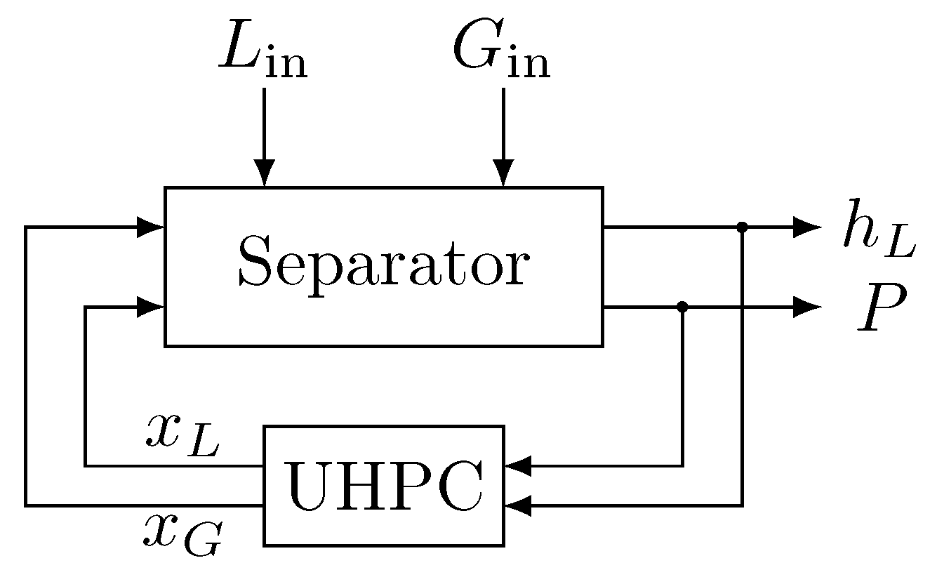
2.2.2. UHPC Design for the Biphasic Oil Separator Model

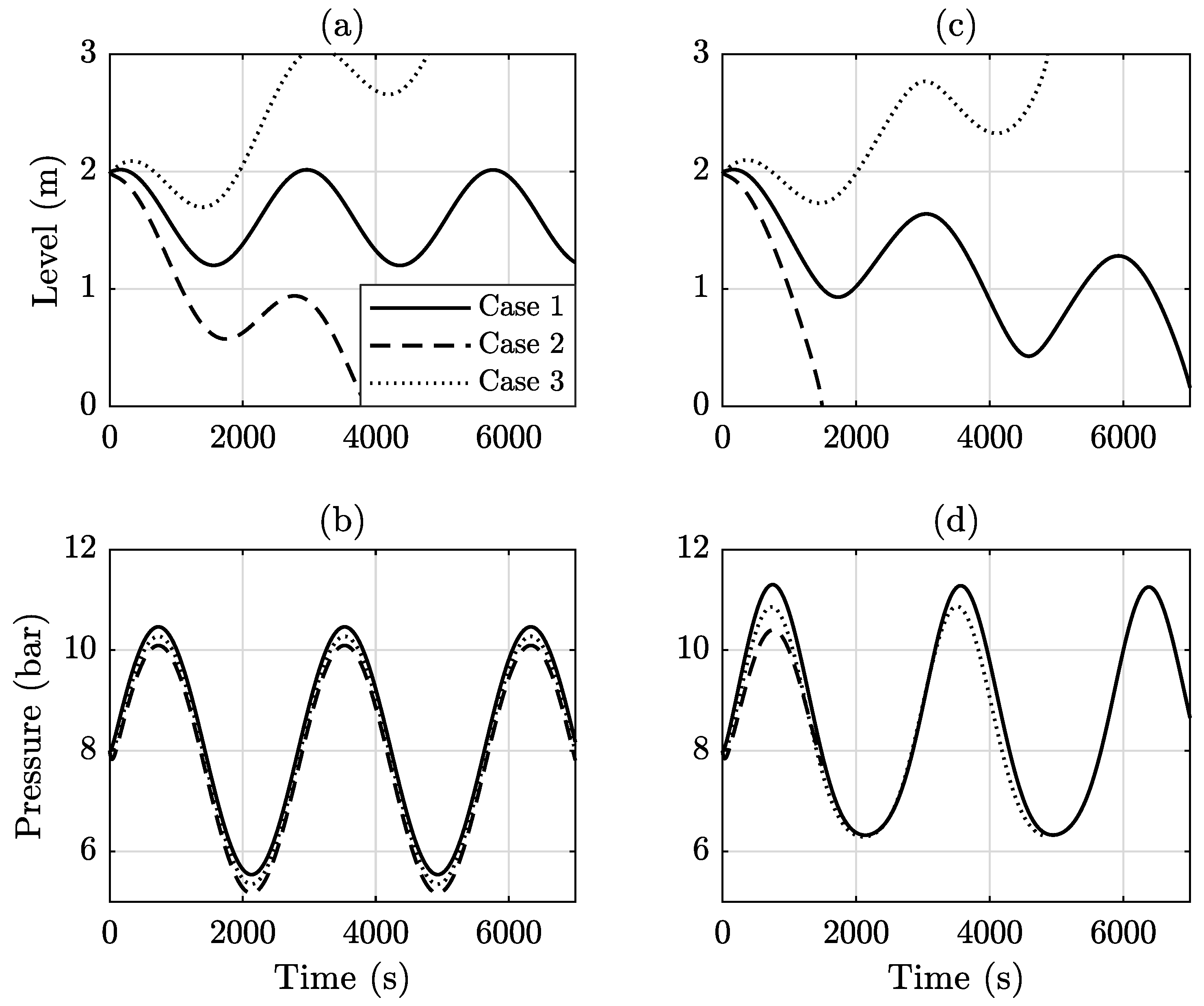
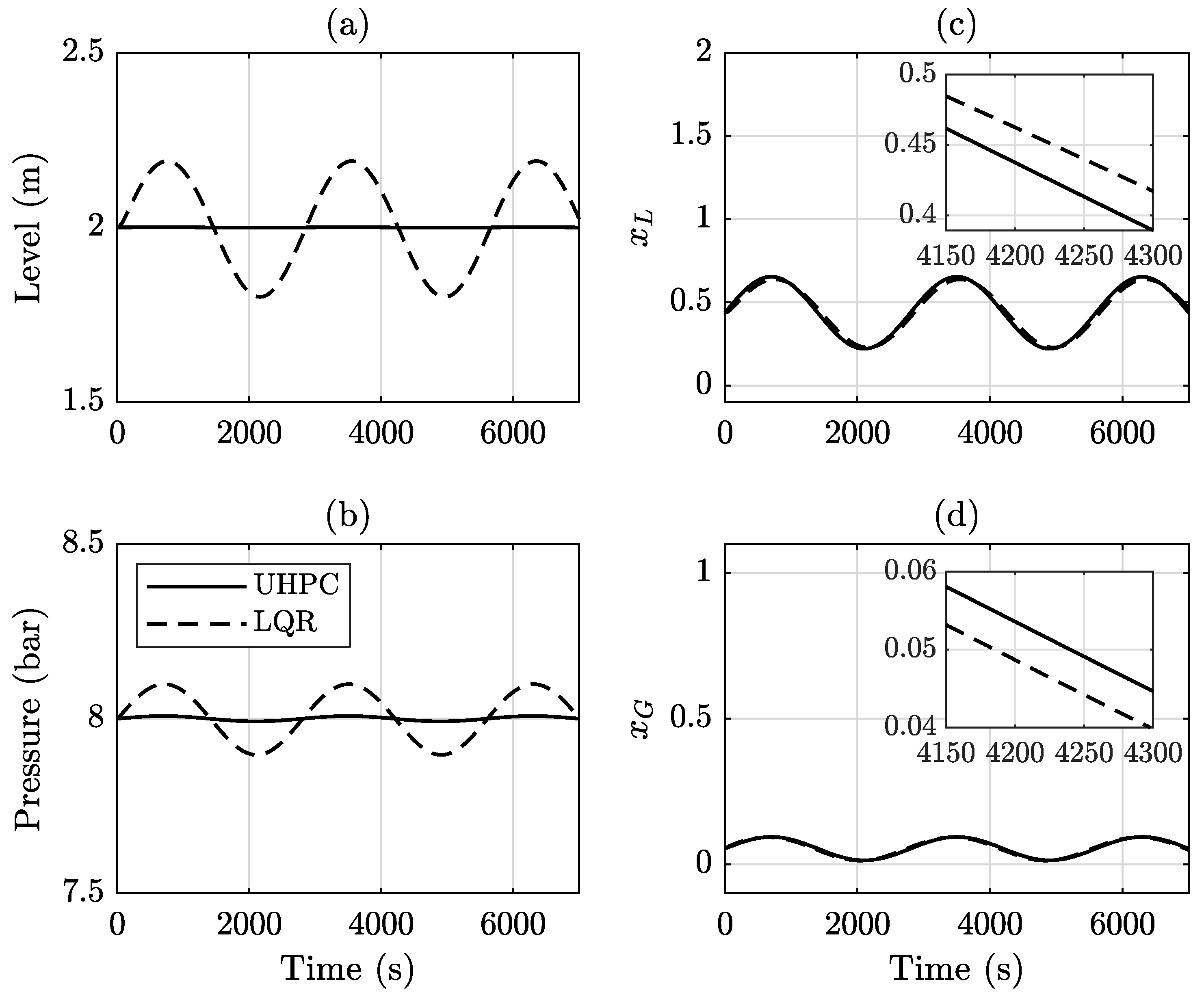
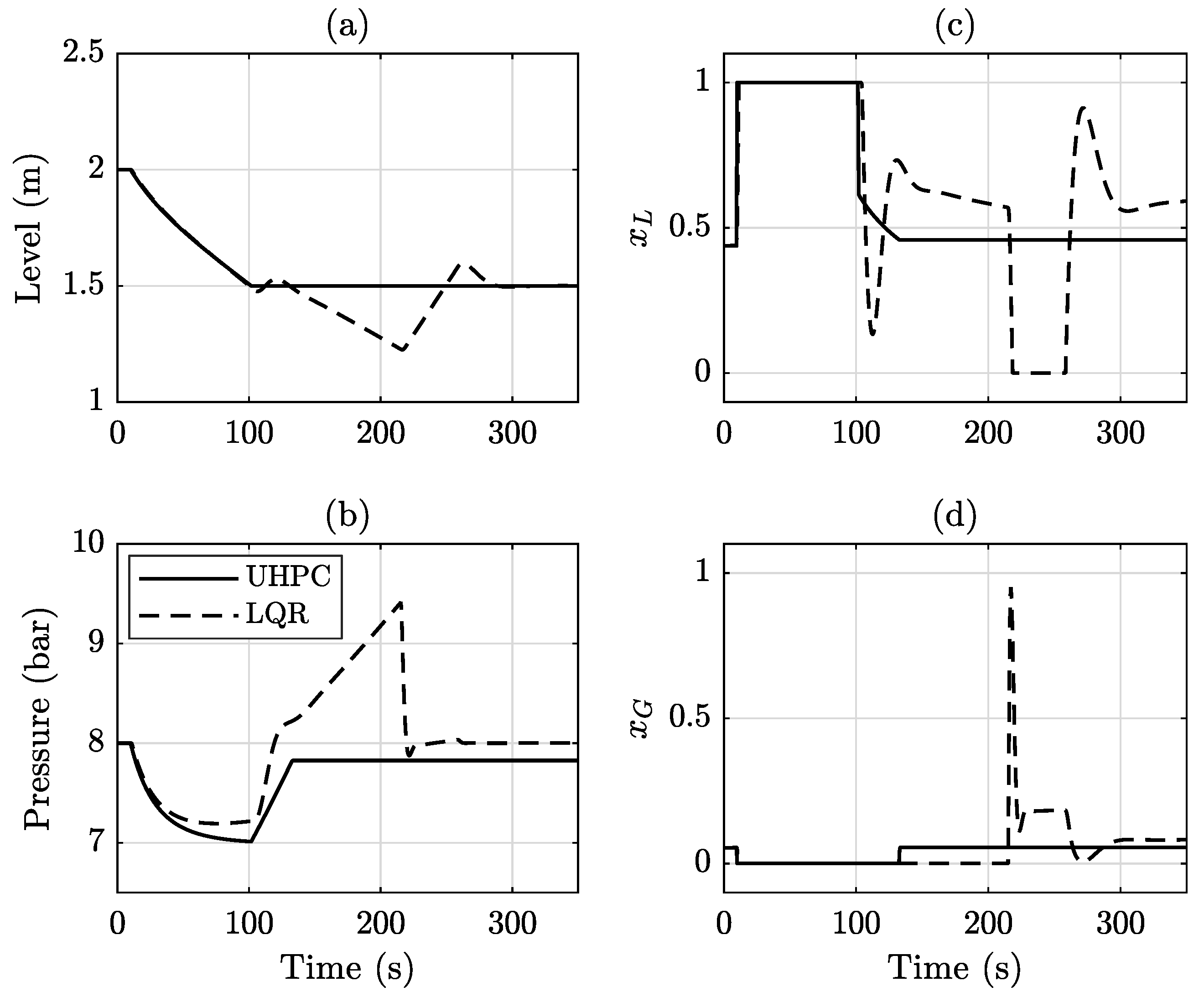
Given that the expansion of the UHPC prediction horizon $N_y$ does not burden the computational cost for its implementation, one might argue for an effective value for $N_y$. Trentini et al. [46] showed that for SISO plants, the increase in the prediction horizon makes the system’s closed-loop poles move towards its open-loop ones. Complementary to that, Trentini [47] presented the results for multivariable systems using singular value plots. It was observed that the frequency response of the closed-loop system might easily be shaped to reach the regulation prerequisites. Both cited works have shown that it is not required to increase $N_y$ further than the system’s settling time.

Hence, it is necessary to determine the biphasic oil separator’s settling time, which can be accomplished either experimentally or from its linear model. This work also regards the linearization of the separator model, given that the UHPC is a linear controller (i.e., it needs a linear model to be designed). Additionally, the reader should be aware that the separator model is approximately linear when working with small input or disturbance signals, which is exactly the case for the closed-loop system. This also allows the designer to linearise its model. This characteristic is exploited more deeply in Section 3.

Considering the nonlinear model given by Equations (1)–(7), and by applying first-order Taylor expansion, it is possible to obtain a continuous time second-order state space model with

$$\begin{array}{cc}\hfill {\mathbf{A}}_c& =\left[\begin{array}{cc}0& -0.0018\\ 0& -0.0307\end{array}\right],{\mathbf{C}}_c=\left[\begin{array}{cc}1& 0\\ 0& 1\end{array}\right],\hfill \\ \hfill {\mathbf{B}}_c& =\left[\begin{array}{cc}-0.0167& 0\\ -0.1823& -0.9019\end{array}\right],{\Gamma }_c=\left[\begin{array}{cc}0.0442& 0\\ 0.4833& 0.4833\end{array}\right],\hfill \end{array}$$

where ${\mathit{x}}_c\left(t\right)={\left[h_L\left(t\right)P\left(t\right)\right]}^T$, ${\mathit{u}}_c\left(t\right)={\left[x_L\left(t\right)x_G\left(t\right)\right]}^T$ and ${\mathbf{\xi }}_c\left(t\right)={\left[L_{\mathrm{in}}\left(t\right)G_{\mathrm{in}}\left(t\right)\right]}^T$. Both system controllability and observability are guaranteed, whilst its settling time—obtained from its eigenvalues—is 130 s. In addition, it is expected that the separator presents a natural integrator.

When considering a sampling time of $T=0.1$ s to ensure all nonlinear dynamics, the UHPC prediction horizon is $N_y=130/T=1300$ samples. It should be noted that this value is significantly higher than any previously reported in the literature, and it is possible to obtain even higher values for $N_y$ without overloading the computational capacity.

Similar to the LQR, the UHPC regards the weighting matrices $\mathbf{Q}$ and $\mathbf{R}$. The main difference is that $\mathbf{R}$ might be set to zero if one wants to use full control effort. Hence, for this work, these matrices are set to

$$\begin{array}{c}\hfill \mathbf{Q}=100·\mathbf{I},\mathbf{R}=\mathbf{0}.\end{array}$$

After system discretisation, matrices $\mathbf{F}$, $\mathbf{H}$, ${\mathbf{Y}}_0$, ${\mathbf{K}}_0$, ${\mathbf{K}}_x$, and ${\mathbf{K}}_y$ are calculated according to the description in Section 2.2. Note that $\mathbf{F}$ and $\mathbf{H}$ are the solutions of the two arisen Diophantine equations for the noise and control signal, respectively. It is also worth mentioning that there is no need for the implementation of a Kalman filter, given that both states (level and pressure) are measured. In Figure 3, the control loop is depicted. Notice the disturbance inputs $L_{\mathrm{in}}$ and $G_{\mathrm{in}}$, as well as the manipulated variables $x_L$ and $x_G$ and the measured signals $h_L$ and P.

3. Results

The biphasic oil separator nonlinear model presented in Equations (1)–(7) was implemented in MATLAB${}^{\circledR }$ and Simulink${}^{\circledR }$. All constants and steady state values displayed in Table 1 and Table 2 were considered for the simulation.

The separator’s open-loop behaviour was first simulated using $\overline{L_{\mathrm{in}}}=0.165$ m${}^3$/s and $\overline{G_{\mathrm{in}}}=0.1$ m${}^3$/s, according to Table 2. Three different fixed valves openings were used:

Case 1: 

$x_L=0.4375$ and $x_G=0.0536$ (steady state values);

Case 2: 

$x_L=0.5$ and $x_G=0.0536$ (14% increase in liquid valve opening);

Case 3: 

$x_L=0.4375$ and $x_G=0.06$ (12% increase in gas valve opening).

Figure 4 presents the obtained results with the cited values, along with the simulation of the linear plant for comparison purposes. Graphs (a) and (b) present the results for the linear plant, whilst graphs (c) and (d) show the behaviour for the nonlinear one. Notice that both models presented a pressure drop for the cases which were not the steady state case, resulting in new magnitudes after the transient (around 130 s). On the other hand, the level of liquid presented a steady increase or decrease, depending upon the valve opening. Indeed, separator linearization showed that there was a natural integrator in the system, which was expected from the modelling.

The second simulation for the open-loop system was similar to the one we just presented, but now it adds the slugs to it according to Equations (6) and (7). Figure 5 presents the obtained results. Again, graphs (a) and (b) are the level and pressure for the linear model, whilst graphs (c) and (d) are the level and pressure for the nonlinear one.

Further, simulations were conducted to compare the effectiveness of the UHPC’s control technique in regulating closed-loop behaviour for the system. The UHPC was implemented as discussed in Section 2.2, and for the sake of comparison, an LQR control scheme was also implemented. The choice for the LQR was made due to its high applicability in several multivariable processes with acknowledged success [54]. For the gravity separator shown in this paper, it was considered that $\mathbf{Q}=\mathbf{R}=100·\mathbf{I}$. According to Figure 6, which displays the results obtained from the simulation using the same slugs as in the open-loop case, both the level and pressure exhibited acceptable behaviour, with oscillations occurring at a period determined by $L_{\mathrm{in}}$ and $G_{\mathrm{in}}$ and a magnitude to the order of 10${}^{-4}$ and 10${}^{-3}$, respectively. In spite of these behaviours, the UHPC demonstrated more stable behaviour than LQR. Notice that, in Figure 6, graphs (a) and (b) are the level and pressure, respectively. Graphs (c) and (d) represent the control signals $x_L$ and $x_G$, where a zoom is included to highlight the difference between the LQR and UHPC responses.

The next simulation experimented with a change in the level reference from 2 m to 1.5 m, which is presented in Figure 7. Again, graphs (a) and (b) are the system outupts (level and pressure), whilst graphs (c) and (d) are the respective control signals $x_L$ and $x_G$. Here, the slugs were disabled to ease the analysis. The reference was changed in 10 s, where it was possible to observe abrupt changes in the valve openings. Notice that the liquid valve opened completely whilst the pressure valve closed entirely.

Lastly, a frequency response simulation was obtained for the plant (open loop) and the closed loop. Considering a multivariable (two inputs and two outputs) and nonlinear plant, the usual procedure consists of the insertion of independent sinusoidal signals with increasing frequencies (chirp) at the disturbance inputs $L_{\mathrm{in}}$ and $G_{\mathrm{in}}$ separately. Three systems were simulated: an open-loop plant and two closed-loop systems, with one utilising the UHPC and the other utilising LQR.

Figure 8 presents the obtained results for the frequency response. The upper graph (a) shows the magnitude response when $G_{\mathrm{in}}$ was kept constant at its steady state value and $L_{\mathrm{in}}$ was a chirp signal with an amplitude of 0.082 m${}^3$/s and frequency range from 0.1 mHz to 1 Hz within 28 hours of simulation. The bottom graph (b) depicts the evolution of the magnitude with an increase in frequency when $G_{\mathrm{in}}$ was regarded as a chirp signal with an amplitude of 0.075 m${}^3$/s and the same frequency and time span as in the upper graph.

4. Discussions and Conclusions

In this section, according to the obtained results, shown in Section 3, it is possible to address some discussion and highlight some paper contributions.

Considering the open-loop simulation, it can be observed in Figure 5 that both the liquid level and gas pressure presented oscillations due to the slugs. However, while the pressure just oscillated with the same period as the slugs, the level had a contrasting behaviour. Even when considering the valves’ steady state openings (solid line), the level dropped until the separator was completely empty of liquid, which occurred shortly after 7000 s. Notice that this behaviour did not occur in the linear model. Instead, it oscillated around a fixed mean level (see Figure 4a). When keeping the gas valve at its original value and opening the liquid one approximately 14% more (dashed line), it can be seen that the level of liquid reached its minimum at nearly 1500 s, which is an expected result given that more liquid was leaving the separator. On the other hand, when keeping the liquid valve at its original opening and increasing by nearly 12% the value for the gas one, the level of liquid increased inside the separator until it reached its maximum value (3 m) shortly before 5000 s. This was also expected since more gas left the system, releasing more space for the liquid. For the pressure behaviour, notice that the dashed and dash-dotted lines are displayed only until the limits for the level were reached (1500 s and 4800 s, respectively). Note also that the mean value of the pressure is not its steady state.

Some improvements were observed when the loop was closed using the proposed controller. Figure 6 shows that their oscillations were within the limits of the valves, with the means being their steady state values. We call attention to the fact that despite the highly nonlinear behaviour presented in the previous section, the dynamical behaviour of the system was nearly linear within the cited magnitude of the oscillations, with control signals $x_L$ and $x_G$ working linearly without saturation. For this reason, the usage of input constraints for the optimisation problem was not required. We remark that not considering the constraints during the optimisation procedure means that it is not possible to comply with the input limits. In this work, this fact was verified through simulations, given that constraint handling was not implemented for the UHPC yet. The determination of the input and output constraints during the optimisation procedure might be explored in works where these limits are closer to being (or are) reached.

Moreover, the control signals for the valves ($x_L$ and $x_G$) depicted in Figure 6c,d indicate that the UHPC anticipated the action over the liquid valve $x_L$ while delaying the action over the gas valve. This phenomenon occurred because making decisions based on predictions among several potential future alternatives is generally more effective than relying solely on past and present data. For instance, the UHPC can produce superior results compared with a more accurate but non-predictive LQR response.

Additionally, aiming at obtaining more information from the proposed controller effect in the outputs, a step change is required in the level set point, and the system behaviour is shown in Figure 7. As cited, the liquid valve opened completely whilst the pressure valve closed entirely. This happened due to the drop in pressure inside the separator whenever there was a negative change in the level of liquid. The level reached its new reference nearly 100 s from when the liquid valve acted again. On the other hand, the pressure of the gas started increasing as soon as the level of liquid reached the reference. This increase regards the action of the liquid valve. Note that $x_L$ reached its steady state value around 130 s, which was exactly the time when the pressure found its new stable value and the pressure valve opened again to keep it stable.

It is worth noting that the UHPC tended to produce smoother, less-oscillatory changes in both the process variables and valve control signals than LQR. This means that the UHPC can lead to more stable and predictable system behavior, while LQR may result in more abrupt and unpredictable changes.

Finally, in order to present the proposed control benefits relative to the frequency performance, the controlled plant closed-loop frequency response was obtained. Figure 8 shows that the plant had cutoff frequencies of approximately 1 mHz and 5 mHz for the liquid ($h_L$) and pressure (P) outputs, respectively. Additionally, the disturbance inputs were sharply amplified by the separator dynamics (around 50 dB in low frequencies). On the other hand, when the loop was closed using the UHPC, the system bandwidth increased to 30 mHz. This means that the closed-loop system responded 30 times faster for the liquid and 6 times faster for the pressure output, which is one of the main contributions of this paper. Moreover, it was observed that the UHPC had the potential to attenuate the impact of the low-frequency input disturbances: 3 dB for the pressure and $-18$ dB and $-78$ dB for the liquid level for input disturbances $L_{\mathrm{in}}$ and $G_{\mathrm{in}}$, respectively.

It is important to notice that LQR presented a wider bandwidth than the UHPC. On the other hand, its attenuation of external disturbances was not as effective as the UHPC.

In summary, this paper presented a novel methodology for the implementation of a model-based predictive controller in a biphasic oil separator. The unrestricted horizon predictive controller (UHPC) is shown to be an interesting option for actual implementations in the oil industry due to its simplicity, state feedback structure, and low computational effort in comparison with other members of the MPC family.

This work introduced the detailed modelling of the separator, as well as the modelling of common slug disturbances. These oscillations, which cause the accumulation of bubbles during oil extraction, are dangerous, and their impacts on the remaining platform equipment must be diminished in the gravitational separator through the action of the liquid and gas valves. Aside from that, the results for three different valve openings using the nonlinear model were presented.

It is shown that the UHPC was able to perform a fairly stable operation for the separator without overloading the prospective processor, even with the application of the modelled slug disturbances. The UHPC’s difference with other MPC models is mainly due to its intrinsic stochastic characteristic and also the implementation of its cost function. Both features together turned the UHPC into a predictive controller that uses less computer processing than the most common ones, even with the expansion of the controller’s predictive horizon until (or more than) the system’s settling time. In addition, a simulation for a 25% step-shaped decrease in the liquid level reference was explored, where it was shown that the UHPC was able to lead the level to its new operating point within less than 100 s.

Future works on this theme should include constraint calculations for the UHPC, mainly concerning its control signals. A comparison with other MPC models might also be considered. Moreover, even though the actual implementations in platforms are complex, such an implementation could also be performed in future research.

References

1. Stewart, M.; Arnold, K. Gas-Liquid and Liquid-Liquid Separators; Gulf Professional Publishing: Houston, TX, USA, 2008. [Google Scholar]
2. Bahadori, A. Natural Gas Processing; Gulf Professional Publishing: Boston, MA, USA, 2014; pp. 151–222. [Google Scholar] [CrossRef]
3. Liu, Y.; Wang, C.; Cai, J.; Lu, H.; Huang, L.; Yang, Q. Pilot application of a novel Gas–Liquid separator on offshore platforms. J. Pet. Sci. Eng. 2019, 180, 240–245. [Google Scholar] [CrossRef]
4. Constant-Machado, H.; Leclerc, J.P.; Avilan, E.; Landaeta, G.; Añorga, N.; Capote, O. Flow modeling of a battery of industrial crude oil/gas separators using 113mIn tracer experiments. Chem. Eng. Process. Process Intensif. 2005, 44, 760–765. [Google Scholar] [CrossRef]
5. Acharya, T.; Casimiro, L. Evaluation of flow characteristics in an onshore horizontal separator using computational fluid dynamics. J. Ocean. Eng. Sci. 2020, 5, 261–268. [Google Scholar] [CrossRef]
6. Ayala, H.L.F.; Alp, D.; Al-Timimy, M. Intelligent design and selection of natural gas two-phase separators. J. Nat. Gas Sci. Eng. 2009, 1, 84–94. [Google Scholar] [CrossRef]
7. Mostafaiyan, M.; Saeb, M.R.; Alorizi, A.E.; Farahani, M. Application of evolutionary computational approach in design of horizontal three-phase gravity separators. J. Pet. Sci. Eng. 2014, 119, 28–35. [Google Scholar] [CrossRef]
8. Grødal, E.O.; Realff, M.J. Optimal design of two-and three-phase separators: A mathematical programming formulation. In Proceedings of the SPE Annual Technical Conference and Exhibition, Society of Petroleum Engineers, Huston, TX, USA, 3–6 October 1999. [Google Scholar]
9. Song, J.; Hu, X.; Zhang, J.; Chen, J. Experimental study on performance of two types of corrugated plate gas-liquid separators. Energy Procedia 2017, 142, 3282–3286. [Google Scholar] [CrossRef]
10. Skjefstad, H.S.; Stanko, M. Experimental performance evaluation and design optimization of a horizontal multi-pipe separator for subsea oil-water bulk separation. J. Pet. Sci. Eng. 2019, 176, 203–219. [Google Scholar] [CrossRef]
11. Hreiz, R. On the effect of the nozzle design on the performances of gas–liquid cylindrical cyclone separators. Int. J. Multiph. Flow 2014, 58, 15–26. [Google Scholar] [CrossRef]
12. Ahmed, T.; Russell, P.A.; Makwashi, N.; Hamad, F.; Gooneratne, S. Design and capital cost optimisation of three-phase gravity separators. Heliyon 2020, 6, e04065. [Google Scholar] [CrossRef]
13. Pedersen, S.; Durdevic, P.; Yang, Z. Challenges in slug modeling and control for offshore oil and gas productions: A review study. Int. J. Multiph. Flow 2017, 88, 270–284. [Google Scholar] [CrossRef]
14. Sausen, A.; Sausen, P.; Campos, M. Chapter 5—The Slug Flow Problem in Oil Industry and Pi Level Control. In New Technologies in the Oil and Gas Industry; Gomes, J.S., Ed.; IntechOpen: London, UK, 2012; pp. 103–116. [Google Scholar] [CrossRef]
15. Cozin, C.; Vicencio, F.E.C.; de Almeida Barbuto, F.A.; Morales, R.E.M.; da Silva, M.J.; Arruda, L.V.R. Two-Phase Slug Flow Characterization Using Artificial Neural Networks. IEEE Trans. Instrum. Meas. 2016, 65, 494–501. [Google Scholar] [CrossRef]
16. Dong, X.; Tan, C.; Dong, F. Gas–Liquid Two-Phase Flow Velocity Measurement With Continuous Wave Ultrasonic Doppler and Conductance Sensor. IEEE Trans. Instrum. Meas. 2017, 66, 3064–3076. [Google Scholar] [CrossRef]
17. Zhao, Z.; Shi, B. Numerical simulation of oil-water separation process in disc separator. In Proceedings of the 2011 International Conference on Remote Sensing, Environment and Transportation Engineering, Nanjing, China, 24–26 June 2011; pp. 8369–8372. [Google Scholar] [CrossRef]
18. Nemoto, R.H.; Baliño, J.L. Modeling and simulation of severe slugging with mass transfer effects. Int. J. Multiph. Flow 2012, 40, 144–157. [Google Scholar] [CrossRef]
19. Backi, C.J.; Krishnamoorthy, D.; Skogestad, S. Slug handling with a virtual harp based on nonlinear predictive control for a gravity separator. IFAC-PapersOnLine 2018, 51, 120–125. [Google Scholar] [CrossRef]
20. Hernandez-Perez, V.; Abdulkadir, M.; Azzopardi, B.J. Slugging Frequency Correlation for Inclined Gas-liquid Flow. Int. J. Chem. Mol. Eng. 2010, 4, 10–17. [Google Scholar]
21. Liu, W.; Han, Y.; Wang, D.; Zhao, A.; Jin, N. The Slug and Churn Turbulence Characteristics of Oil–Gas–Water Flows in a Vertical Small Pipe. Z. FüR Naturforschung 2017, 72, 817–831. [Google Scholar] [CrossRef]
22. Godhavn, J.M.; Fard, M.P.; Fuchs, P.H. New slug control strategies, tuning rules and experimental results. J. Process Control 2005, 15, 547–557. [Google Scholar] [CrossRef]
23. Mokhatab, S.; Poe, W.A.; Mak, J.Y. Handbook of Natural Gas Transmission and Processing, 4th ed.; Gulf Professional Publishing: Huston, TX, USA, 2019; pp. 103–176. [Google Scholar] [CrossRef]
24. Havre, K.; Dalsmo, M. Active Feedback Control as a Solution to Severe Slugging. Spe Prod. Facil. 2002, 17, 138–148. [Google Scholar] [CrossRef] [Green Version]
25. Pinto, D.D.D.; Araújo, O.Q.; de Medeiros, J.L.; Nunes, G.C. Slug Control Structures for Mitigation of Disturbances to Offshore Units. In 10th International Symposium on Process Systems Engineering: Part A; Elsevier: Amsterdam, The Netherlands, 2009; Volume 27, pp. 1305–1310. [Google Scholar] [CrossRef]
26. Nunes, G.C.; Coelho, A.A.R.; Sumar, R.R.; Mejía, R.I.G. Band Control: Concepts and Application in Dampening oscillations of Feed of Petroleum Production Units. IFAC Proc. Vol. 2005, 38, 123–128. [Google Scholar] [CrossRef] [Green Version]
27. Nunes, G.C. Design and Analysis of Multivariable Predictive Control Applied to an Oil-Water-Gas Separator: A Polynomial Approach; University of Florida: Gainesville, FL, USA, 2001. [Google Scholar]
28. Minghui, W.; Gensheng, L. Wellbore Temperature Prediction and Control Through State Space Model. In Proceedings of the SPE Kingdom of Saudi Arabia Annual Technical Symposium and Exhibition, OnePetro, Dammam, Saudi Arabia, 25–28 April 2016. [Google Scholar]
29. Liu, X.; Liu, Z.; Wang, X.; Zhang, N.; Qiu, N.; Chang, Y.; Chen, G. Recoil control of deepwater drilling riser system based on optimal control theory. Ocean. Eng. 2021, 220, 108473. [Google Scholar] [CrossRef]
30. Veremey, E.I. Optimal damping stabilisation based on LQR synthesis. Int. J. Syst. Sci. 2020, 52, 1359–1372. [Google Scholar] [CrossRef]
31. Shim, K.H.; Sawan, M.E. Linear quadratic regulator design for singularly perturbed systems by unified approach using d operators. Int. J. Syst. Sci. 2001, 32, 1119–1125. [Google Scholar] [CrossRef]
32. Lincoln, B.; Bernhardsson, B. LQR optimization of linear system switching. IEEE Trans. Autom. Control 2002, 47, 1701–1705. [Google Scholar] [CrossRef]
33. Patarroyo-Montenegro, J.F.; Andrade, F.; Guerrero, J.M.; Vasquez, J.C. A Linear Quadratic Regulator With Optimal Reference Tracking for Three-Phase Inverter-Based Islanded Microgrids. IEEE Trans. Power Electron. 2021, 36, 7112. [Google Scholar] [CrossRef]
34. Rossiter, J.A. Model-Based Predictive Control: A Practical Approach; CRC Press: Boca Raton, FL, USA, 2017. [Google Scholar]
35. Stokke, S.; Strand, S.; Sjong, D. Model predictive control (MPC) of a gas-oil-water separator train. In Methods of Model Based Process Control; Springer: Berlin/Heidelberg, Germany, 1995; pp. 701–713. [Google Scholar]
36. Mendes, P.; Normey-Rico, J.E.; Plucenio, A.; Carvalho, R. Disturbance estimator based nonlinear MPC of a three phase separator. IFAC Proc. Vol. 2012, 45, 101–106. [Google Scholar] [CrossRef] [Green Version]
37. Hansen, L.; Durdevic, P.; Jepsen, K.L.; Yang, Z. Plant-wide optimal control of an offshore de-oiling process using mpc technique. IFAC-PapersOnLine 2018, 51, 144–150. [Google Scholar] [CrossRef]
38. Jespersen, S.; Yang, Z. Performance Evaluation of a De-oiling Process Controlled by PID, H and MPC. In Proceedings of the IECON 2021—47th Annual Conference of the IEEE Industrial Electronics Society, Toronto, ON, Canada, 13–16 October 2021. [Google Scholar]
39. Bitmead, R.R.; Gevers, M.; Wertz, V. Adaptive Optimal Control—The Thinking Man’s GPC; Prentice Hall: Hoboken, NJ, USA, 1990. [Google Scholar]
40. Clarke, D.; Mohtadi, C.; Tuffs, P. Generalized predictive controller—Part I: The basic algorithm. Automatica 1987, 23, 137–148. [Google Scholar] [CrossRef]
41. Ribeiro, C.; Miyoshi, S.; Secchi, A.; Bhaya, A. Model Predictive Control with quality requirements on petroleum production platforms. J. Pet. Sci. Eng. 2016, 137, 10–21. [Google Scholar] [CrossRef]
42. Neto, S.S.; Secchi, A. Nonlinear Model Predictive Controller Applied to an Offshore Oil and Gas Production Facility. In Proceedings of the OTC Brasil, OnePetro, Rio de Janeiro, Brasil, 24–26 October 2017. [Google Scholar]
43. Campos, M.C.M.M.; Ribeiro, L.D.; Diehl, F.C.; Moreira, C.A.; Bombardelli, D.; Carelli, A.C.; Junior, G.M.J.; Pinto, S.F.; Quaresma, B. Intelligent System for Start-Up and Anti-Slug Control of a Petroleum Offshore Platform. In Proceedings of the Offshore Technology Conference, Houston, TX, USA, 1–4 May 2017. [Google Scholar] [CrossRef]
44. Willersrud, A.; Imsland, L.; Hauger, S.O.; Kittilsen, P. Short-term production optimization of offshore oil and gas production using nonlinear model predictive control. J. Process Control 2013, 23, 215–223. [Google Scholar] [CrossRef] [Green Version]
45. Richalet, J.; Rault, A.; Testud, J.; Papon, J. Model predictive heuristic control: Applications to industrial processes. Automatica 1978, 14, 413–428. [Google Scholar] [CrossRef]
46. Trentini, R.; Silveira, A.; Kutzner, R.; Hofmann, L. On the unrestricted horizon predictive control—A fully stochastic model-based predictive approach. In Proceedings of the 2016 European Control Conference (ECC) IEEE, Aalborg, Denmark, 29 June–1 July 2016; pp. 1322–1327. [Google Scholar]
47. Trentini, R. Contributions to the Damping of Interarea Modes in Extended Power Systems: A Turbine Governor Approach with the Help of the Unrestricted Horizon Predictive Controller. Ph.D. Thesis, Gottfried Wilhelm Leibniz Universität, Hannover, Germany, 2017. [Google Scholar]
48. De Lima, J.C., Jr.; Trentini, R.; Prioste, F. Comparative study of the pitch control of a wind turbine using Linear Quadratic Gaussian and the Unrestricted Horizon Predictive Controller. Int. Trans. Electr. Energy Syst. 2021, 31, e12720. [Google Scholar]
49. De Castro, L.A.; Silveira, A.d.S.; Araújo, R.d.B. Unrestricted horizon predictive control applied to a nonlinear SISO system. Int. J. Dyn. Control 2022, 11, 286–300. [Google Scholar] [CrossRef]
50. Yan, K.; Che, D. Hydrodynamic and mass transfer characteristics of slug flow in a vertical pipe with and without dispersed small bubbles. Int. J. Multiph. Flow 2011, 37, 299–325. [Google Scholar] [CrossRef]
51. Nunes, G.C.; de Medeiros, J.L.; Araújo, O.; de Queiroz Fernandes, O. Modelagem e Controle da Produçao de Petróleo: Aplicaçoes em Matlab; Editora Blucher: São Paulo, Brazil, 2010. [Google Scholar]
52. Perry, R.H.; Green, D.W. Perry’s Chemical Engineer’s Handbook, 6th ed.; McGraw-Hill Book Co.: New York, NY, USA, 1985. [Google Scholar]
53. Silveira, A.S.; Coelho, A.A. Generalised minimum variance control state-space design. IET Control Theory Appl. 2011, 5, 1709–1715. [Google Scholar] [CrossRef]
54. Berkovitz, L.D. Optimal Control Theory; Springer Science & Business Media: Berlin/Heidelberg, Germany, 2013; Volume 12. [Google Scholar]
Figure 1. Schematic of a slug flow [50].
Processes 11 00928 g001
Figure 2. Biphasic gravitational separator.
Processes 11 00928 g002
Figure 3. Control loop for the oil separator with UHPC.
Processes 11 00928 g003
Figure 4. Simulation of the linear and nonlinear plants for different valve openings. (a,b) the results for the linear plant; (c,d) the behaviour for the nonlinear one.
Processes 11 00928 g004
Figure 5. Simulation of the linear and nonlinear plants for different valve openings with slugs. (a,b) the level and pressure for the linear model; (c,d) the level and pressure for the nonlinear one.
Processes 11 00928 g005
Figure 6. Simulation of the closed-loop system with slug disturbance. (a,b) the level and pressure, respectively; (c,d) the control signals x L and x G , where a zoom is included to highlight the difference between the LQR and UHPC responses.
Processes 11 00928 g006
Figure 7. Simulation of the closed-loop system for step decrease in level reference. (a,b) the system outupts (level and pressure); (c,d) the respective control signals x L and x G .
Processes 11 00928 g007
Figure 8. Frequency response of open- and closed-loop systems (a) with L in as input and (b) with G in as input.
Processes 11 00928 g008